
Assessment of Hydrological Processes in an Ungauged Catchment in Eritrea


Abstract
:1. Introduction
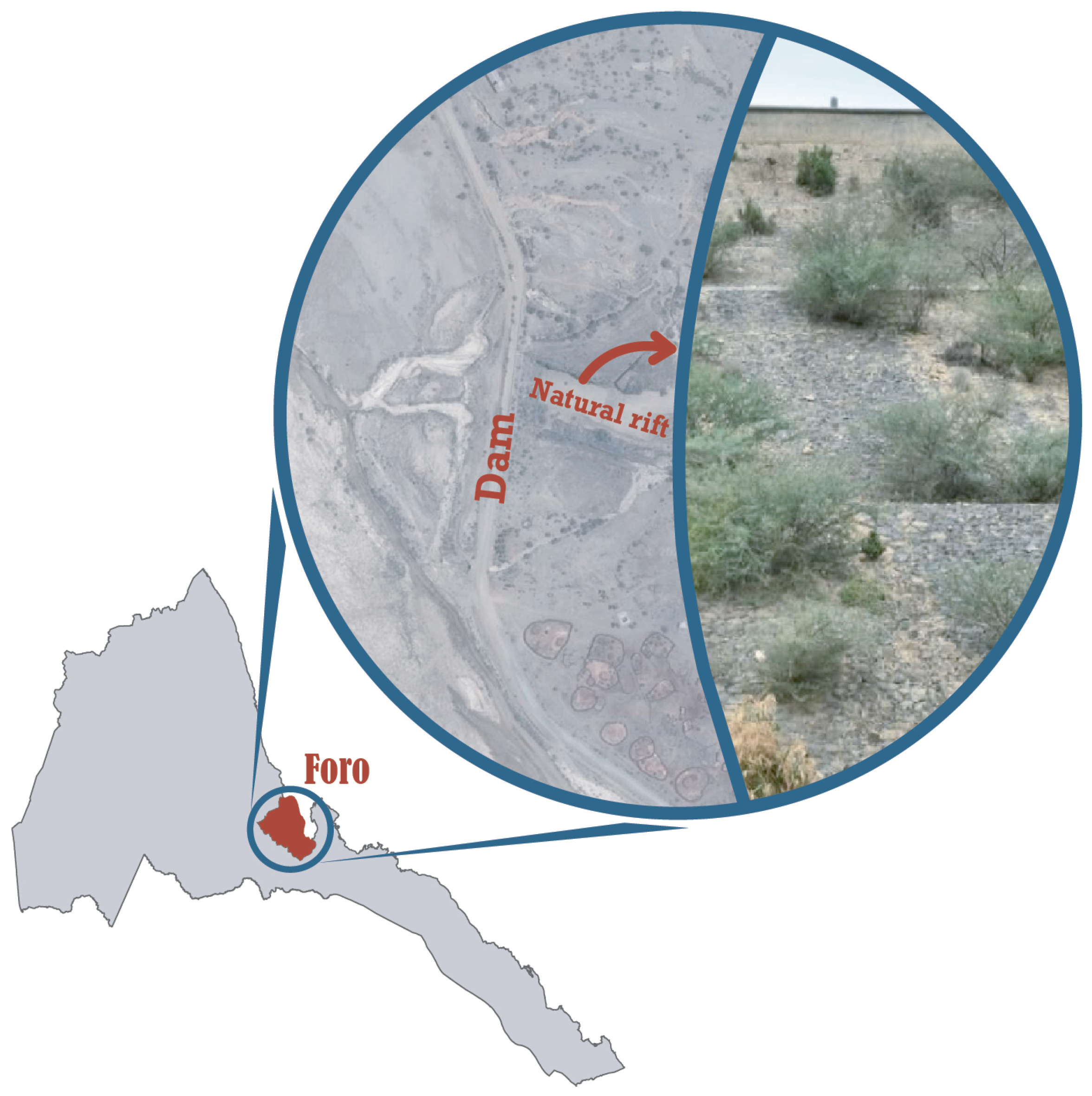
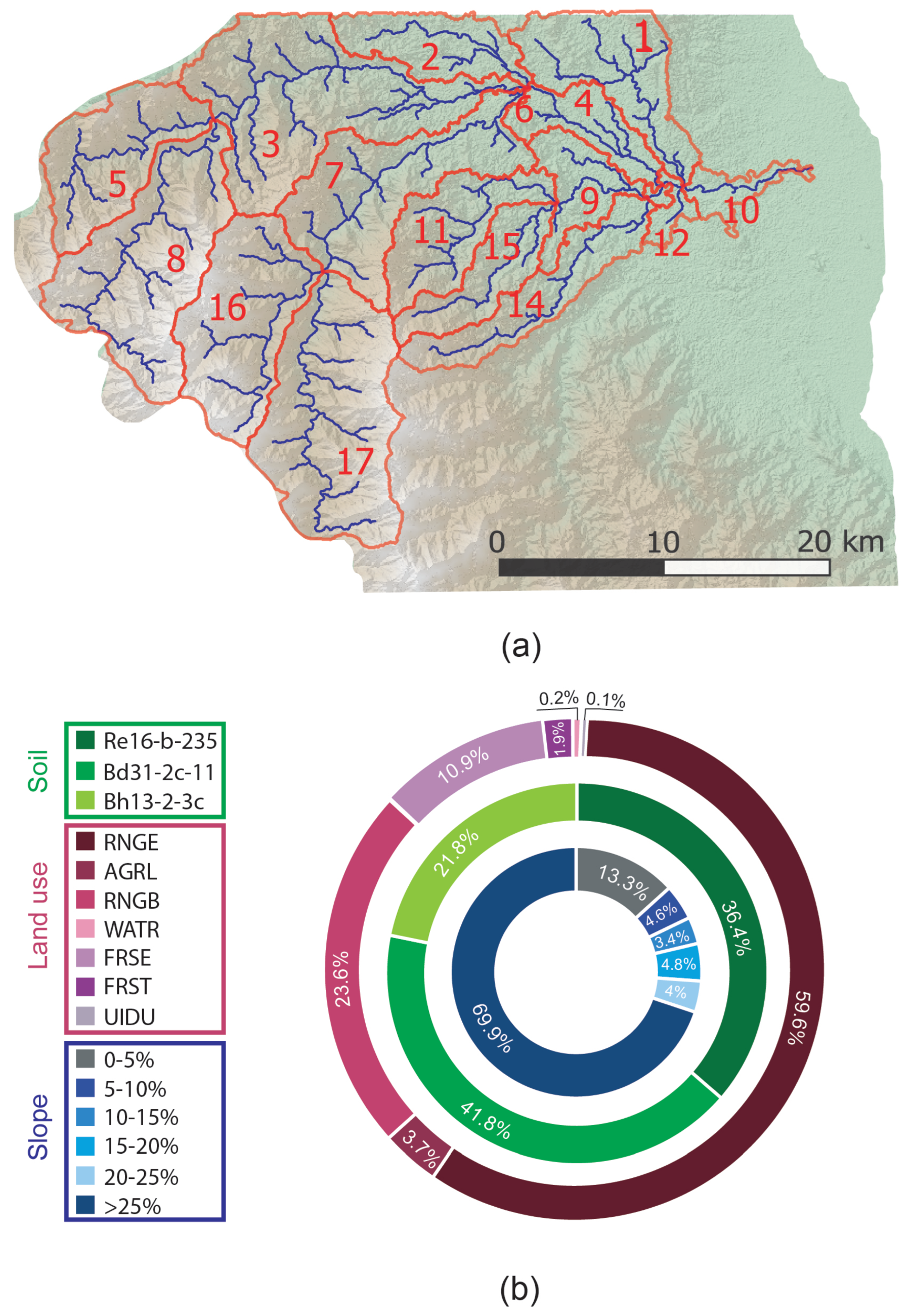
2. Study Site
3. Data Collection
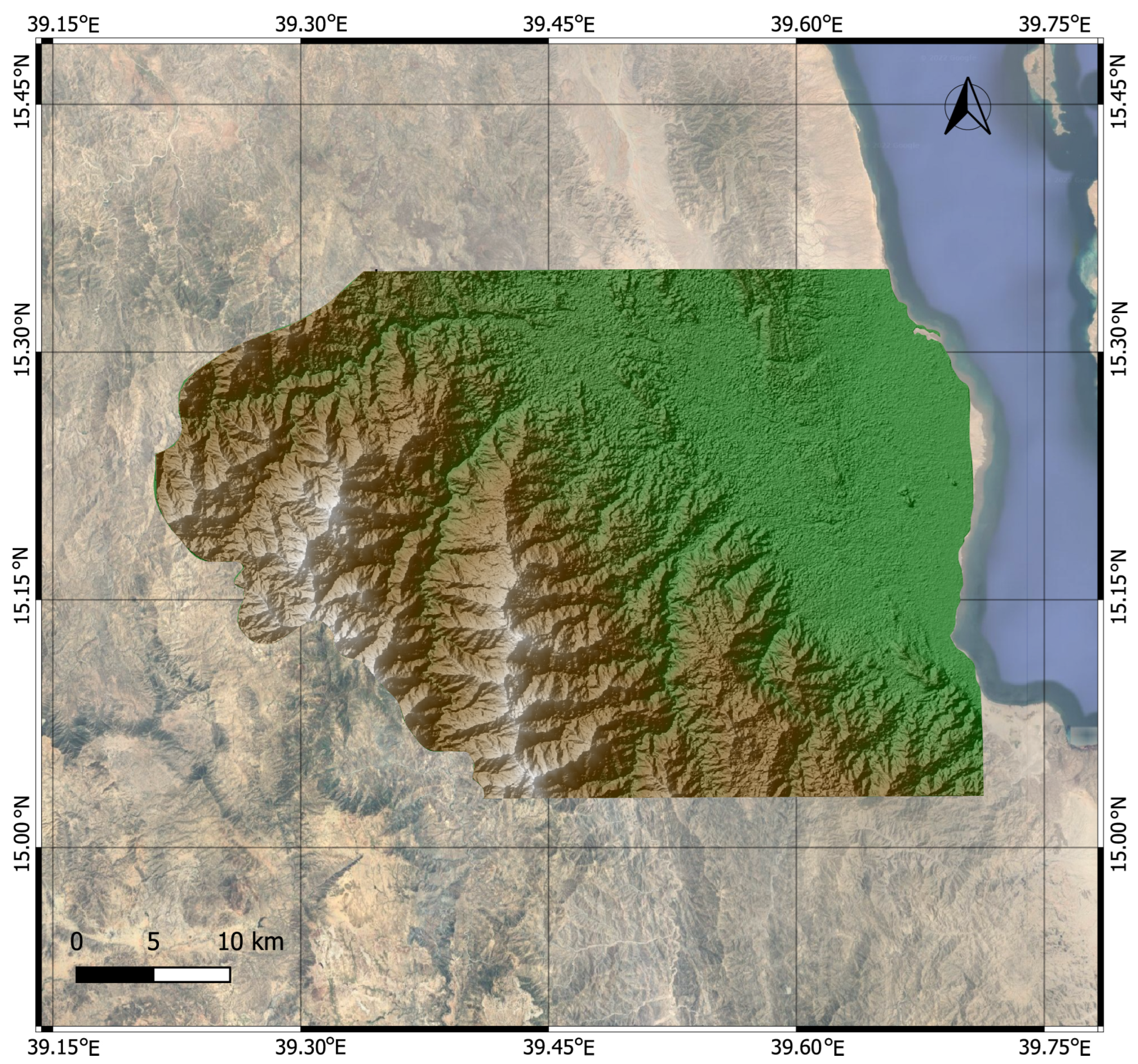
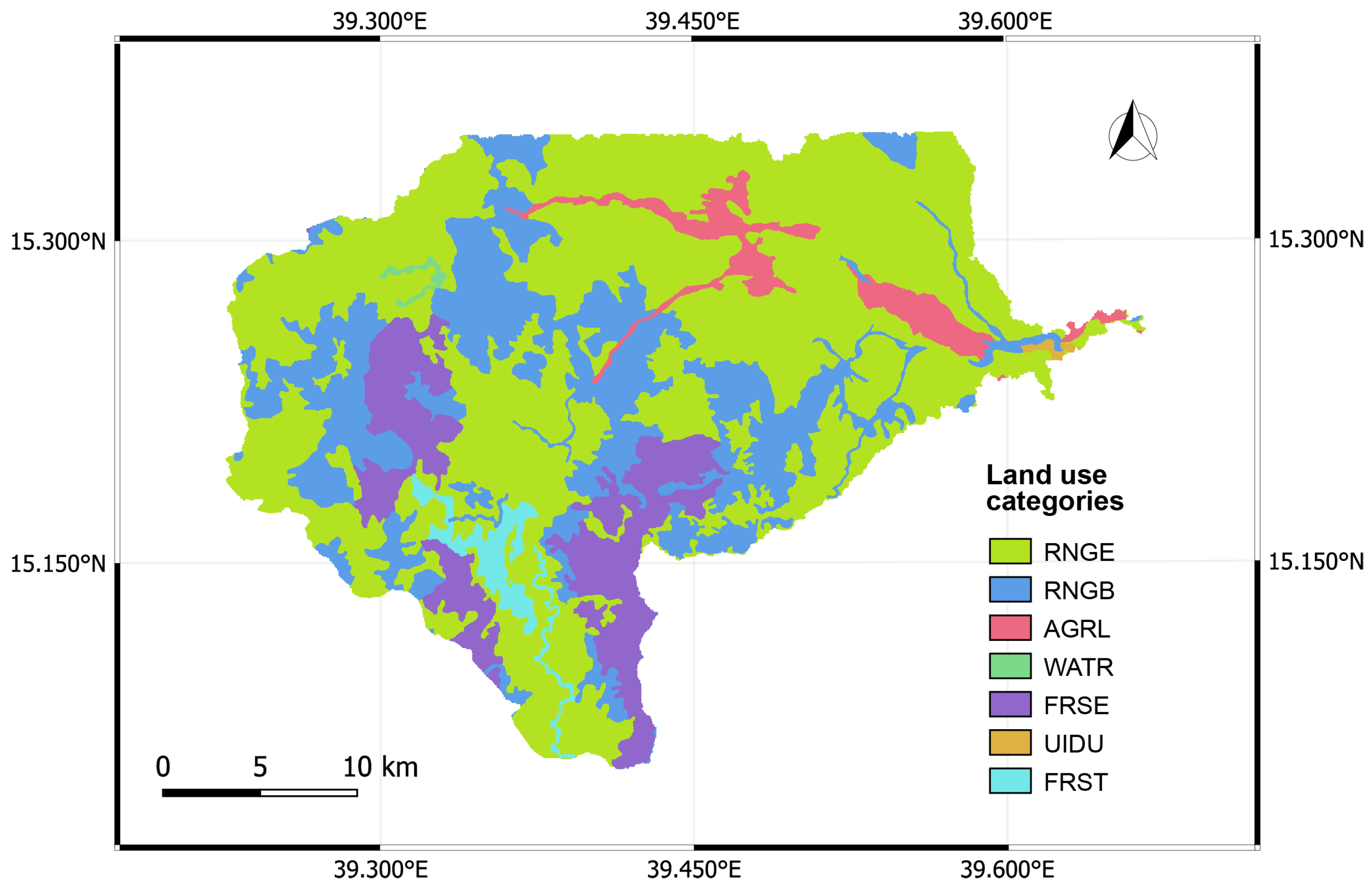
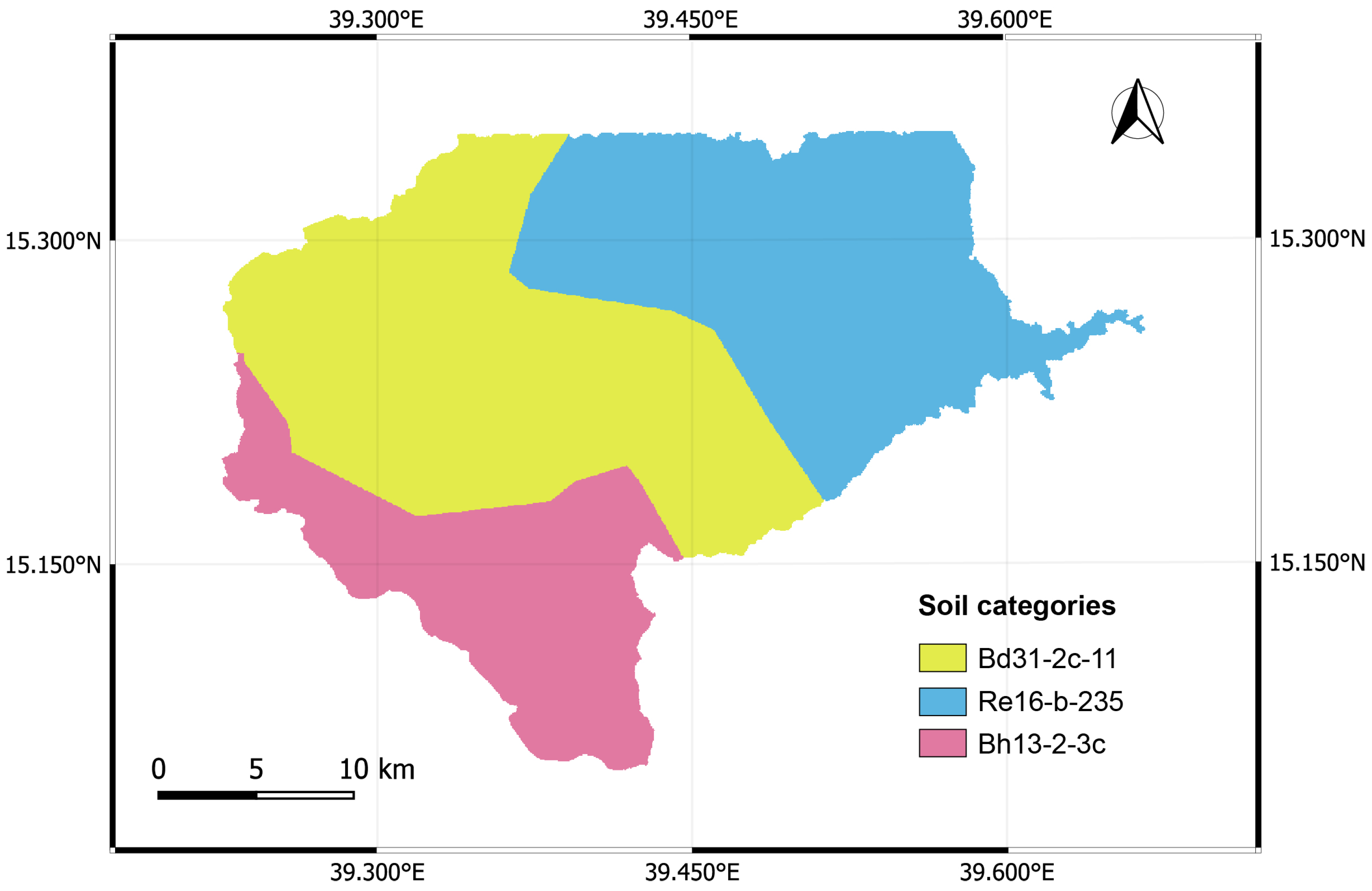
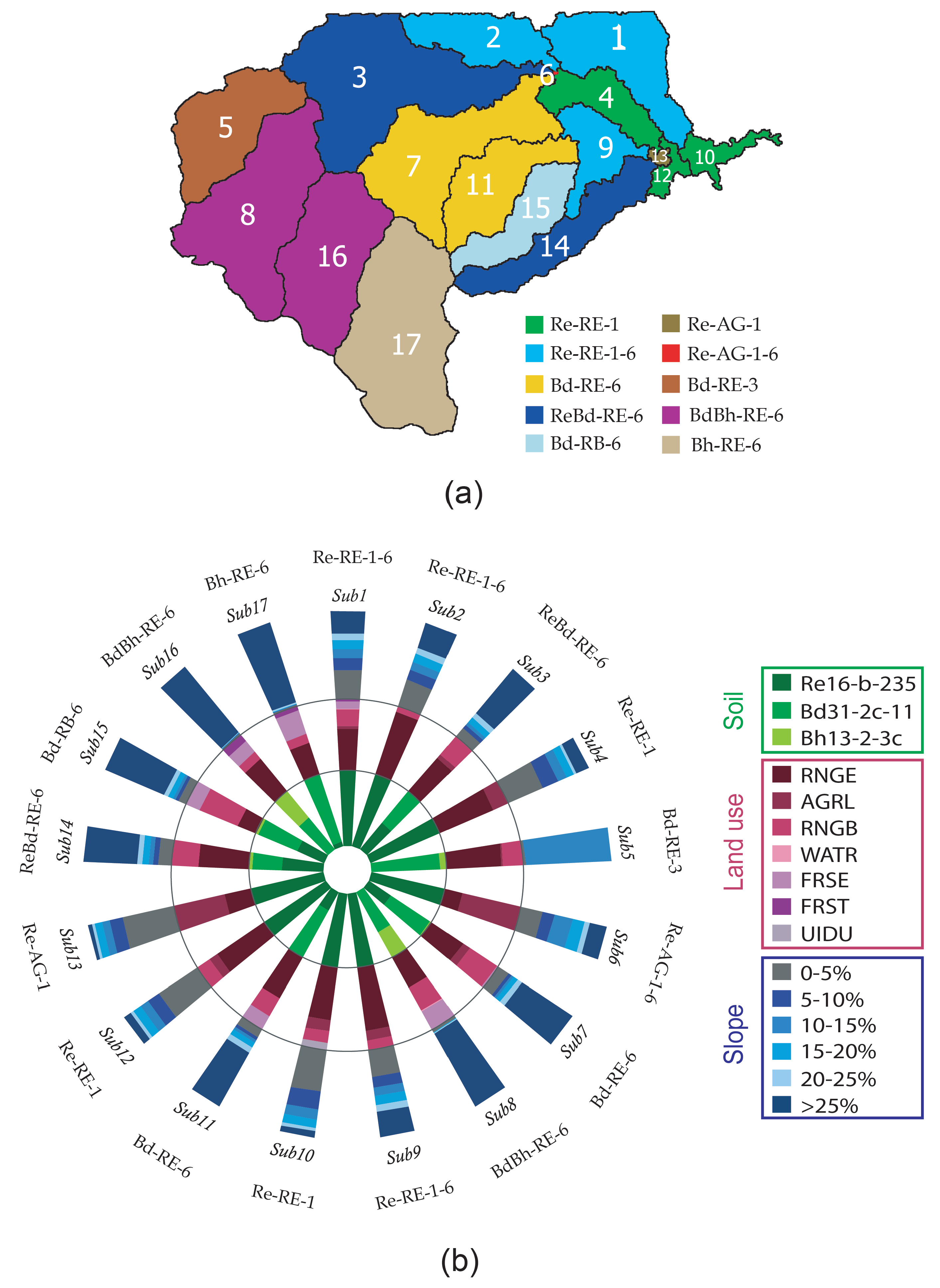
3.1. Digital Elevation Model, Land Cover, and Soil Properties
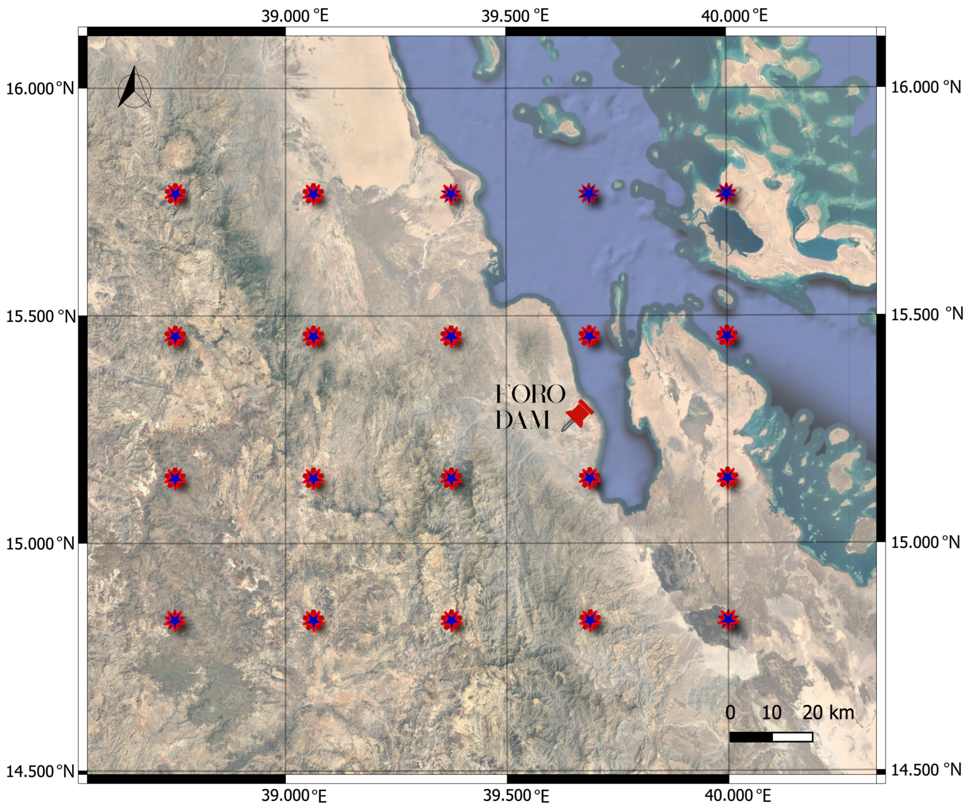
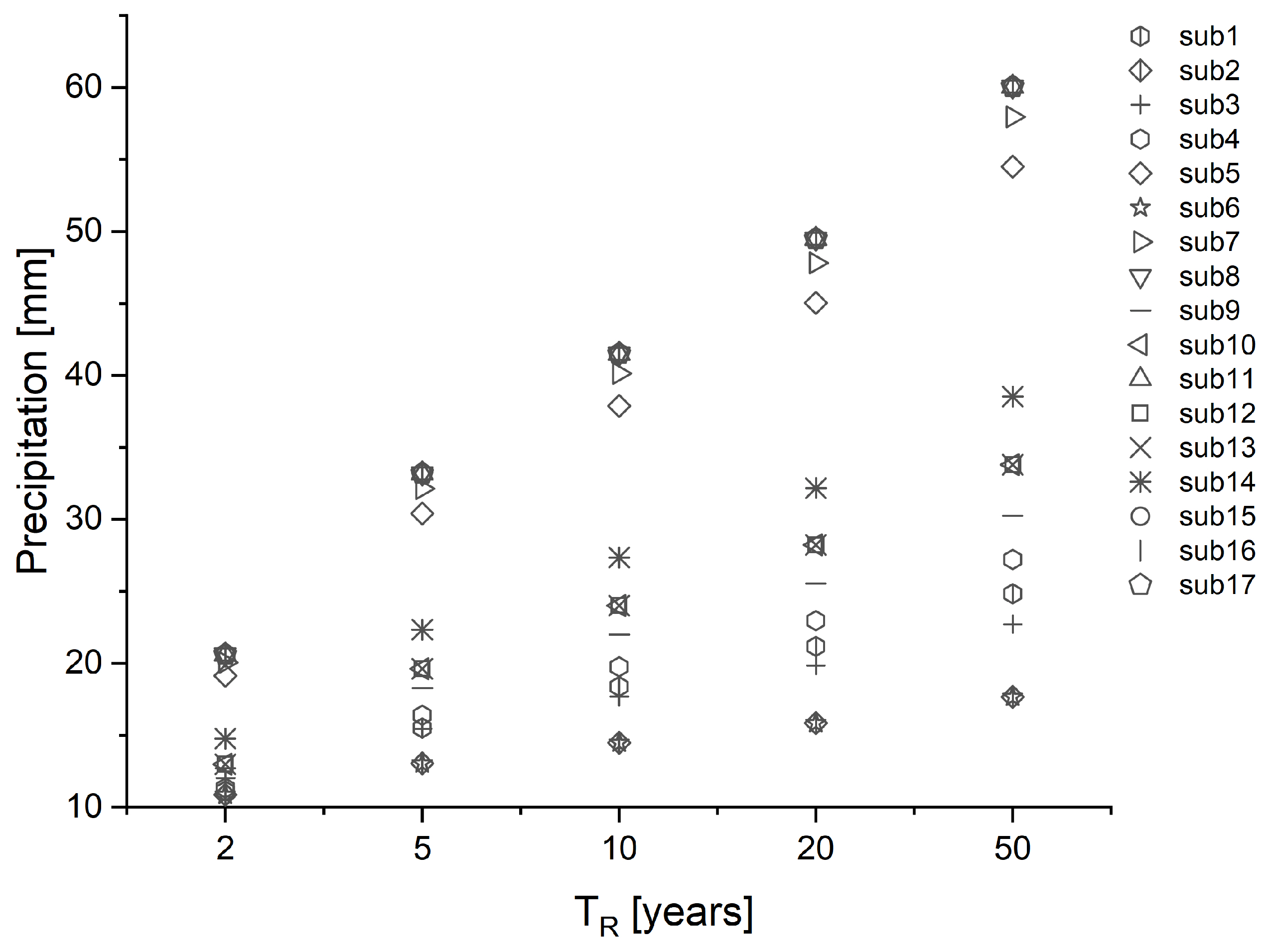
3.2. Climatic Data
4. Preprocessing Analysis
5. Hydrological Model
5.1. Surface Processes: Runoff and Evapotranspiration
5.2. Subsurface Water Balance
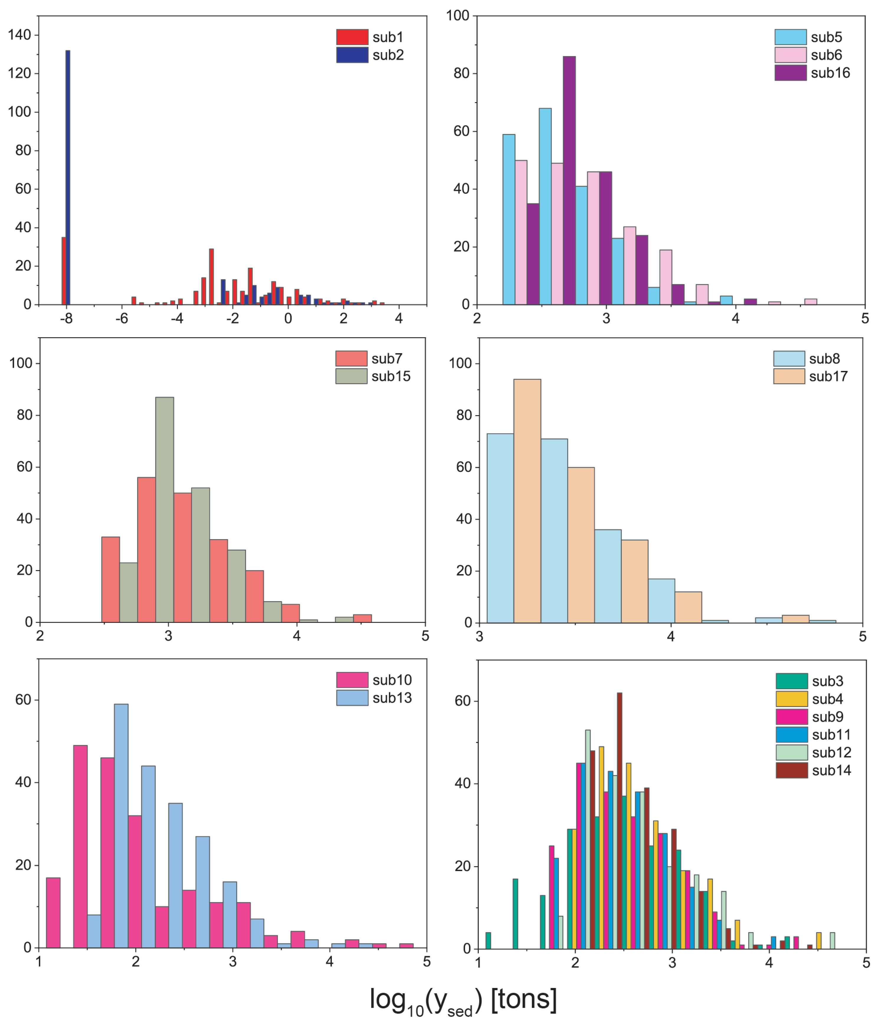
5.3. Erosion
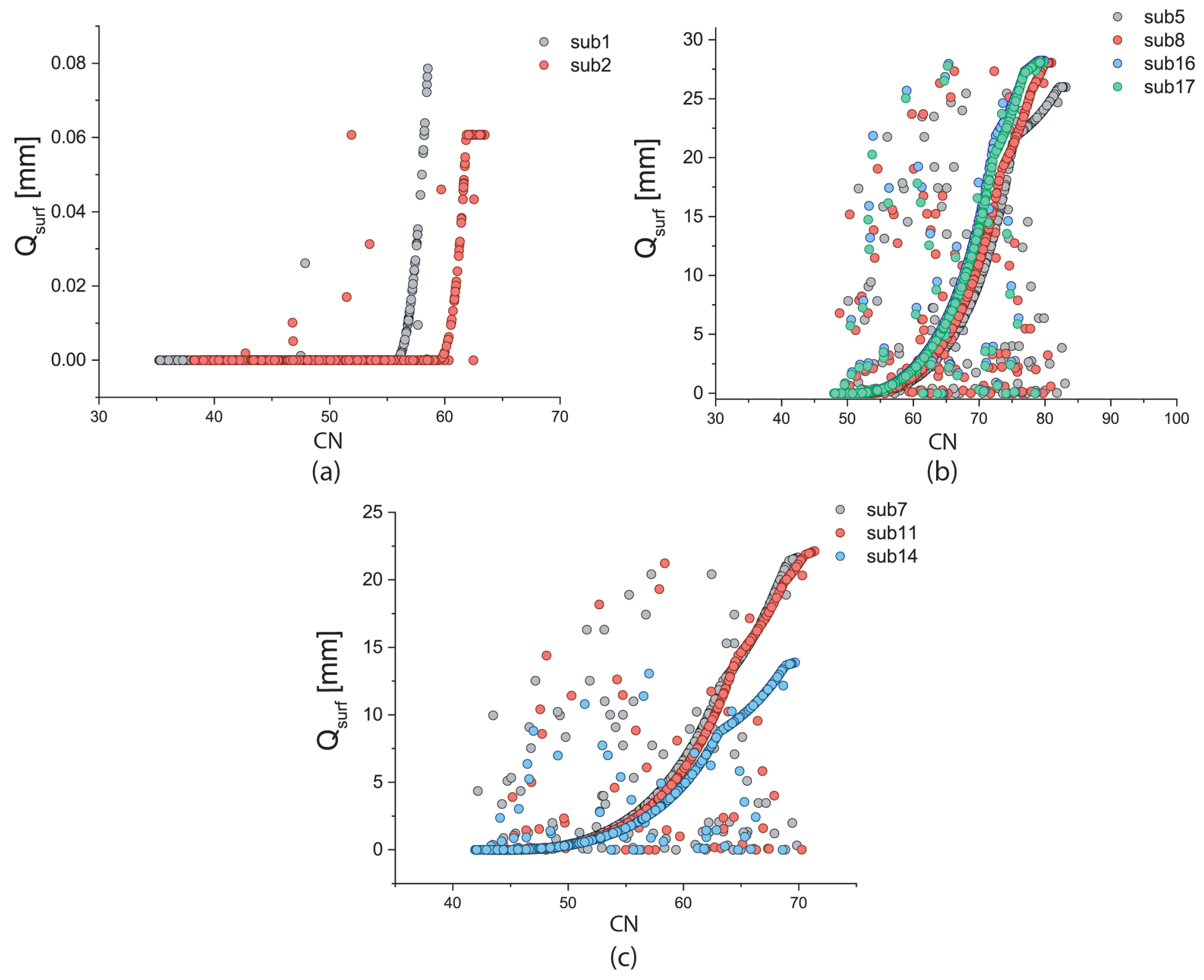
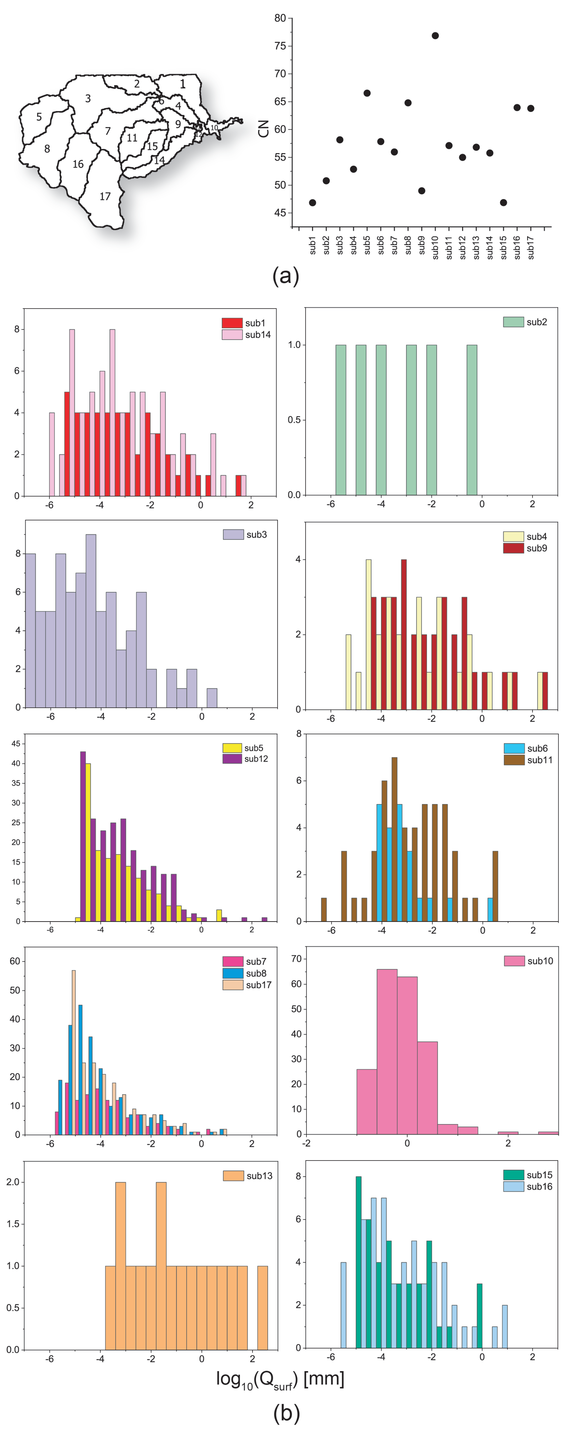
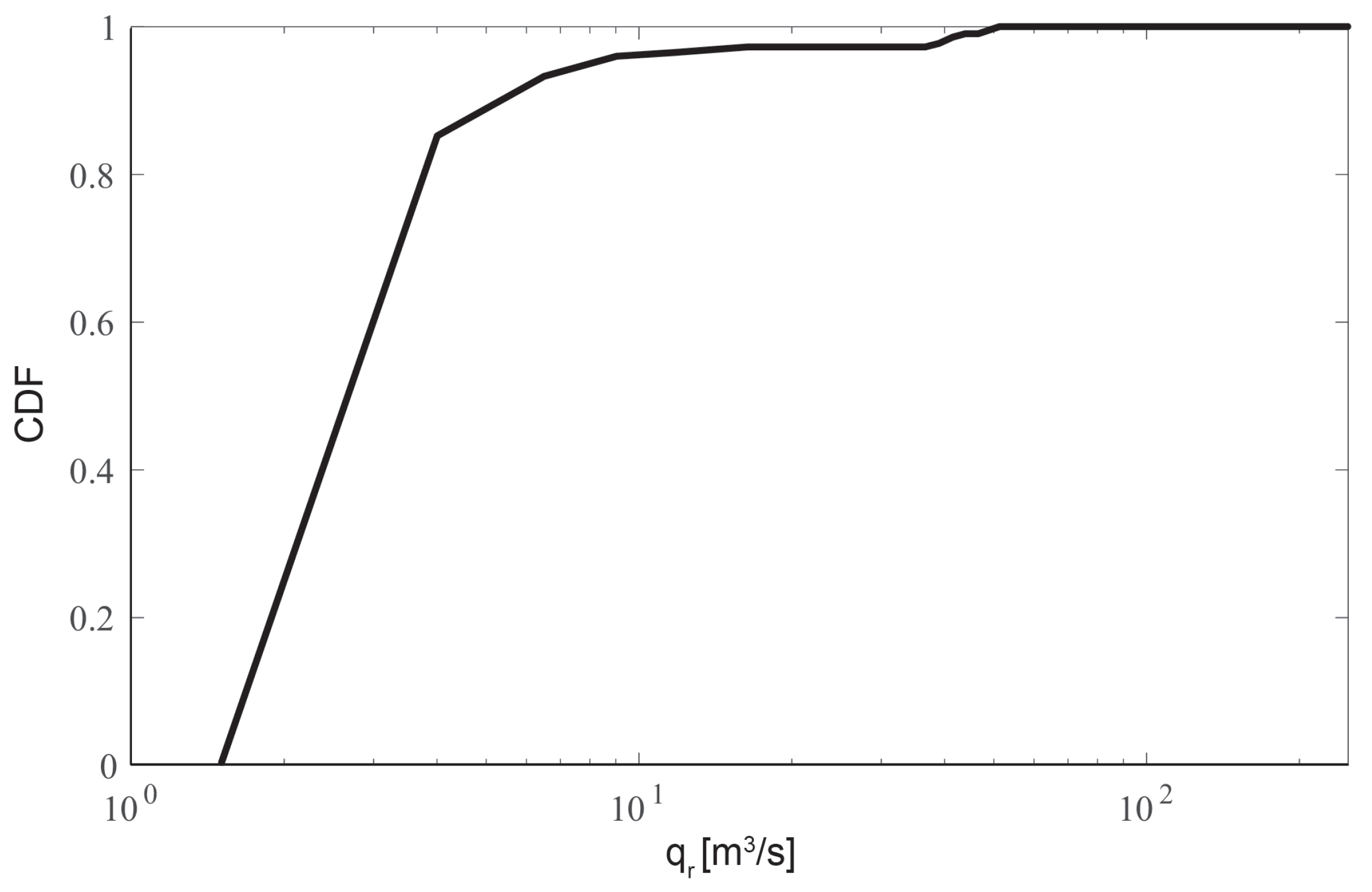
6. Results
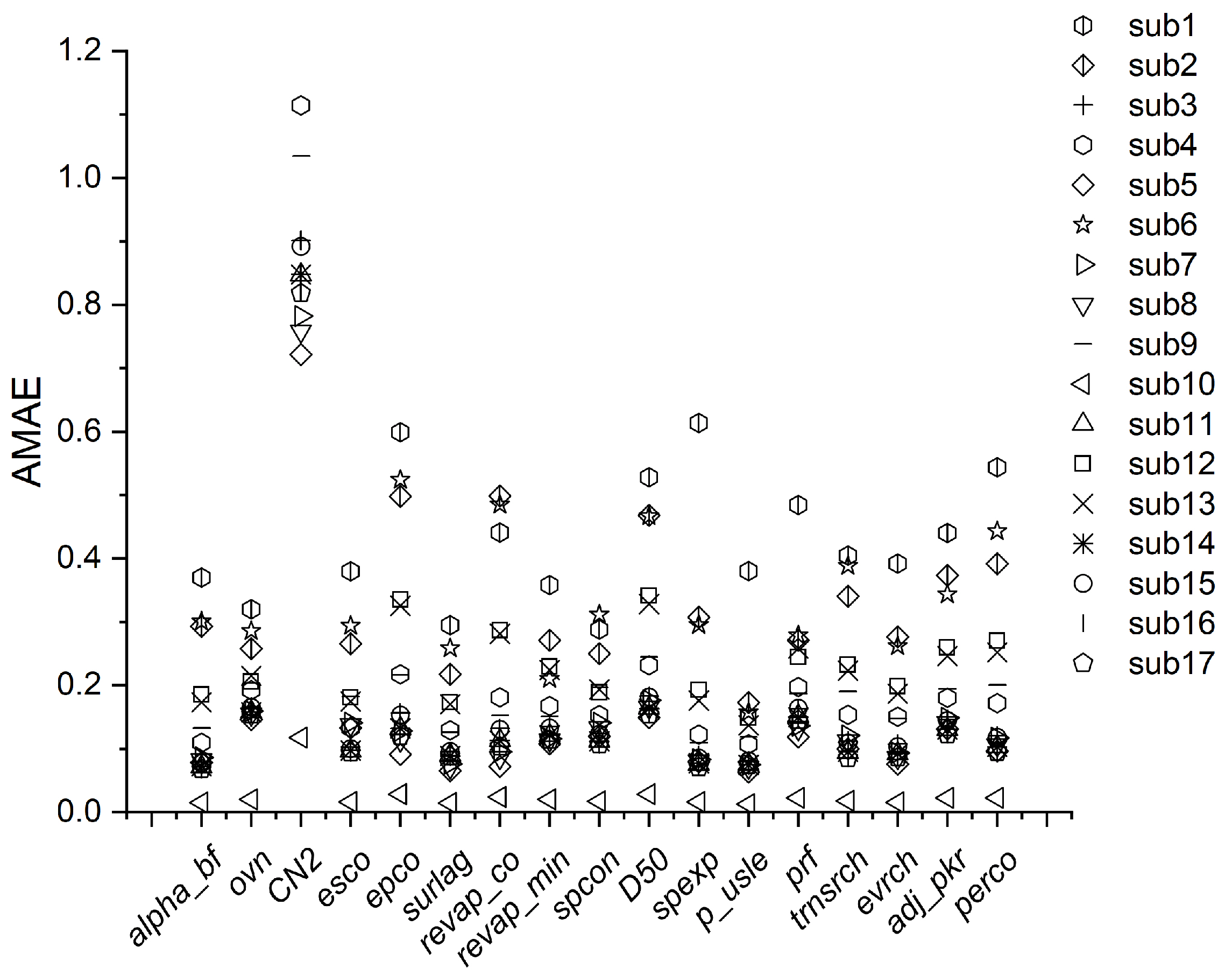
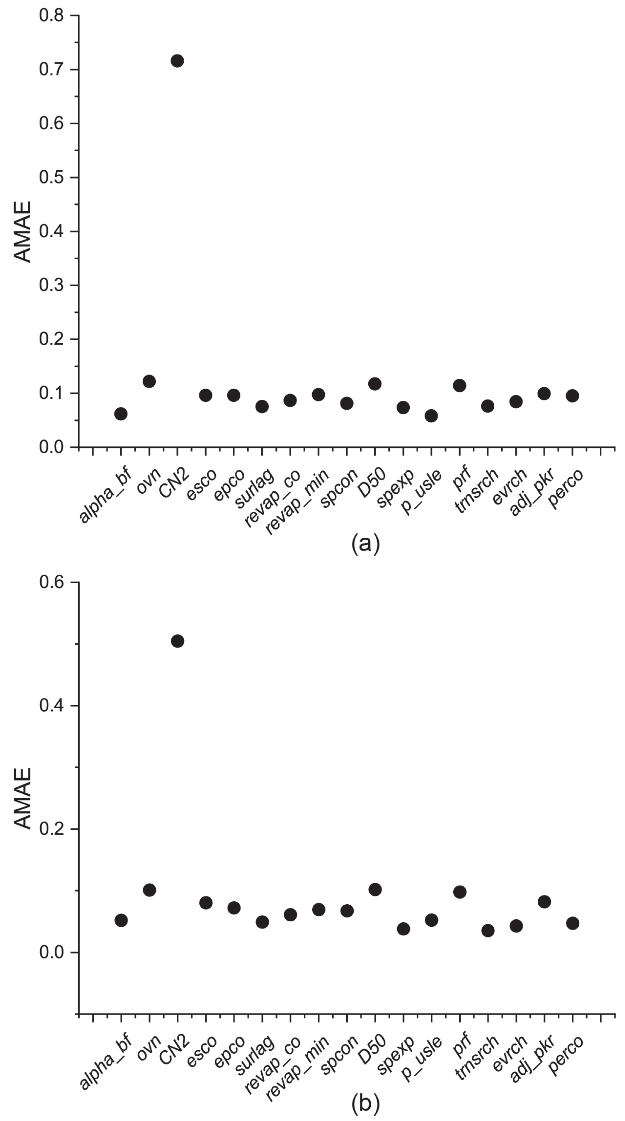
Sensitivity Analysis
7. Conclusions
Author Contributions
Funding
Institutional Review Board Statement
Informed Consent Statement
Data Availability Statement
Acknowledgments
Conflicts of Interest
Appendix A. Model Parameters
Appendix A.1. Surface Processes
Appendix A.2. Soil and Subsurface Flow
Appendix A.3. Erosion
References
- Mutunga, C.; Zulu, E.M.; De Souza, R.M. Population dynamics, climate change and sustainable development in Africa. 2012. Available online: https://www.africaportal.org/publications/population-dynamics-climate-change-and-sustainable-development-in-africa/ (accessed on 15 May 2021).
- Zeraebruk, K.N.; Mayabi, A.O.; Gathenya, J.M. Assessment of Water Resources and Analysis of Safe Yield and Reliability of Surface Water Reservoirs of Asmara Water Supply System. Environ. Nat. Resour. Res. 2017, 7, 45. [Google Scholar] [CrossRef] [Green Version]
- Tewolde, M.G.; Cabral, P. Urban sprawl analysis and modeling in Asmara, Eritrea. Remote Sens. 2011, 3, 2148–2165. [Google Scholar] [CrossRef] [Green Version]
- Polimi. VITAE. Available online: https://www.mecc.polimi.it/us/about-us/news/progetto-vitae-new-strategies-for-a-sustainable-valorisation-of-the-eritrean-heritage/ (accessed on 15 February 2022).
- Bortolotto, S.; Cattaneo, N.; Massa, S. Seasonal watercourses as a source of wealth and a cause of destruction: The water management in Adulis (Eritrea) in antiquity and today. Larhyss J. 2021, 47, 25–38. [Google Scholar]
- Bortolotto, S.; Cheli, F. Eritrean Mobility and Cultural Heritage. New Frontiers of the Horn of Africa. An overview of the project. E Motion Eritrean Mobil. Cult. Heritage. New Front. Horn Afr. 2021, 17, 23. [Google Scholar]
- Arnold, J.G.; Fohrer, N. SWAT2000: Current capabilities and research opportunities in applied watershed modelling. Hydrol. Process. Int. J. 2005, 19, 563–572. [Google Scholar] [CrossRef]
- Rockwood, D.M.; Davis, E.M.; Anderson, J.A. User Manual for COSSARR Model; US Army Engineer Division, North Pacific: Oregon, Portland, 1972. [Google Scholar]
- Sugawara, M. Tank model and its application to Bird Creek, Wollombi Brook, Bikin River, Kitsu River, Sanaga River and Nam Mune. Res. Notes Natl. Res. Cent. Disaster Prev. 1974, 11, 1–64. [Google Scholar]
- Hydrologic Engineering Center (US); Water Resources Support Center (US). HEC-1 Flood Hydrograph Package: Users Manual; US Army Corps of Engineers, Water Resources Support Center, Hydrologic: Fort Belvoir, VA, USA, 1981.
- Williams, J.; Hann, R. HYMO: Problem-oriented language for hydrologic modeling-User’s manual. USDA. ARS-S-9 1973, 45, 1–76. [Google Scholar]
- Abbott, M.; Bathurst, J.; Cunge, J.; O’connell, P.; Rasmussen, J. An introduction to the European Hydrological System—Systeme Hydrologique Europeen,“SHE”, 2: Structure of a physically-based, distributed modelling system. J. Hydrol. 1986, 87, 61–77. [Google Scholar] [CrossRef]
- Beven, K.; Calver, A.; Morris, E. The Institute of Hydrology Distributed Model; Institute of Hydrology: Wallingford, UK, 1987.
- Knisel, W.G. CREAMS: A Field Scale Model for Chemicals, Runoff, and Erosion from Agricultural Management Systems; Number 26; Department of Agriculture, Science and Education Administration: Hyattsville, MD, USA, 1980; pp. 1–113. [Google Scholar]
- Leonard, R.; Knisel, W.; Still, D. GLEAMS: Groundwater loading effects of agricultural management systems. Trans. ASAE 1987, 30, 1403–1418. [Google Scholar] [CrossRef]
- Williams, J.R.; Jones, C.; Dyke, P.T. A modeling approach to determining the relationship between erosion and soil productivity. Trans. ASAE 1984, 27, 129–0144. [Google Scholar] [CrossRef]
- Neitsch, S.L.; Arnold, J.G.; Kiniry, J.R.; Williams, J.R. Soil and Water Assessment Tool Theoretical Documentation Version 2009; Technical Report; Texas Water Resources Institute: College Station, TX, USA, 2011; pp. 1–618. [Google Scholar]
- Hussainzada, W.; Lee, H.S. Hydrological Modelling for Water Resource Management in a Semi-Arid Mountainous Region Using the Soil and Water Assessment Tool: A Case Study in Northern Afghanistan. Hydrology 2021, 8, 16. [Google Scholar] [CrossRef]
- Emiru, N.C.; Recha, J.W.; Thompson, J.R.; Belay, A.; Aynekulu, E.; Manyevere, A.; Demissie, T.D.; Osano, P.M.; Hussein, J.; Molla, M.B.; et al. Impact of Climate Change on the Hydrology of the Upper Awash River Basin, Ethiopia. Hydrology 2022, 9, 3. [Google Scholar] [CrossRef]
- Saade, J.; Atieh, M.; Ghanimeh, S.; Golmohammadi, G. Modeling Impact of Climate Change on Surface Water Availability Using SWAT Model in a Semi-Arid Basin: Case of El Kalb River, Lebanon. Hydrology 2021, 8, 134. [Google Scholar] [CrossRef]
- Ibrahim, B.; Wisser, D.; Barry, B.; Fowe, T.; Aduna, A. Hydrological predictions for small ungauged watersheds in the Sudanian zone of the Volta basin in West Africa. J. Hydrol. Reg. Stud. 2015, 4, 386–397. [Google Scholar] [CrossRef] [Green Version]
- Carannante, A.; Flaux, C.; Morhange, C.; Zazzaro, C. Adulis in its regional maritime context. apreliminary report of the 2015 field season. Newsl. Di Archeol. CISA 2015, 6, 279–294. [Google Scholar]
- Ogbazghi, W. Agro-climatic and environmental hazards and mitigation measures for the Northern and Southern Red Sea zone administrations of Eritrea. J. Eritrean Stud. 2018, 8, 85–131. [Google Scholar]
- Dile Yihun, T.S.R. QGIS Interface for SWAT+: QSWAT+; 2021; pp. 1–136. Available online: https://docplayer.net/204909159-Qgis-interface-for-swat-qswat.html (accessed on 15 May 2021).
- Tarboton, D. SOILGRIDS. Available online: https://soilgrids.org/ (accessed on 15 May 2021).
- Batjes, N.H.; Ribeiro, E.; Van Oostrum, A. Standardised soil profile data to support global mapping and modelling (WoSIS snapshot 2019). Earth Syst. Sci. Data 2020, 12, 299–320. [Google Scholar] [CrossRef] [Green Version]
- Wang, P.L.; Feddema, J.J. Linking global land use/land cover to hydrologic soil groups from 850 to 2015. Glob. Biogeochem. Cycles 2020, 34, e2019GB006356. [Google Scholar] [CrossRef]
- Campbell, G.S. Soil Physics with Basic, Transport Models for Soils-Plant Systems; Technical Report; Elsevier: Amsterdam, The Netherlands, 1985; Volume 14, pp. 1–150. [Google Scholar]
- Saha, S.; Moorthi, S.; Wu, X.; Wang, J.; Nadiga, S.; Tripp, P.; Behringer, D.; Hou, Y.T.; Chuang, H.Y.; Iredell, M.; et al. The NCEP climate forecast system version 2. J. Clim. 2014, 27, 2185–2208. [Google Scholar] [CrossRef]
- Fuka, D.R.; Walter, M.T.; MacAlister, C.; Degaetano, A.T.; Steenhuis, T.S.; Easton, Z.M. Using the Climate Forecast System Reanalysis as weather input data for watershed models. Hydrol. Process. 2014, 28, 5613–5623. [Google Scholar] [CrossRef]
- Tarboton, D. TauDEM. Available online: https://hydrology.usu.edu/taudem/taudem5/downloads.html (accessed on 15 May 2021).
- Jenkinson, A. The frequency distribution of the annual maximum (or minimum) values of meteorological events. QJ Roy. Meteor. Soc. 1955, 87, 158–171. [Google Scholar] [CrossRef]
- OriginPro, V. OriginLab Corporation; OriginLab Corporation Indicates: Northampton, MA, USA, 2016. [Google Scholar]
- Soil Conservation Service. National Engineering Handbook, Section 4, Hydrology; Soil Conservation Service: Washington, DC, USA, 1972; pp. 1–20.
- Monteith, J. Evaporation and the environment. Jawra J. Am. Water Resour. Assoc. 1965, 19, 205–234. [Google Scholar]
- Venetis, C. A study on the recession of unconfined acquifers. Int. Assoc. Sci. Hydrology. Bull. 1969, 14, 119–125. [Google Scholar] [CrossRef]
- Williams, J. Sediment routing for agricultural watersheds 1. JAWRA J. Am. Water Resour. Assoc. 1975, 11, 965–974. [Google Scholar] [CrossRef]
- Williams, J. Chapter 25: The EPIC model. Comput. Model. Watershed Hydrol. 1995, 909–1000. [Google Scholar]
- Bagnold, R. Bed load transport by natural rivers. Water Resour. Res. 1977, 13, 303–312. [Google Scholar] [CrossRef]
- Dell’Oca, A.; Riva, M.; Guadagnini, A. Moment-based metrics for global sensitivity analysis of hydrological systems. Hydrol. Earth Syst. Sci. 2017, 21, 6219–6234. [Google Scholar] [CrossRef] [Green Version]


| Data Type | Purpose | Provider | URL |
|---|---|---|---|
| DEM (digital elevation model) | Delineation of watershed of the area and stream network | NASA | https://search.earthdata.nasa.gov/, accessed on 15 May 2021 |
| Land cover map | Identification of the land use for each HRU of the watershed | FAO | https://www.fao.org/3/x0596e/x0596e00.htm, accessed on 15 May 2021 |
| Soil map | Identification of the soil type for the parameterization of infiltration, runoff and evapotranspiration fluxes | FAO | https://data.apps.fao.org/map/catalog/srv/ita/catalog.search#/metadata/ca4628f0-88fd-11da-a88f-000d939bc5d8, accessed on 15 May 2021 |
| Climatic data | Daily data of precipitation, wind, relative humidity, and solar radiation | National Centers for Environmental Prediction (NCEP) | https://globalweather.tamu.edu/, accessed on 15 May 2021 |
| Description FAO | Description SWAT | SWAT Code |
|---|---|---|
| Low sparse sHRUbs with herbaceous. SHRUbs density varies from 1 to 15% | Range grasses | RNGE |
| Very open sHRUbs with herbaceous from closed to open. The height of sHRUbs varies from 0.3 to 5 m. SHRUbs density varies from 40 to 65% | Range brush | RNGB |
| Needleleaved evergreen closed trees with sHRUbs | Forest evergreen | FRSE |
| Closed woody vegetation | Forest—mixed | FRST |
| Irrigated herbaceous crop, large to medium fields—cereal. Irrigated cereals crop. Fields density comprises from 20 to 49. Non-perennial river | Agriculture land—generic | AGRL |
| Sand | Rock sand | UIDU |
| Non-perennial river | Water | WATR |
| Code | Depth (cm) | Clay Content (%) | Sand Content (%) | Silt Content (%) | Textural Class | Hydrologic Soil Group |
|---|---|---|---|---|---|---|
| Bd31-2c-11 | 0-5 | 27.25 | 41.65 | 31.10 | Clay Loam | D |
| 5–15 | 28.41 | 40.91 | 30.68 | Clay Loam | D | |
| 15–30 | 32.44 | 38.21 | 29.35 | Clay Loam | D | |
| 30–60 | 36.56 | 35.26 | 28.18 | Clay Loam | D | |
| 60–100 | 36.57 | 35.26 | 28.17 | Clay Loam | D | |
| 100–200 | 35.56 | 36.32 | 28.12 | Clay Loam | D | |
| Bh13-2-3c | 0-5 | 29.11 | 41.92 | 28.97 | Clay Loam | D |
| 5–15 | 30.30 | 41.11 | 28.59 | Clay Loam | D | |
| 15–30 | 33.55 | 38.99 | 27.46 | Clay Loam | D | |
| 30–60 | 37.37 | 36.49 | 26.14 | Clay Loam | D | |
| 60–100 | 37.55 | 36.27 | 26.18 | Clay Loam | D | |
| 100–200 | 36.82 | 36.89 | 26.29 | Clay Loam | D | |
| Re16-b-235 | 0-5 | 25.56 | 44.32 | 30.12 | Loam | B |
| 5–15 | 27.19 | 43.49 | 29.32 | Clay Loam | D | |
| 15–30 | 29.67 | 41.72 | 28.61 | Clay Loam | D | |
| 30–60 | 30.37 | 41.30 | 28.33 | Clay Loam | D | |
| 60–100 | 30.78 | 40.52 | 28.70 | Clay Loam | D | |
| 100–200 | 29.55 | 41.77 | 28.68 | Clay Loam | D |
| Type Parameter | Name | Definition | Default Value | Range | Type Variation |
|---|---|---|---|---|---|
| Surface runoff | CN2 | SCS runoff curve number for moisture condition II | 59 | [−25%, 25%] | pctchg |
| surlag | Surface runoff lag coefficient | 4 | [−25%, 25%] | pctchg | |
| Channel | ovn | Manning’s roughness coefficient | 0.365 | [−25%, 25%] | pctchg |
| trnsrch | Fraction of transmission losses from main channel that enter deep aquifer | 0 | [−25%, 25%] | pctchg | |
| Evapo-transpiration | esco | Soil evaporation compensation factor | 0.95 | [0, 1] | absval |
| epco | Plant evaporation compensation factor | 1 | [0, 1] | absval | |
| evrch | Reach evaporation adjustment factor | 1 | [0, 1] | absval | |
| Percolation | perco | Percolation coefficient-adjusts soil moisture for percolation to occur | 1 | [−25%, 25%] | pctchg |
| Type Parameter | Name | Definition | Default Value | Range | Type Variation |
|---|---|---|---|---|---|
| Sediments | spcon | Linear parameter for calculating the maximum amount of sediment that can be re-entrained | 0.0001 | [−25%, 25%] | pctchg |
| D50 | Median particle diameter of sediment (μm) | 12 | [−25%, 25%] | pctchg | |
| spexp | Exponent parameter for calculating sediment reentrained in channel sediment routing | 1 | [−25%, 25%] | pctchg | |
| p_usle | USLE equation support practice factor | 0.875 | [−25%, 25%] | pctchg | |
| prf | Peak rate adjustment factor for sediment routing in the main channel | 1 | [−25%, 25%] | pctchg | |
| adj_pkr | Peak rate adjustment factor for sediment routing in the subbasin (tributary channels) | 1 | [0.5, 1] | absval | |
Groundwater | revap_co | Groundwater revap coefficient | 0.02 | [−25%, 25%] | pctchg |
| revap_min | Threshold depth of water in the shallow aquifer for revap to occur (mm) | 5 | [−25%, 25%] | pctchg | |
| alpha_bf | Base flow alpha factor (days) | 0.05 | [−25%, 25%] | pctchg |
Publisher’s Note: MDPI stays neutral with regard to jurisdictional claims in published maps and institutional affiliations. |
© 2022 by the authors. Licensee MDPI, Basel, Switzerland. This article is an open access article distributed under the terms and conditions of the Creative Commons Attribution (CC BY) license (https://creativecommons.org/licenses/by/4.0/).
Share and Cite
Baioni, E.; Porta, G.M.; Cattaneo, N.; Guadagnini, A. Assessment of Hydrological Processes in an Ungauged Catchment in Eritrea. Hydrology 2022, 9, 68. https://doi.org/10.3390/hydrology9050068
Baioni E, Porta GM, Cattaneo N, Guadagnini A. Assessment of Hydrological Processes in an Ungauged Catchment in Eritrea. Hydrology. 2022; 9(5):68. https://doi.org/10.3390/hydrology9050068
Chicago/Turabian StyleBaioni, Elisa, Giovanni Michele Porta, Nelly Cattaneo, and Alberto Guadagnini. 2022. "Assessment of Hydrological Processes in an Ungauged Catchment in Eritrea" Hydrology 9, no. 5: 68. https://doi.org/10.3390/hydrology9050068
APA StyleBaioni, E., Porta, G. M., Cattaneo, N., & Guadagnini, A. (2022). Assessment of Hydrological Processes in an Ungauged Catchment in Eritrea. Hydrology, 9(5), 68. https://doi.org/10.3390/hydrology9050068