
Regional Ombrian Curves: Design Rainfall Estimation for a Spatially Diverse Rainfall Regime


Abstract
1. Introduction
- (a)
- the at-site, independent fitting approach, which consists of separately fitting the curves to multiple gauged sites and using spatial interpolation methods to map the parameters over the whole region.
- (b)
- the regional, simultaneous fitting approach, which consists of appropriately pooling the data together and obtaining a single model valid over the entire area, which is, in essence, the inverse approach to (a).
2. Methodology
2.1. Mathematical Form of the Ombrian Relationship
- , and hence we can set the quantity in Equation (1).
- , and thus we can neglect the latter term in their sum.
- we select the generalized Cauchy-type model for the climacogram:where and are scale parameters, with dimensions of time and , respectively, and , are dimensionless parameters in the interval (0, 1), controlling the long-range (Hurst-Kolmogorov dynamics) and local scaling of the process (fractal behavior) of the process, respectively. For we take the neutral value as default. We note though that if the focus is on even smaller temporal scales, this value () can be inappropriate.
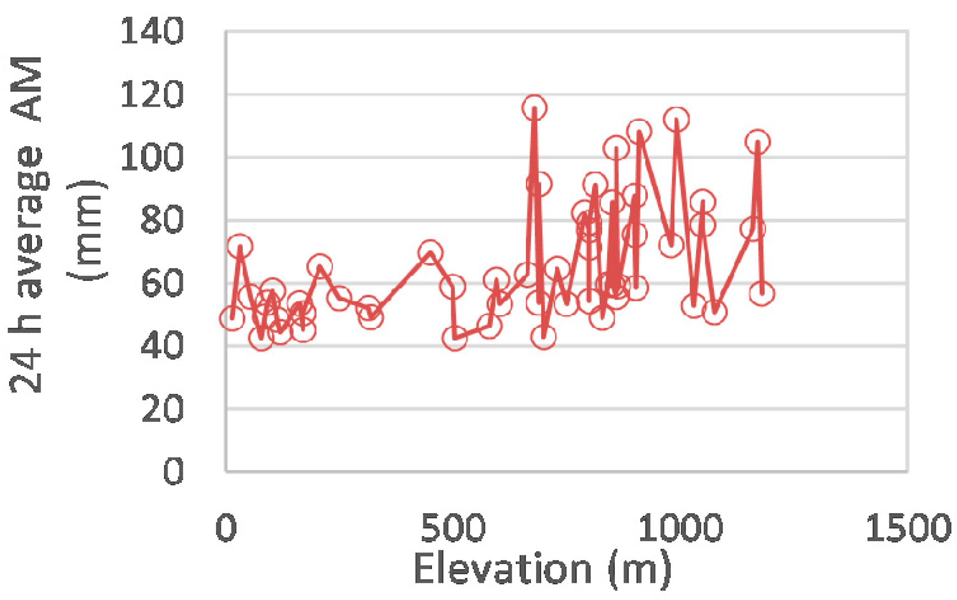
2.2. Regionalization Method: Bilinear Surface Smoothing Models for the 24 h Average Annual Rainfall Maxima
2.3. Bilinear Surface Smoothing Model Parameters Estimation
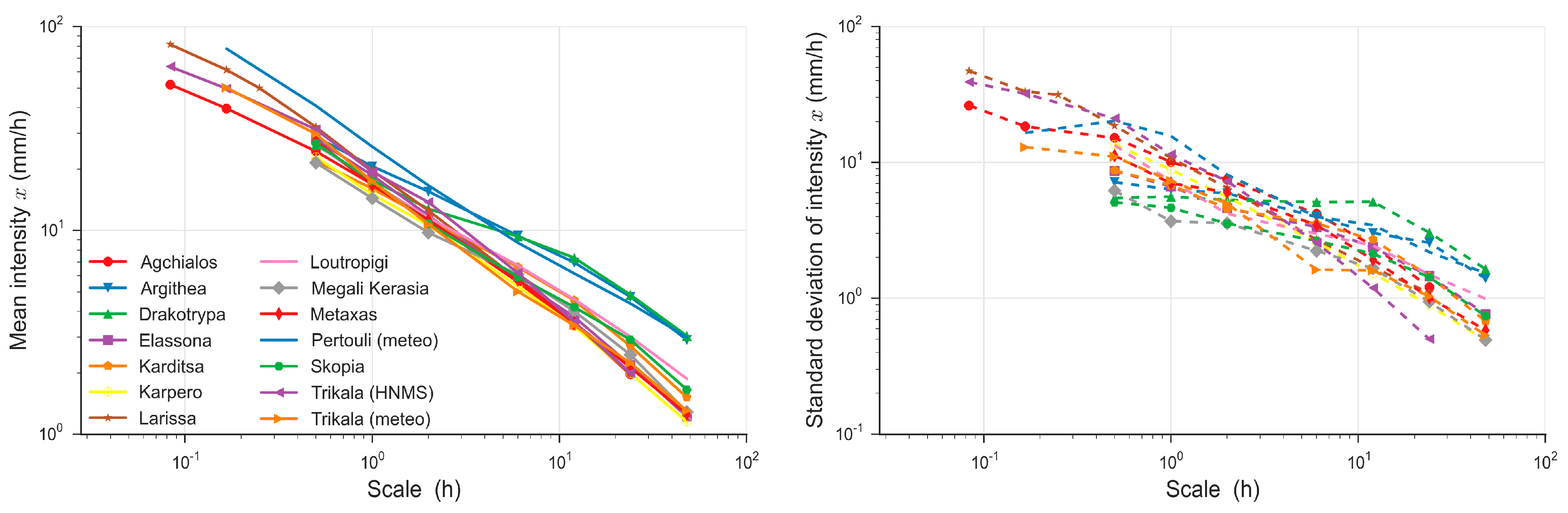
2.4. Timescale Parameters Estimation
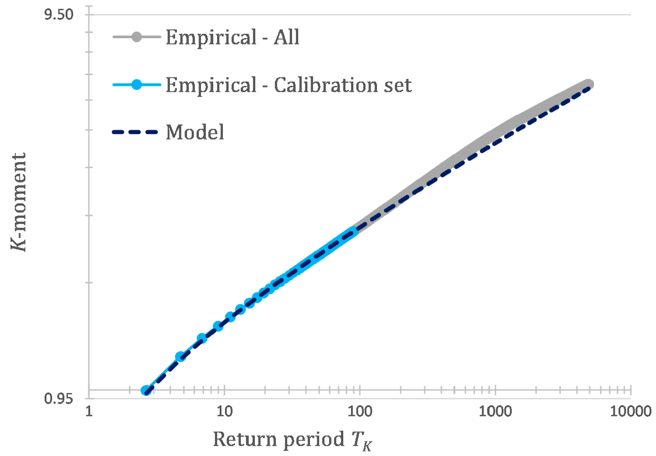
2.5. Regional Estimation of Distribution Parameters through K-Moments
- For we set .
- For the following approximation is used. We estimate the equivalent Hurst parameter , based on the spatial correlation of the stations :Based on the estimated the following coefficient is used for bias correction, :Then the modified orders of the moments are obtained as:and their corresponding return periods are adjusted accordingly based on Equation (23).
3. Data
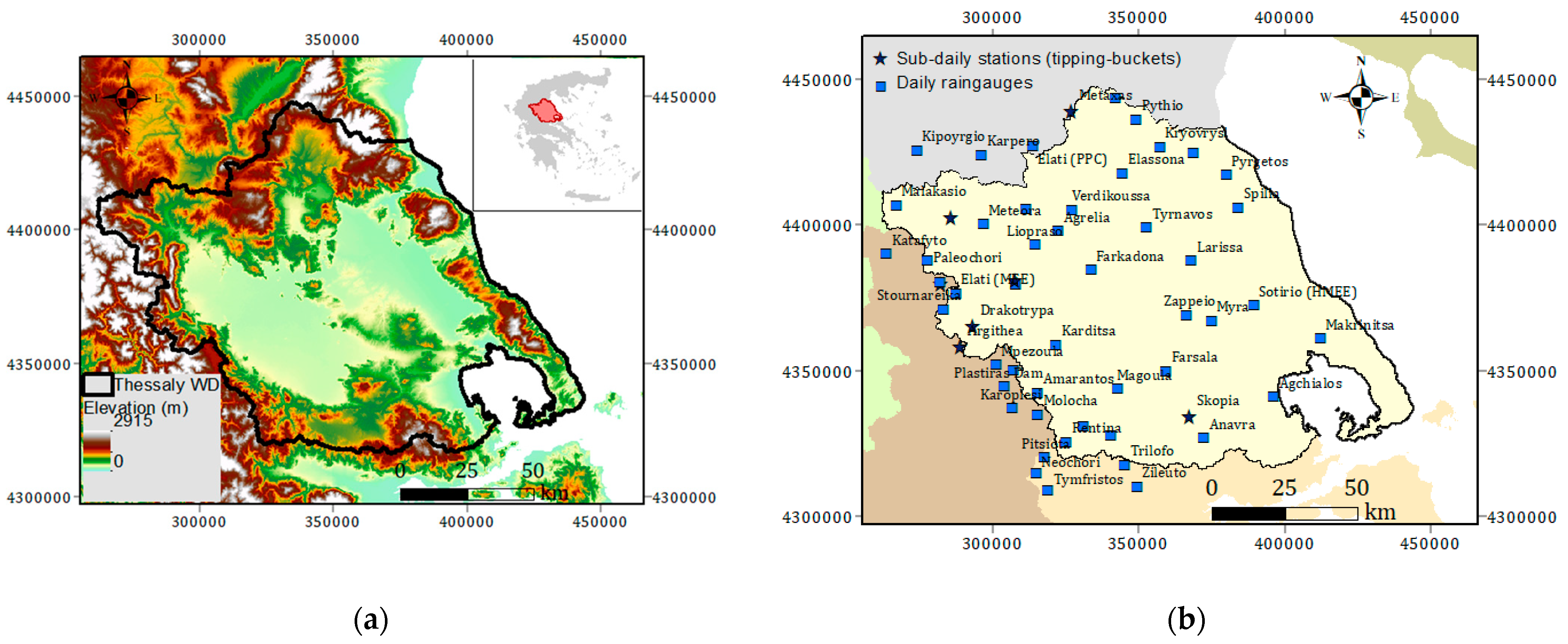
3.1. Study Area
3.2. Data Processing and Quality Control
4. Results
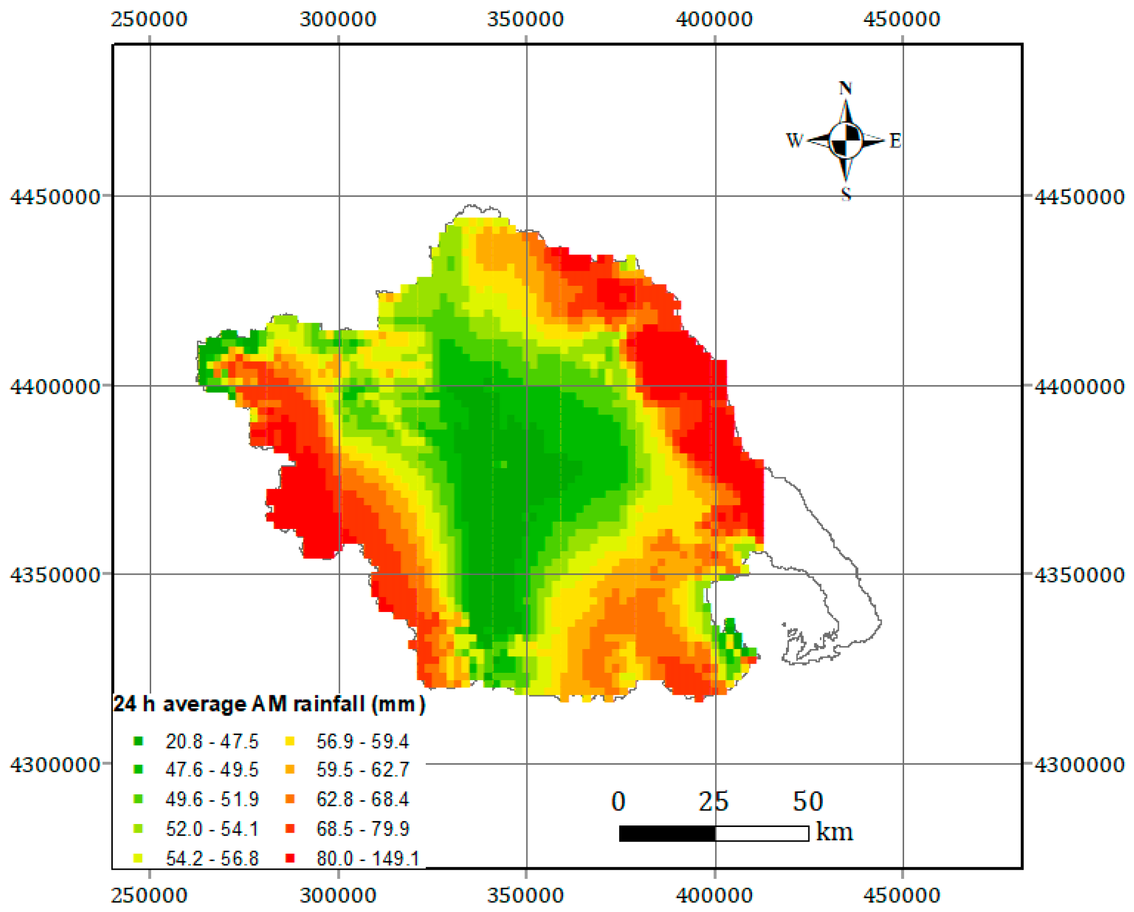
4.1. Fitting of the Bilinear Surface Smoothing Models
4.2. Construction of the Regional Ombrian Curves
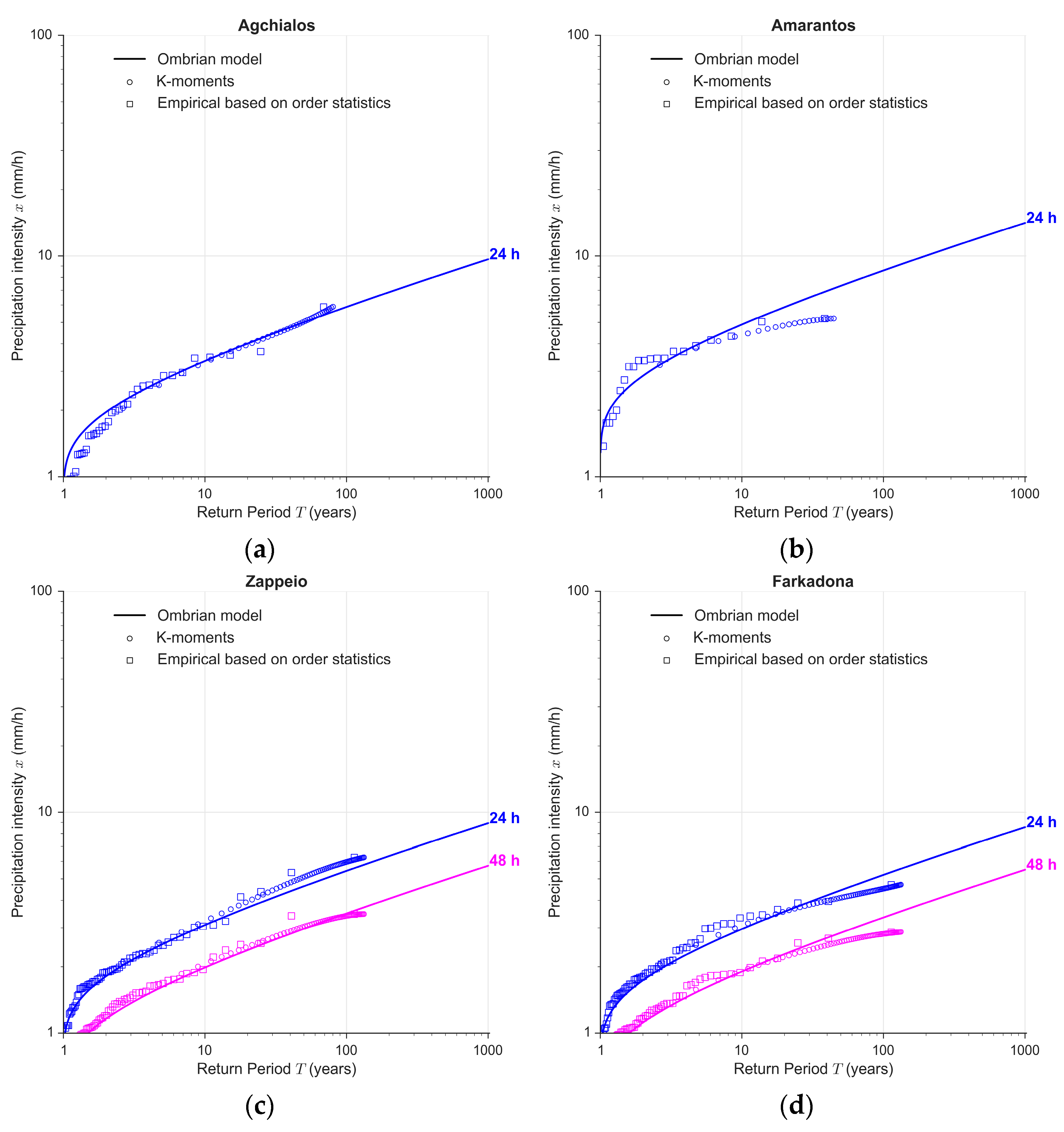
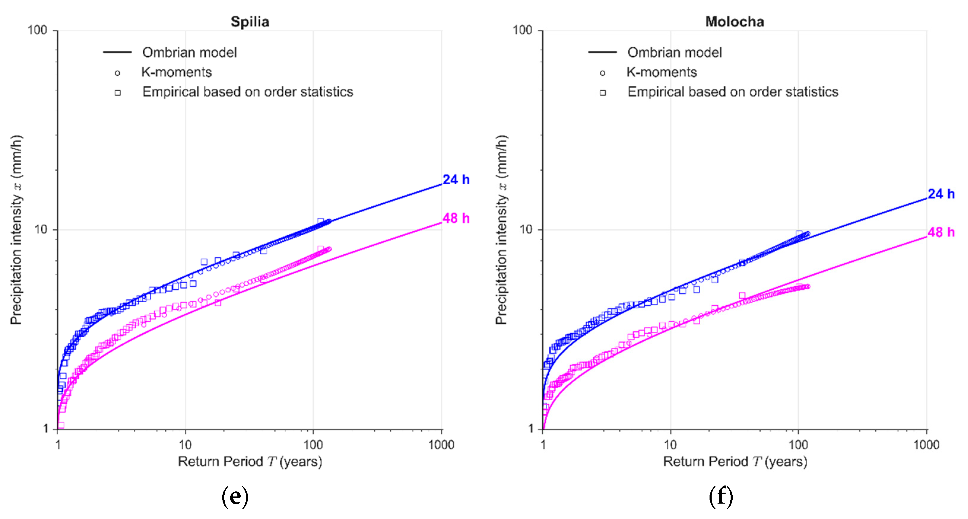
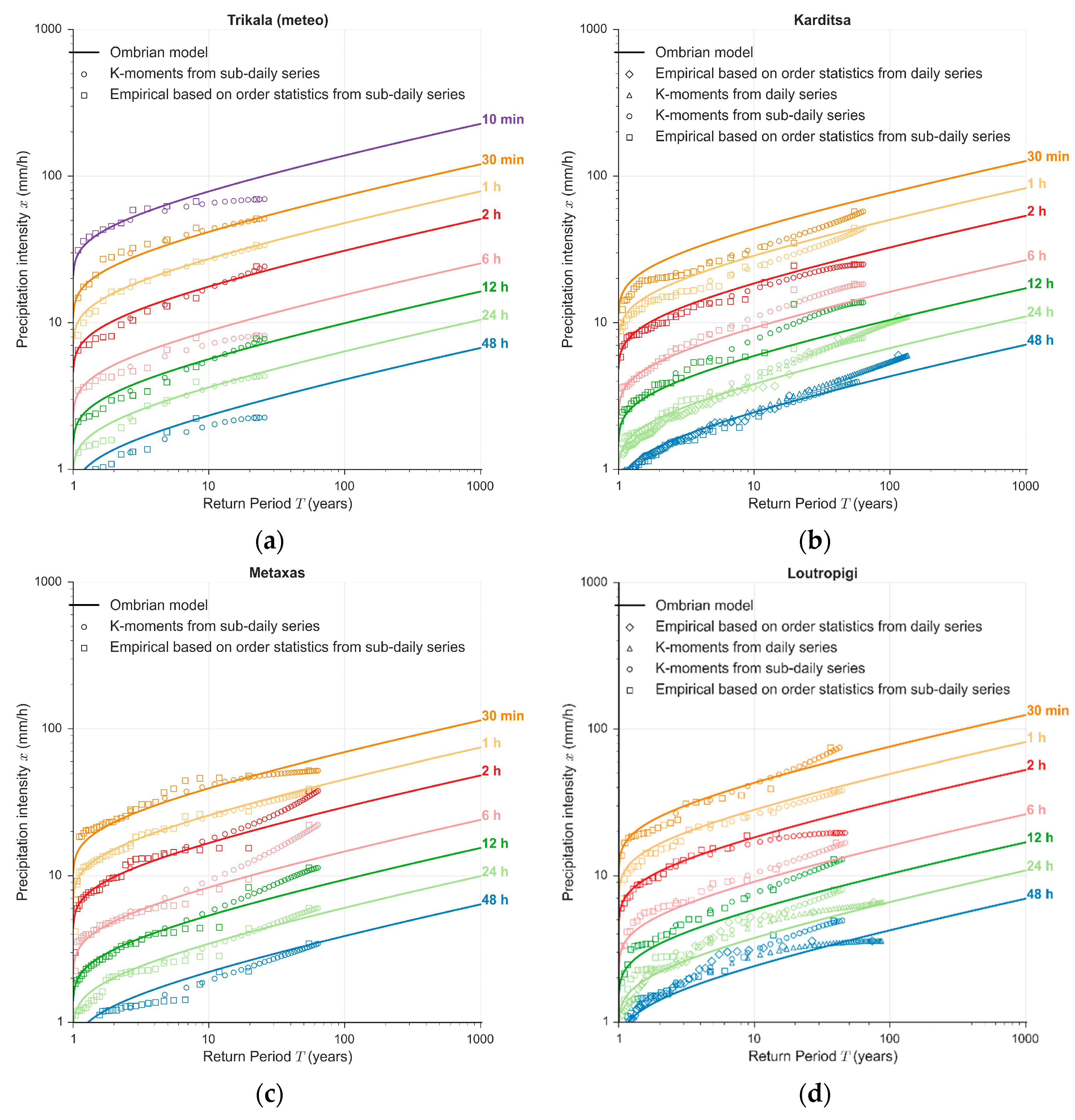
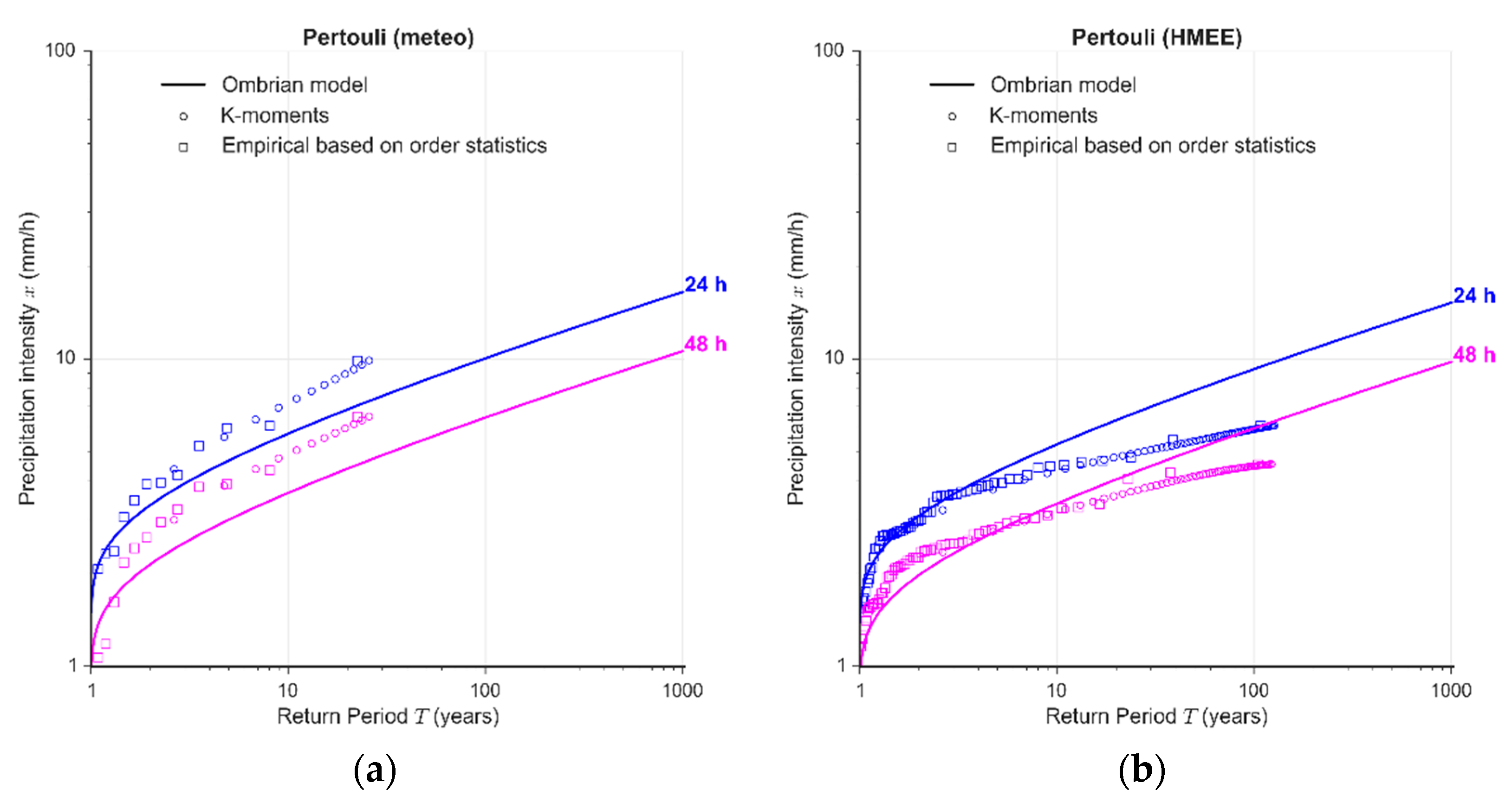
4.3. At-Site Verification
5. Discussion and Conclusions
Supplementary Materials
Author Contributions
Funding
Institutional Review Board Statement
Informed Consent Statement
Data Availability Statement
Acknowledgments
Conflicts of Interest
References
- Lesher, J.H. Saphêneia in Aristotle: “Clarity”, “Precision”, and “Knowledge”. Apeiron 2010, 43, 143–156. [Google Scholar] [CrossRef]
- Koutsoyiannis, D. Stochastics of Hydroclimatic Extremes—A Cool Look at Risk; Kallipos: Athens, Greece, 2021; 333p, ISBN 978-618-85370-0-2. Available online: https://repository.kallipos.gr/handle/11419/6522 (accessed on 1 April 2021).
- Koutsoyiannis, D.; Iliopoulou, T. Ombrian curves advanced to stochastic modelling of rainfall intensity. In Rainfall: Modeling, Measurement and Applications; Elsevier: Amsterdam, The Netherlands, 2022; pp. 261–284. [Google Scholar] [CrossRef]
- Iliopoulou, T.; Koutsoyiannis, D. PythOm: A python toolbox implementing recent advances in rainfall intensity (ombrian) curves. Eur. Geosci. Union Gen. Assem. 2021, EGU21-389. [Google Scholar] [CrossRef]
- Papalexiou, S.M.; Koutsoyiannis, D. Ombrian curves in a maximum entropy framework. Eur. Geosci. Union Gen. Assem. 2008, 10, 00702. [Google Scholar]
- Sherman, C.W. Frequency and intensity of excessive rainfalls at Boston, Massachusetts. Trans. Am. Soc. Civ. Eng. 1931, 95, 951–960. [Google Scholar] [CrossRef]
- Bernard, M.M. Formulas for rainfall intensities of long duration. Trans. Am. Soc. Civ. Eng. 1932, 96, 592–606. [Google Scholar] [CrossRef]
- Koutsoyiannis, D.; Kozonis, D.; Manetas, A. A mathematical framework for studying rainfall intensity-duration-frequency relationships. J. Hydrol. 1998, 206, 118–135. [Google Scholar] [CrossRef]
- Veneziano, D.; Furcolo, P. Multifractality of rainfall and scaling of intensity-duration-frequency curves. Water Resour. Res. 2002, 38, 42-1–42-12. [Google Scholar] [CrossRef]
- Langousis, A.; Veneziano, D. Intensity-duration-frequency curves from scaling representations of rainfall. Water Resour. Res. 2007, 43, 1306. [Google Scholar] [CrossRef]
- Svensson, C.; Jones, D.A. Review of rainfall frequency estimation methods. J. Flood Risk Manag. 2010, 3, 296–313. [Google Scholar] [CrossRef]
- Hershfield, D.M. Rainfall Frequency Atlas of the United States for Durations From 30 Minutes to 24 Hours and Return Periods From l to 100 Years; US Weather Bureau Technical Paper 40; U.S. Weather Bureau: Washington, DC, USA, 1961; Volume 40, pp. 1–61.
- Hogg, W.D.; Carr, D.A.; Routledge, B. Rainfall Intensity-Duration Frequency Values for Canadian Locations; Environment Canada, Atmospheric Environment Service: Downsview, ON, Canada, 1985. [Google Scholar]
- Borga, M.; Vezzani, C.; Dalla Fontana, G. Regional rainfall depth–duration–frequency equations for an alpine region. Nat. Hazards 2005, 36, 221–235. [Google Scholar] [CrossRef]
- Malamos, N.; Koutsoyiannis, D. Field survey and modelling of irrigation water quality indices in a Mediterranean island catchment: A comparison between spatial interpolation methods. Hydrol. Sci. J. 2018, 63, 1447–1467. [Google Scholar] [CrossRef]
- Oliver, M.A.; Webster, R. A tutorial guide to geostatistics: Computing and modelling variograms and kriging. Catena 2014, 113, 56–69. [Google Scholar] [CrossRef]
- Li, J.; Heap, A.D. Spatial interpolation methods applied in the environmental sciences: A review. Environ. Model. Softw. 2014, 53, 173–189. [Google Scholar] [CrossRef]
- Malamos, N.; Koutsoyiannis, D. Bilinear surface smoothing for spatial interpolation with optional incorporation of an explanatory variable. Part 1: Theory. Hydrol. Sci. J. 2016, 61, 519–526. [Google Scholar] [CrossRef]
- Malamos, N.; Koutsoyiannis, D. Bilinear surface smoothing for spatial interpolation with optional incorporation of an explanatory variable. Part 2: Application to synthesized and rainfall data. Hydrol. Sci. J. 2016, 61, 527–540. [Google Scholar] [CrossRef]
- Hosking, J.R.M.; Wallis, J.R. Regional Frequency Analysis: An Approach Based on L-Moments; Cambridge University Press: Cambridge, UK, 1997. [Google Scholar] [CrossRef]
- Hosking, J.R. L-moments: Analysis and estimation of distributions using linear combinations of order statistics, J.R. Stat. Soc. Ser. B Stat. Methodol. 1990, 52, 105–124. [Google Scholar] [CrossRef]
- Hosking, J.R.M.; Wallis, J.R. The effect of intersite dependence on regional flood frequency analysis. Water Resour. Res. 1988, 24, 588–600. [Google Scholar] [CrossRef]
- Koutsoyiannis, D. Knowable moments for high-order stochastic characterization and modelling of hydrological processes. Hydrol. Sci. J. 2019, 64, 19–33. [Google Scholar] [CrossRef]
- Weinmann, P.E.; Nandakumar, N.; Siriwardena, L.; Mein, R.G.; Nathan, R.J. Estimation of rare design rainfalls for Victoria using the CRC-FORGE methodology. In Water 99: Joint Congress; 25th Hydrology & Water Resources Symposium, 2nd International Conference on Water Resources & Environment Research; Handbook and Proceedings; Institution of Engineers: Barton, Australia, 1999; p. 284. [Google Scholar]
- Claps, P.; Ganora, D.; Mazzoglio, P. Rainfall regionalization techniques. In Rainfall: Modeling, Measurement and Applications; Elsevier: Amsterdam, The Netherlands, 2022; pp. 327–350. [Google Scholar] [CrossRef]
- Hailegeorgis, T.T.; Thorolfsson, S.T.; Alfredsen, K. Regional frequency analysis of extreme precipitation with consideration of uncertainties to update IDF curves for the city of Trondheim. J. Hydrol. 2013, 498, 305–318. [Google Scholar] [CrossRef]
- Aron, G.; Wall, D.J.; White, E.L.; Dunn, C.N. Regional rainfall intensity-duration-frequency curves for Pennsylvania 1. JAWRA J. Am. Water Resour. Assoc. 1987, 23, 479–485. [Google Scholar] [CrossRef]
- Trefry, C.M.; Watkins, D.W., Jr.; Johnson, D. Regional rainfall frequency analysis for the state of Michigan. J. Hydrol. Eng. 2005, 10, 437–449. [Google Scholar] [CrossRef]
- Dalrymple, T. Flood-Frequency Analyses. Manual of Hydrology: Part 3. Flood-Flow Techniques; USGPO: Washington, DC, USA, 1960; Volume 80. [CrossRef]
- Burn, D.H. An appraisal of the “region of influence” approach to flood frequency analysis. Hydrol. Sci. J. 1990, 35, 149–165. [Google Scholar] [CrossRef]
- Faulkner, D.S.; Prudhomme, C. Mapping an index of extreme rainfall across the UK. Hydrol. Earth Syst. Sci. 1998, 2, 183–194. [Google Scholar] [CrossRef]
- Deidda, R.; Hellies, M.; Langousis, A. A critical analysis of the shortcomings in spatial frequency analysis of rainfall extremes based on homogeneous regions and a comparison with a hierarchical boundaryless approach. Stoch. Environ. Res. Risk Assess. 2021, 35, 2605–2628. [Google Scholar] [CrossRef]
- Dimitriadis, P.; Koutsoyiannis, D.; Iliopoulou, T.; Papanicolaou, P. A global-scale investigation of stochastic similarities in marginal distribution and dependence structure of key hydrological-cycle processes. Hydrology 2021, 8, 59. [Google Scholar] [CrossRef]
- Glynis, K.G.; Iliopoulou, T.; Dimitriadis, P.; Koutsoyiannis, D. Stochastic investigation of daily air temperature extremes from a global ground station network. Stoch. Environ. Res. Risk Assess. 2021, 35, 1585–1603. [Google Scholar] [CrossRef]
- Koutsoyiannis, D.; Dimitriadis, P. Towards generic simulation for demanding stochastic processes. Sci 2021, 3, 34. [Google Scholar] [CrossRef]
- Koutsoyiannis, D. An entropic-stochastic representation of rainfall intermittency: The origin of clustering and persistence. Water Resour. Res. 2006, 42, W01401. [Google Scholar] [CrossRef]
- Koutsoyiannis, D. Statistics of extremes and estimation of extreme rainfall: II. Empirical investigation of long rainfall records/Statistiques de valeurs extrêmes et estimation de précipitations extrêmes: II. Recherche empirique sur de longues séries de précipitations. Hydrol. Sci. J. 2004, 49, 591–610. [Google Scholar] [CrossRef]
- Koutsoyiannis, D.; Papalexiou, S.M. Extreme rainfall: Global perspective. In Handbook of Applied Hydrology; McGraw-Hill: New York, NY, USA, 2017; pp. 74.1–74.16. [Google Scholar]
- Iliopoulou, T.; Koutsoyiannis, D.; Montanari, A. Characterizing and modeling seasonality in extreme rainfall. Water Resour. Res. 2018, 54, 6242–6258. [Google Scholar] [CrossRef]
- Koutsoyiannis, D. Broken line smoothing: A simple method for interpolating and smoothing data series. Environ. Model. Softw. 2000, 15, 139–149. [Google Scholar] [CrossRef][Green Version]
- Malamos, N.; Koutsoyiannis, D. Broken line smoothing for data series interpolation by incorporating an explanatory variable with denser observations: Application to soil-water and rainfall data. Hydrol. Sci. J. 2015, 60, 468–481. [Google Scholar] [CrossRef]
- Wahba, G.; Wendelberger, J. Some New Mathematical Methods for Variational Objective Analysis Using Splines and Cross Validation. Mon. Weather. Rev. 1980, 108, 1122–1143. [Google Scholar] [CrossRef]
- Jarvis, A.; Reuter, H.I.; Nelson, A.; Guevara, E. Hole-Filled SRTM for the Globe Version 4. 2008. Available online: http://srtm.csi.cgiar.org (accessed on 27 November 2021).
- Greenwood, J.A.; Landwehr, J.M.; Matalas, N.C.; Wallis, J.R. Probability weighted moments: Definition and relation to parameters of several distributions expressable in inverse form. Water Resour. Res. 1979, 15, 1049–1054. [Google Scholar] [CrossRef]
- Mimikou, M.; Koutsoyiannis, D. Extreme floods in Greece: The case of 1994. In Proceedings of the US-ITALY Research Workshop on the Hydrometeorology, Impacts, and Management of Extreme Floods, Perugia, Italy, 13–17 November 1995. [Google Scholar]
- Bathrellos, G.D.; Skilodimou, H.D.; Soukis, K.; Koskeridou, E. Temporal and spatial analysis of flood occurrences in the drainage basin of pinios river (thessaly, central greece). Land 2018, 7, 106. [Google Scholar] [CrossRef]
- Koutsoyiannis, D.; Mamassis, N.; Efstratiadis, A.; Zarkadoulas, N.; Markonis, Y. Floods in Greece, in Changes of Flood Risk in Europe; Wallingford—International Association of Hydrological Sciences; IAHS Press: Wallingford, UK, 2012; pp. 238–256. [Google Scholar]
- Loukas, A.; Vasiliades, L. Probabilistic analysis of drought spatiotemporal characteristics in Thessaly region, Greece. Nat. Hazards Earth Syst. Sci. 2004, 4, 719–731. [Google Scholar] [CrossRef]
- Lagouvardos, K.; Kotroni, V.; Bezes, A.; Koletsis, I.; Kopania, T.; Lykoudis, S.; Mazarakis, N.; Papagiannaki, K.; Vougioukas, S. The automatic weather stations NOANN network of the National Observatory of Athens: Operation and database. Geosci. Data J. 2017, 4, 4–16. [Google Scholar] [CrossRef]
- Hersfield, D.M.; Wilson, W.T. Generalizing of rainfall-intensity-frequency data. AIHS. Gen. Ass. Tor. 1957, 1, 499–506. [Google Scholar]
- Pasculli, A.; Longo, R.; Sciarra, N.; Di Nucci, C. Surface Water Flow Balance of a River Basin Using a Shallow Water Approach and GPU Parallel Computing; Pescara River (Italy) as Test Case. Water 2022, 14, 234. [Google Scholar] [CrossRef]
- Koutsoyiannis, D. An open letter to the Editor of Frontiers. Researchgate 2021. [Google Scholar] [CrossRef]


| Spatial Smoothing Model | BSS | BSSE |
|---|---|---|
| Parameters | = 0.005 | = 0.451 |
| A. All data | ||
| RMSE (mm) | 9.0 | 7.0 |
| MAE (mm) | 7.3 | 5.3 |
| Β. Leave-one-out cross validation | ||
| RMSE (mm) | 12.5 | 10.8 |
| MAE (mm) | 9.8 | 8.1 |
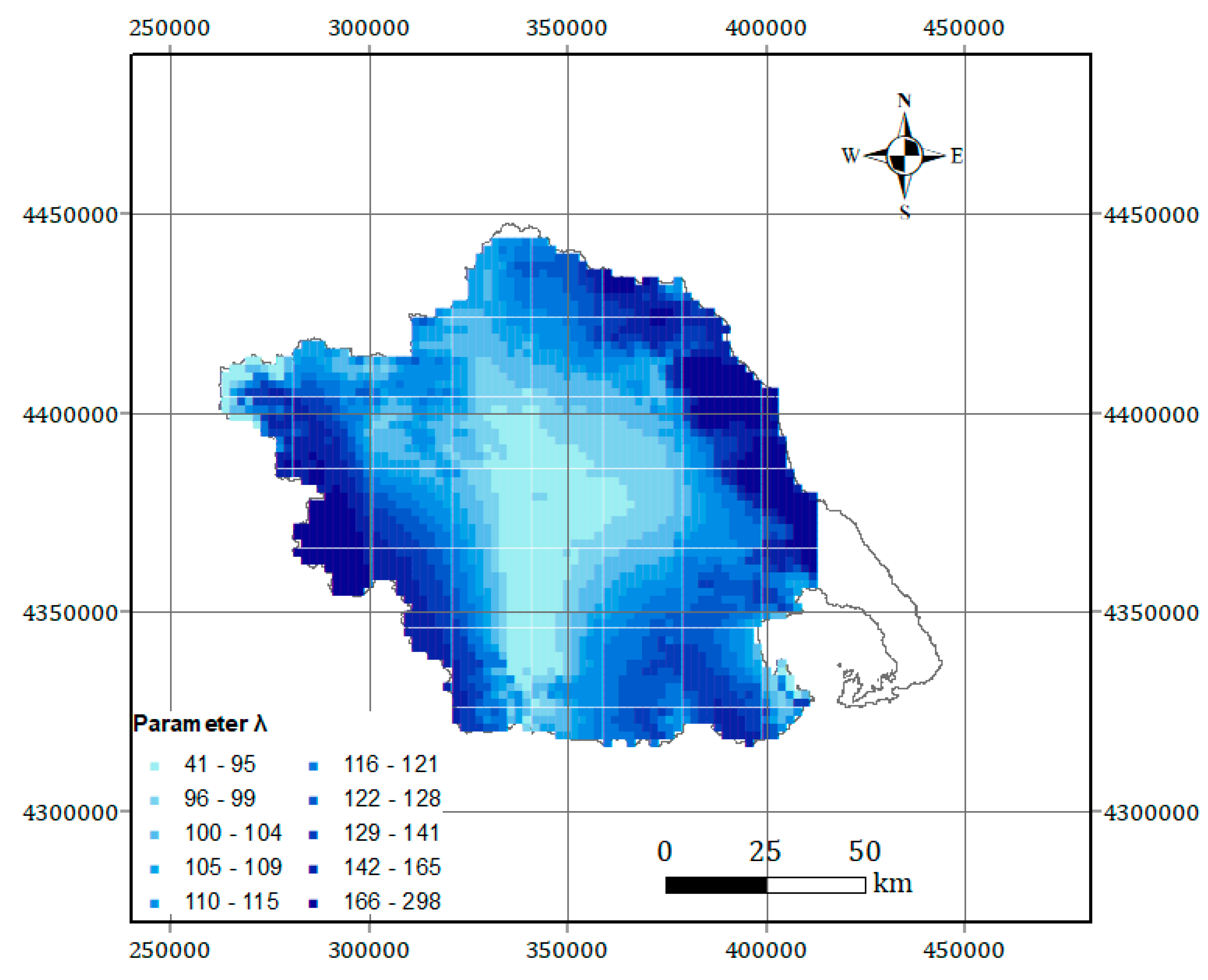
| α (h) | η (-) | ξ (-) | β (years) | λ (mm/h) |
|---|---|---|---|---|
| 0.03 | 0.64 | 0.18 | 0.013 | Geographic distribution shown in Figure 6 for all grid points. |
Publisher’s Note: MDPI stays neutral with regard to jurisdictional claims in published maps and institutional affiliations. |
© 2022 by the authors. Licensee MDPI, Basel, Switzerland. This article is an open access article distributed under the terms and conditions of the Creative Commons Attribution (CC BY) license (https://creativecommons.org/licenses/by/4.0/).
Share and Cite
Iliopoulou, T.; Malamos, N.; Koutsoyiannis, D. Regional Ombrian Curves: Design Rainfall Estimation for a Spatially Diverse Rainfall Regime. Hydrology 2022, 9, 67. https://doi.org/10.3390/hydrology9050067
Iliopoulou T, Malamos N, Koutsoyiannis D. Regional Ombrian Curves: Design Rainfall Estimation for a Spatially Diverse Rainfall Regime. Hydrology. 2022; 9(5):67. https://doi.org/10.3390/hydrology9050067
Chicago/Turabian StyleIliopoulou, Theano, Nikolaos Malamos, and Demetris Koutsoyiannis. 2022. "Regional Ombrian Curves: Design Rainfall Estimation for a Spatially Diverse Rainfall Regime" Hydrology 9, no. 5: 67. https://doi.org/10.3390/hydrology9050067
APA StyleIliopoulou, T., Malamos, N., & Koutsoyiannis, D. (2022). Regional Ombrian Curves: Design Rainfall Estimation for a Spatially Diverse Rainfall Regime. Hydrology, 9(5), 67. https://doi.org/10.3390/hydrology9050067