Abstract
Hurst’s seminal characterisation of long-term persistence (LTP) in geophysical records more than seven decades ago continues to inspire investigations into the Hurst phenomenon, not just in hydrology and climatology, but in many other scientific fields. Here, we present a new theoretical development based on stochastic Hurst–Kolmogorov (HK) dynamics that explains the recent finding that the Hurst coefficient increases with the spatial scale of averaging for regional annual precipitation. We also present some further results on the scale dependence of H in regional precipitation, and reconcile an apparent inconsistency between sample results and theory. LTP in average basin scale precipitation is shown to be consistent with LTP in the annual flows of some large river basins. An analysis of the crossing properties of precipitation deficits in regions exhibiting LTP shows that the Hurst coefficient can be a parsimonious descriptor of the risk of severe precipitation deficits. No evidence is found for any systematic trend in precipitation deficits attributable to anthropogenic climate change across the regions analysed. Future precipitation deficit risk assessments should, in the first instance, be based on stochastic HK simulations that encompass the envelope of uncertainty synonymous with LTP, and not rely exclusively on GCM projections that may not properly capture long-term natural variability in the climate. Some views and opinions are expressed on the implications for policy making in sustainable water resources management.
1. Introduction
Hurst’s remarkable finding [1,2] that the flows of the river Nile, and a variety of other geophysical records, exhibited long-term persistence (LTP) has inspired research that has spanned several decades. He found that LTP could be characterised by a single parameter H (0.5 < H < 1), since referred to as the Hurst coefficient, which, for the records analysed, had an average value of 0.73, with a standard deviation of 0.09. The disparity between this result and the then prevailing theory, based on Brownian motion, that H should equal 0.5, came to be known as the Hurst phenomenon. A number of stochastic approaches to modelling LTP have emerged over the years (e.g., fractional Gaussian noise [3,4], ARMA models [5,6], shifting mean models [7] and fractionally differenced models [8]. Koutsoyiannis [9] showed that those models exhibiting Hurst behaviour asymptotically can be encompassed within a Hurst –Kolmogorov (HK) stochastic dynamics framework, acknowledging the contribution of Kolmogorov who, unknown to Hurst and others, had developed the necessary theoretical basis in the 1940s. Hurst’s work has influenced the characterisation of LTP in a wide range of disciplines, from internet traffic to the flow of blood in human arteries [10]. Despite this large scientific footprint, a causal explanation of the Hurst phenomenon in annual river flows has been regarded as elusive. The reason for this is that analyses of a number of precipitation data sets at the point/grid scale (e.g., [11,12]) have shown that LTP in precipitation is weak (H~0.6). Bunde, et al. [13] questioned whether LTP/memory exists in precipitation, while Mudelsee [14] attributed the higher H values observed for large river basin flows to the aggregation process performed by the river network (essentially the summation of tributary runoffs, modelled as HK stochastic processes, from upstream to downstream), dismissing the argument of Potter [15] that an explanation of the Hurst phenomenon must lie in precipitation. Recently, it has been shown that for selected climatic regions, LTP and H for annual precipitation increases with the spatial scale of averaging, thereby providing the evidence that LTP in regionally-averaged precipitation can be strong, and associated with large-scale, long-term modes of fluctuation in the global climate system that appear to be linked with sea surface temperatures [16]. It was suggested that this finding can account for strong LTP in the annual flows of large river basins, and this was demonstrated for the case of the river Nile, thereby explaining the Hurst phenomenon in that case.
LTP is well known to be synonymous with runs of years of above or below average precipitation and runoff that can be unusually long [3], so extended droughts can result. Cases of precipitation deficits and droughts are frequently reported in the recent literature, with an inevitable focus on the impact that anthropogenic climate change (ACC) is having on the precipitation deficits driving these droughts (e.g., [17,18,19,20,21]). Thus, the question arises: does the scale dependence of LTP and the Hurst coefficient referenced above have implications for the characterisation of regional drought intensity, and is there evidence that ACC is having an impact on the intensity of regional precipitation deficits?
In this paper, we explore further some features of the spatial scale dependence of LTP in annual precipitation, and provide a theoretical explanation of how H can increase with the scale of averaging based on the properties of HK stochastic dynamics. For a global gridded annual precipitation data set, the scale dependence of H for some further selected regions is analysed, including a large region of Asia. The causal link between LTP in basin average precipitation and river flows is analysed for two large river basins. The crossing properties of regional annual precipitation time series (basically the durations and volumes of precipitation deficits below a prescribed level) for the set of regions exhibiting strong LTP [16] are analysed, and the use of the Hurst coefficient H to characterize precipitation deficits is investigated. We explore whether or not there is evidence that ACC has led to the intensification of regional precipitation deficits in recent decades.
In the Discussion, we comment on the reliability of GCM projections of future climate used in water resources planning and management in the presence of LTP. We make some suggestions on how HK simulations might be used for stress testing the resilience of water resources plans. We express some views and opinions on some broader issues concerning policy and decision making under high climatic uncertainty, to reflect the focus of the Special Issue.
2. Materials and Methods
2.1. Data Sets
The GPCC global precipitation gridded data set (0.5 × 0.5 degree over land surfaces excluding Antarctica: version 7) for the period 1901–2013 [22] was used to analyse the spatial scale dependence of annual precipitation for (a) a subset of the 19 regions outlined in black in Figure 1; (b) a major region of Asia shown in red. The crossing properties of spatially-averaged annual precipitation time series for a subset of regions exhibiting strong LTP were also analysed.
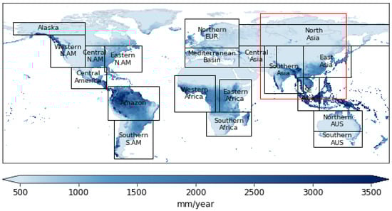
Figure 1.
Regional grid scale annual average precipitation (1901–2013) (precipitation data from [22]; regions defined in [23]). (Abbreviations: N., North; S., South; SE, Southeast, AM, America; AUS, Australia; EUR, Europe). A large Asian region box is superimposed (in red).
The regions outlined in black in Figure 1 were used in previous analyses carried out by [24] and they were also used initially by the IPCC in AR3 and AR4. They were chosen based on the following criteria: (1) the sizes of the rectangular regions vary in the range of a few thousand to several thousand km in each direction; these were originally chosen to facilitate grid-based analyses of GCM outputs [24], which in our case facilitated the grid-based analysis of the scale dependence of LTP (consistent rules for averaging over irregular regions at increasing scales are messy to construct); (2) we wanted to cover all global land areas approximately with a manageable number of previously designated climatic regions of simple regular shape that facilitated the scale-dependent analyses of LTP and the Hurst coefficient.
Naturalised annual river flow data are needed to investigate the link between LTP in the annual flows of large rivers and the scale dependence of LTP in precipitation, as abstractions and river regulation can distort estimates of the Hurst coefficient. Long records of naturalised flow data have been published for very few large rivers; we needed continuous records dating from 1900 to maintain consistency with the precipitation analyses. The Colorado river gauged at Lees Ferry (area 290,000 km2) satisfied both these criteria; naturalised annual flow data were obtained from the US Bureau of Reclamation. Continuous annual flow data for the Mississippi at Keokuk (area 308,000 km2) were obtained from 1900 from the Global Runoff Data Centre (GRDC). The Mississippi flow data were not naturalized.
2.2. Estimation of the Hurst Coefficient H
The Hurst coefficient was estimated using aggregated variance plot analysis [16,25], which is based on a property of the change in the statistical characteristics of a Hurst –Kolmogorov (HK) process with respect to the time scale of averaging [25]. The summary here is taken from [16].
For an HK time series split into nonoverlapping blocks of size n, the relationship between block size n and the variance in the block mean (the time-averaged process) is given by
where is the block mean, H is the Hurst coefficient and c is a constant. Using a range of block sizes, a double log plot of the variance in the block mean against the block size is constructed, with the data points expected to fall along a line with negative slope 2H − 2. A slope of -1 indicates independence (white noise), with a long-range dependent HK process with different H values having shallower slopes.
It should be noted that the term ‘aggregated variance’ is a misnomer as it is not the variance that is aggregated but the time scale; for this reason, the term climacogram has been coined [26].
The H values were calculated using the aggvarFit function in the R package fArma [27]. The block sizes (denoted as m in fArma) used in the calculation of the slope were the set of integer values in the range 4 ≤ m ≤ 14. For the GPCC data set, the maximum value of 14 provides eight values for calculation of the variance at the largest block size. The slope was obtained from the least square fit of the logarithm of the block sample mean variances versus the logarithm of the block sizes.
The standard variance estimator used in the R package fArma has been shown to be biased [28], with the bias being a function of H. For H < 0.7, the downward bias is negligible, but it becomes more noticeable above H = 0.8. The main conclusions of the paper about the spatial scale dependence of H are not affected by the bias.
2.3. Cumulative departure from the mean (CDM) plots
Cumulative departure from the mean (CDM) plots are a useful diagnostic tool for differentiating time series with upward and downward fluctuations that can result in similar H estimates. They are used in analysing the spatial scale dependence of average regional precipitation [16]. The CDM is defined as
where CDMk is the CDM at time point k, 1 ≤ k ≤ n where n is the length of the time series and is the mean.
2.4. Spatial Scale Analysis of H for Average Regional Precipitation
Starting at the (0.5 × 0.5 degree) grid scale, and for increasing spatial scales, each region was partitioned into nonoverlapping tiles using a moving window approach. Starting at the northwest corner of the region, the window was moved in an easterly direction by a distance equal to the width of the window, with the average precipitation calculated for each window position. On completion of the row, the window was moved in a southerly direction, by a distance equal to the window width, and the process repeated. Each window must lie entirely within the region. The Hurst coefficient was estimated for the average precipitation for each tile (in calculating the regional average precipitation values, the grid scale values were weighted by their projected earth surface areas) [16]. A box plot is used to display the sample frequency distribution of H against increasing scale.
2.5. Theoretical Explanation of the Increase in H with the Scale of Averaging
2.5.1. Introduction
The increase in H with the spatial scale of averaging found by [16] raises the question of how this might be explained theoretically. Here, a theoretical development is presented for the case of the sum (or weighted average) of two (or many) HK stochastic processes over time or space.
For a stationary stochastic process , where t denotes time and an underlined symbol denotes a stochastic (random) variable (the Dutch convention) and a nonunderlined symbol denotes a common variable, the Hurst parameter H is formally defined through the asymptotic relationship
where is a positive constant, H is the Hurst coefficient and is the climacogram, i.e., the variance of the averaged process at time scale , that is,
Now we consider the sum of two processes with climacograms and Hurst parameters , correlated with each other with (lag-zero) correlation at scale equal to . We denote and the climacogram and the Hurst parameter of the sum, respectively.
The following relationships, in which for notational brevity we have omitted , hold true always
For sufficiently large , the following approximations will be valid, becoming exact as .
for some . Hence
2.5.2. Components with Equal Hurst Parameter
Solving Equation (7) for we find
Assuming , this becomes
We wish to find . If , then
On the other hand, as it should hold that , this is only possible when and in this case . Any other case () would violate . This is a quite restrictive case not met in general.
If , then
which violates .
Thus, the only feasible case is , in which
Note, this is constant for all time scales for which the variances can be expressed as power laws of the time scales , and could be positive, negative or zero.
2.5.3. Components with Unequal Hurst Parameter
Now we assume From Equation (7), we obtain
Since
Hence
This means that the Hurst parameter of the sum of the two processes will be , i.e., equal to the maximum of the Hurst parameters of the two processes. Symbolically,
2.5.4. Generalization
Likewise, by induction, if we consider the sum of processes , then the Hurst parameter of the sum will be
Furthermore, since the Hurst parameter of a process does not change if we multiply the process by any constant, Equation (17) should also hold true if, instead of the sum of the processes , we take their weighted average, with arbitrary weights.
2.6. Crossing Properties of Regional Precipitation Deficits
As discussed in the Introduction, LTP influences the characteristics of precipitation deficits. The finding that LTP is enhanced and can be much stronger at the regional scale than evidenced by point precipitation analyses has implications for characterizing regional precipitation deficits. The crossing properties of a time series [29] are a useful basis for assessing the statistics of excursions above or below any predefined level of a time series. Here we investigate the crossing properties of precipitation deficits defined for the average regional precipitation time series Xt for each of the eight LTP regions identified by [16] and the period 1901–2013, and how well they can be described by the value of the Hurst coefficient H.
Figure 2 is used to define the crossing properties investigated. The duration D of a crossing below a predefined level is defined as the length of an excursion of annual average regional precipitation below the selected level. The volume V is the shaded area below the selected level, and for the annual time series analysed here, is assigned to the year in which the deficit ends. In what follows, this will be referred to as a volume deficit. A third measure employed is the intensity I, defined as V/D, which is assigned to the same year as V. Two crossing levels are used: (a) the mean and (b) the mean minus one standard deviation (MSD) of the average precipitation time series.
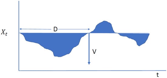
Figure 2.
Schematic of crossing properties.
If represents a member of a set of m deficits defined for each crossing level of the annual time series of length n years, then the average duration is defined as
To allow comparisons across the eight regions, the volumes are divided by the mean of the time series and converted to a percentage to give a standardised percentage volume
The average percentage volume is defined as
and the average intensity as
3. Results
3.1. Monte Carlo Simulation of Theoretical Scale Dependence of H
As the theoretical result (17) may appear counterintuitive, Figure 3 provides an intuitive explanation for the reasons it is actually valid and, at the same time, a confirmation using Monte Carlo simulation. The simulation was made by the method described in [30]. Time series of length 1000 were generated from HK processes independently from each other (), and the sum was defined as . The process has a large Hurst parameter, , while the process has a small one . However, at scale 1, the process has five times larger variance than that of (5 against 1, respectively) and times higher mean (22.4 against 10, respectively). However, because of the different H values, the variances of the two processes become equal at a time scale between 22 and 23, and beyond that the variance of the process , which initially was a small portion (1/6) of that of the process , dominates. This is illustrated in the slopes of the climacograms of Figure 3 (slope = 2H − 2), empirically estimated for scales . The slope for the time series generated from is −0.37 (theoretical value −0.4: H = 0.8) and that of is −0.97 (theoretical value ). The climacogram of the sum has slope −0.49, i.e., approaching the theoretical value of . Had the time series been longer, so that estimation of even larger time scales would be possible, the slope for the sum would tend to −0.4 (H = 0.8), i.e., H for the process is as predicted by (17).
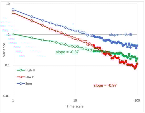
Figure 3.
Monte Carlo simulation of the scale dependence of H for the sum of two HK processes with different H parameters.
3.2. Spatial Scale Dependence of H for Average Annual Precipitation
In a previous work [16], 8 of the 19 regions outlined in black in Figure 1 were selected on the basis of having H > 0.6 for average grid-scale precipitation, and analysed for scale dependence of H. The mean value of H at the grid scale was 0.66 and, at the regional scale, 0.83, showing substantial enhancement at the latter scale. It was also shown that the increase in H with scale was linked to modes of long-term climatic variability, such as the AMO, the PDO and the IPO. It is possible that small-scale climatic variability/noise disguises the LTP signal at the point/grid scale, which emerges as the scale of averaging increases. Here, the scale dependence of H for the remaining 11 regions with grid scale H < 0.6 has been analysed
Box plots of H against the scale of averaging for the 11 regions are presented in Figure 4, and the results are summarized in Table 1. Central North America, Western North America and Southern Africa show a substantial increase in H at the regional scale, Central America and the Mediterranean Basin less so, and the remaining regions show no increase with scale, or a slight decrease. These latter regions all have weak LTP, with the exception of Alaska, which has H = 0.65 at the grid scale and H = 0.66 at the regional scale, i.e., moderate LTP (Alaska was omitted from the original set having grid scale H > 0.6 (16) because it exhibited no increase with scale). Overall, the mean value of H across the regions shows only a slight increase in H from the grid to the regional scale.
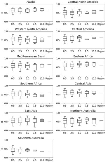
Figure 4.
Box plots showing scale dependence of H for the 11 selected regions. Units for x-axis are decimal degrees.

Table 1.
H values for the eleven selected regions at grid and regional scales.
ENSO has a dominant role within the global climate system, particularly in the Southern Hemisphere, and the Hurst behaviour it can induce in annual precipitation, as seen in the H values for Northern and Southern Australia in Table 1, merits a specific comment. ENSO is characterised by alternating El Nino and La Nina phases of random durations of 2–4 years, which can result in anti-persistence, or short-term, high-frequency fluctuations in annual precipitation, for which H < 0.5. However, this can mask underlying LTP, which can emerge at longer time scales. This is illustrated in the climacogram in Figure 5 for the average precipitation over Australia where, for short time scales, H = 0.3, while for longer time scales, H = 0.7, reflecting LTP induced by longer-term modes of oscillation such as the PDO.

Figure 5.
Climacogram separating short and long time scales for average precipitation over Australia (GPCC Version 2022 data set). The fitted linear relationship for the short time scales gives H = 0.30, reflecting the influence of ENSO, which is anti-persistent, while for the longer time scales, H = 0.71, reflecting LTP.
For the red box encompassing most of the Asian continent in the Northern Hemisphere in Figure 1, H has been calculated for a range of increasing scales of averaging, starting with the 0.5 × 0.5 degree grid scale (Figure 6). The results illustrate that H increases with scale up to the 40 decimal degree (40dd) scale of averaging (from 0.69 to 0.93), but then collapses to a value of 0.63 at the full regional scale. This surprising result may appear to be at variance with Equation (17) but it is not, as the latter is an asymptotic result. The sample time series data, which are observed at the 40dd scale, all have high H values (Figure 6) but distinctly different CDM plots (Figure 7) that reflect contrasting long-term modes of climatic fluctuation for the tropics and northern regions over the period of record. These tend to cancel each other out at the regional scale of averaging, even though the three 40dd boxes all have high H values.
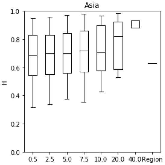
Figure 6.
Box plot showing scale dependence of H for the Asian region. Units for x-axis are decimal degrees.
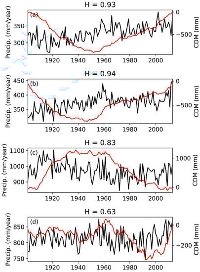
Figure 7.
Time series and CDM plots for the three 40dd boxes (a–c), and the full Asian region (d).
3.3. LTP in Catchment Boundary Box Precipitation and Rivers Flows
LTP in the annual flows of the river Nile at Aswan has been shown to be attributable to LTP in basin scale precipitation for the Blue Nile [16]. Here, we present results for two other large river basins: the Colorado at Lees Ferry, and the Mississippi at Keokuk.
Figure 8c,d show scale-dependent analyses of precipitation for rectangles bounding the Colorado and Mississippi catchment areas (a,b). There is a slight increase in H with scale for the Colorado (0.53 to 0.59), and a modest increase for the Mississippi (0.61 to 0.72). Time series and CDM plots for both rivers are presented in Figure 9 for both annual average precipitation and flows.
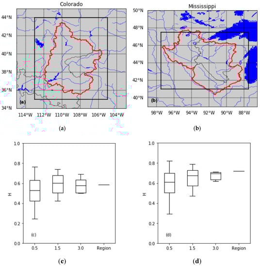
Figure 8.
(a,b) Catchment boundary boxes; (c,d) scale-dependent box plots of H for average annual precipitation for the Colorado at Lees Ferry (1906–2013) and the Mississippi at Keokuk (1901–2013).
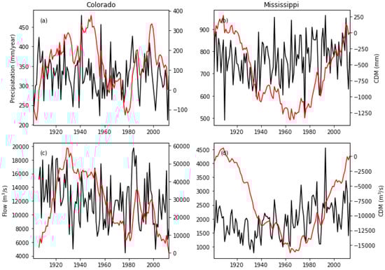
Figure 9.
Time series and CDM plots for average annual precipitation and annual flows for the Colorado at Lees Ferry (1906–2013) (a,c) and the Mississippi at Keokuk (1901–2013) (b,d).
Estimates of H are presented in Table 2 for the annual average catchment precipitation and annual flows for the Colorado and Mississippi rivers. For the Colorado, there is weak LTP in basin precipitation (Table 2: H = 0.59), reflecting the reversals in fluctuations seen in the CDM plot (Figure 9). However, the fluctuations seen in the CDM plot for annual precipitation in the later decades of the record are damped in the CDM plot for annual flows, indicating that the latter have been declining in this period, resulting in a higher H value for the flows of 0.69. This decline has been mainly attributed to increased evapotranspiration caused by a reduction in albedo from snow loss and the associated rise in the absorption of solar radiation [31]. Otherwise, the CDM plot shows that there is coherence between the longer-term fluctuations in annual flows and those in precipitation.
Table 2.
H estimates for catchment boundary box average annual precipitation (P) and annual flows (Q) for the Colorado river at Lees Ferry (1906–2013) and the Mississippi at Keokuk (1901–2013).
For the Mississippi, the fluctuations in the CDM plot for the annual flows at Keokuk clearly follow those for annual average precipitation, but the Hurst coefficient for the annual flows Q is higher (H = 0.84) than for precipitation P (H = 0.73) (Table 2). It is evident from Figure 9 that the annual flows are smoother than annual precipitation, most probably reflecting a degree of regulation, e.g., the low precipitation years are much less evident in the flows. The precipitation is therefore more ‘noisy’ than flow, which accounts for the lower H value. However, the CDM plot clearly shows that the long-term fluctuations in flow are coherent with those in precipitation.
3.4. Analysis of the Crossing Properties of Precipitation Deficits
Figure 10 presents plots of precipitation deficits for the eight regions for the period 1901–2013. Deficit periods of 5 years or more below the mean, with standardised volumes and intensities, are summarised in Table 3, together with embedded crossings below the MSD level. The threshold of 5 years is chosen to capture the longer deficits associated with LTP, and to keep the information in Table 3 manageable.
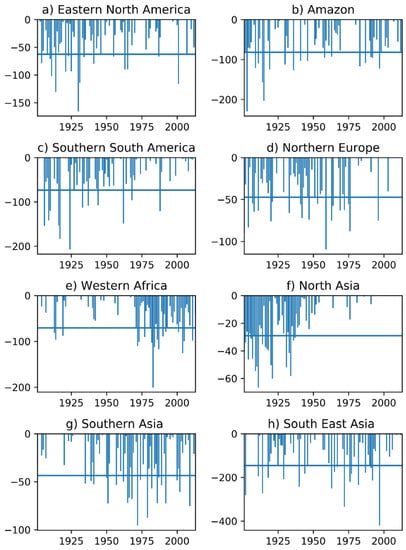
Figure 10.
Area average precipitation deficits below the mean and the MSD for the eight LTP regions, 1901–2013. Standard deviations are shown as horizontal lines. Units are mm.
Table 3.
Deficit periods (D) of more than 5 years below the mean, with percentage volumes (SV) and intensities (I), for average area precipitation for the 8 LTP regions for the period 1901–2013. Embedded deficits below MSD, with percentage volumes and intensities, are also shown.
Eastern North America (ENA), Amazon (AMZ) and Southern South America (SSA) show some regional coherence, in that the deficits occur predominantly in the early part of the twentieth century, although the timings of the deficits are different. ENA had three multi-year deficit periods below the mean (1907–11;1913–19 and 1921–27), with shorter embedded crossings of the MSD level. The volume percentages SV range from 27 to 32% of the mean range, while the MSD deficits range from 0.4 to 6%. The intensity range is 4–5% for the mean level, and 0.4–6% for the MSD level.
For Amazon and the mean level, there is an early 20th century deficit period of 6 years (1901–06), and a later deficit period of 5 years (1965–69), with volume deficits of 32.3% and 10.4%, and intensities of 5.4 and 2.1%, respectively. There is only one MSD deficit, which is for the early period, with volume and intensity of 8.2% and 2.7%, respectively. Southern South America has a five year deficit period in 1906–10, with volume and intensity of 57.2% and 11.4%, and two MSD crossings with volumes of 8.9% and 12.8%, respectively, and intensities of 8.9 and 6.4%. There are two further deficit periods in 1947–52 and 1967–71, with volumes of 27.0% and 26.2% and intensities of 4.5 and 5.2%, respectively. The former period has no MSD crossing, while the latter has one crossing with volume and intensity of 2.5% and 2.5%, respectively.
Northern Europe also has an early 20th century deficit period (1917–21) and an extended period of 12 years (1936–47), with volumes of 32.2% and 58.9%, and intensities of 6.4% and 4.9%, respectively. There are three short MSD crossings with volumes in the range 3.7–4.8% and intensities in the range 2.4–3.7%.
Western Africa stands out as a region with prolonged and intense deficits in the late 20th and early 21st centuries of 18 years (1970–87) and 12 years (2000–2011), respectively; these have volume deficits of 142.3% and 77.5% and intensities of 7.9 and 6.5%, respectively. These are interspersed with a five-year deficit period (1989–93) with volume and intensity of 34.8% and 7.0%, respectively. The major deficit periods are known to have had large socio-economic impacts, e.g., in the Sahel. There are several short embedded 1–3-year MSD deficit periods.
North Asia has extended deficit periods of 21 years (1901–21) and 18 years (1928–45) in the early part of the 20th century, and no later deficits, reflecting an almost continuous upward fluctuation over the period of record; the corresponding volume deficits and intensities below the mean are 184.4% and 8.8%, and 95.7% and 5.3%, respectively. There are multiple embedded MSD crossings of 1–3-year durations. In contrast, Southern Asia has a predominance of crossings in the latter half of the record, with two deficit periods of 8 years (1962–69) and 5 years (2000–04); they have volumes of 42.8% and 22.2%, and intensities of 5.4 and 4.4%. These two deficit periods have five 1–2-year MSD crossings, with a volume percentage range of 0.8–6.6%, and an intensity range of 0.8–6.3%. Southeast Asia also has a greater number of crossings in the second half of the record, with two deficit periods of six years in 1925–30 and 1989–94; these have percentage volumes below the mean of 23.4% and 30.7%, and intensities of 3.9% and 5.1%, respectively. There are three 1–3-year MSD deficits, with volume and intensity ranges of 0.1–3.4% and 0.1–2.5%, respectively.
These results are summarised in Table 4 by the means of the three crossing measures for the two crossing levels, with the means, standard deviations, coefficients of variation and Hurst coefficients of the regional time series also shown. North Asia and West Africa have the longest average durations below the mean and MSD, with correspondingly high percentage volume deficits below the mean and MSD; these results are consistent with the high H values for these regions.
Table 4.
Summary statistics and average crossing properties for areal average precipitation below the mean and MSD for the 8 regions for the period 1901–2013.
In Figure 11, plots of , and against the Hurst coefficient H (Table 4) are presented for the mean crossing level ((a)–(c)) and the MSD crossing level ((d)–(f)). For the former case, there is a strong correlation between both and H and and H, which is less well defined for the MSD crossing due to the smaller number of deficits below this level. There is no evident correlation between and H. West Africa (H = 0.91) and North Asia (0.99) have the highest H values, and the longest duration deficit periods and volume percentages among the set of eight regions. H is evidently a good descriptor of the susceptibility of the eight regions to persistent precipitation deficits.

Figure 11.
Plots of , and against H for the mean crossing level (a–c) and the MSD level (d–f).
Regional averages of duration and volume percentage , taken across the eight regions for the two crossing levels, and the period of record 1901–2013, are presented in Figure 12. To allow the multi-decadal variability of , and to be assessed, grand averages across regions and years have been computed for three periods:
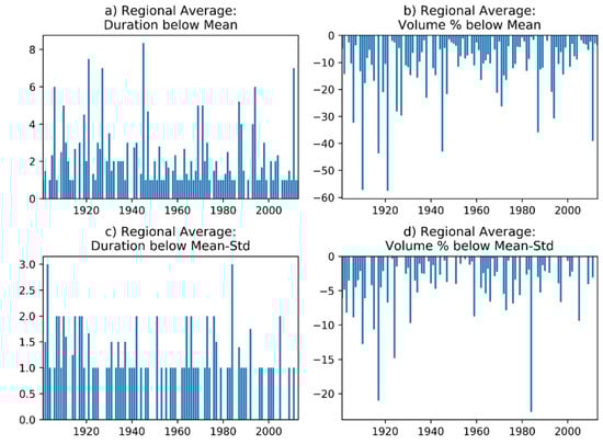
Figure 12.
Regional averages of deficit duration and volume percentage for each year for the mean and MSD crossing levels, 1901–2013.
- Period 1: 1901–1938 (38 years)
- Period 2: 1939–1976 (38 years)
- Period 3: 1977–2013 (37 years)
In particular, this allows evidence for any anthropogenic climate change (ACC) signal in Period 3 to be assessed. The results for the three periods are summarised in Table 5(i) and Figure 13(i). No evidence of ACC intensification is apparent for Period 3.
Table 5.
Grand averages of the crossing statistics , and taken across the 8 regions and years for the mean and MSD crossing levels and Periods 1–3. The proportion of years in which no crossing event occurred across the set of regions is also shown.
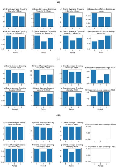
Figure 13.
Plots of grand averages of the crossing statistics , and taken across regions and Periods 1–3 for the mean crossing level (a–c) and MSD level (e–g). The proportion of years in which no crossing event occurred across the set of regions is also shown (d,h). (i) For the 8 LTP regions and the 1900–2013 data set; (ii) for the 8 LTP regions and the extended 1900–2020 dataset; (iii) for all 19 regions and the extended 1900–2020 data set. (Note, different vertical scales.)
To explore the effect of more recent data on our results, the 1901–-2013 data set was extended up to and including 2020 using the GPCC 2022 data set (which, despite its label, only includes data up to 2020). Firstly, the eight LTP regions were analysed, and there is no evidence of any enhancement of precipitation deficits in the last period (3 periods of 40 years were used) (Table 5(ii) and Figure 13(ii)). Finally, all 19 regions were analysed using the extended data set, and the results show that some of the sampling variability in the results for the eight regions was averaged out, with no apparent ACC deficit intensification evident in the last period. Crossings occurred in every year for both levels (Table 5(iii) and Figure 13(iii)).
4. Discussion
In what follows, we discuss the specific results reported above, and then broaden the discussion to express some views and opinions on related hydrology and water resources issues, and on how the findings presented here and in previous papers we have published might inform sustainable water resources policy making, particularly for risk assessments.
4.1. Spatial Scale Dependence of H For Annual Average Precipitation
Firstly, the results we obtained are a function of the regions chosen, their scale and shape, and we justified our choice of these in Section 2.1 above. Sensitivity to these factors might be explored in further work, but based on the results in (16) and those presented here, we are confident on the validity of our main findings on the scale dependence of LTP and H.
The results for the 11 regions show that Central North America, Western North America and Southern Africa have a substantial increase in H at the regional scale, Central America and the Mediterranean Basin less so, and the remaining regions show no increase, or a slight decrease with scale. These latter regions all have weak LTP, with the exception of Alaska, which has H = 0.65 at the grid scale and H = 0.66 at the regional scale, i.e., moderate LTP but with no scale dependence.
There is an apparent inconsistency between the theoretical explanation of the asymptotic increase in H with the scale of averaging (17), confirmed by Monte Carlo simulation, and the sample result obtained for the Asian region (Section 3.2) where H has decreased at the full regional scale. The latter result can be viewed as a statistical artefact in the context of the theory, and can be explained as follows. At the 40dd scale of averaging, there are three boxes that are averaged to give the regional scale result (Figure 7):
- Western Russia, with an H of 0.93
- Eastern Russia, with an H of 0.94
- India and the Himalayas, with an H of 0.83.
According to the theoretical result (17), H for the Asian regional scale should be 0.94, but the opposite mode of climatic fluctuation observed in the CDM plot (Figure 7) for subregion 3 results in the decrease in H at the full Asian region scale to H = 0.63. Sample estimates of H cannot distinguish between a predominantly upward fluctuation and a predominantly downward fluctuation. These opposing fluctuations are averaged out asymptotically in an HK process so there is no inconsistency with the theory.
The areas of the eight strong LTP regions from Figure 1 analysed for H scale dependence in [16] (land area range 2.4–14.7 × ) are of the same order of magnitude of those of the three 40dd regions 1–3 analysed here (area range 8.8–10.0 ), and all eight exhibited no reduction in H at a full regional scale, so it seems that the spheres of influence of the relevant modes of climatic fluctuation are at least as large as these scales but lessen as the scale of averaging increases to include other opposing modes of oscillation. There is an extensive literature on the NAO, AMO, IPO, PDO, etc., influences on regional and global precipitation, which would need to be analysed to define their spheres of influence; these might be made up of land areas that are not contiguous. This is outside the scope of this paper.
4.2. Consistency of LTP in Annual Flows with Ltp in Basin Average Precipitation
The results obtained for the Colorado and Mississippi rivers in Section 3.3 show that the long-term fluctuations in annual flows are driven predominantly by those in basin average rainfall. The enhancement of H for the naturalised Colorado flows over that for rainfall is apparently due to the decline in flows, which has been attributed to the enhancement of evaporation associated with a declining snowpack [31]. For the Mississippi, the enhancement can be attributed to the effects of regulation as the flows are not naturalised. Similar analyses of other large rivers are restricted by the record lengths available (estimates of H need to be based on record lengths comparable to precipitation, and they become too variable if short record lengths are used (100 years is still short in the presence of LTP as the information content is low).
To investigate how the scale dependence of LTP in large basin average rainfall translates into LTP in river flows, a distributed monthly rainfall–runoff modelling approach could be adopted using GPCC gridded monthly rainfall. This would allow the effects of regulation and other factors that create trends in flows to be isolated from the effects of LTP, enhancing attribution.
4.3. Characteristics Of Precipitation Deficits For The Eight Ltp Regions
The analysis of the crossing properties of average regional precipitation deficits using the 1900–2013 data set shows that some regions encountered deficits predominantly in the early part of the 20th century, while other regions were in surplus over the same period. The averages of the D, SV and I statistics across the eight regions for each year suggest that there is a levelling up of the crossings between the first and second half of the record (Figure 12), and with relatively low volumes in the middle period. The grand averages for Periods 1–3 (Table 5(i) and Figure 13(i)) do not suggest that there is any intensification of precipitation deficits in Period 3 that might be attributed to ACC. On the contrary, the statistics suggest that Period 1 is characterised by more severe deficits, with the lowest deficits and intensities below the MSD level in Period 2. It also appears that the proportion of years in which no crossing of the MSD level occurs is increasing, indicating that fewer crossings of this level are occurring, but these results have high uncertainty due to the small number of crossings. Significance tests on the differences between the proportions requires the assumption of independence, which is unlikely to be satisfied in this case.
The results obtained using GPCC data up to and including 2020 for the eight LTP regions (Table 5(ii) and Figure 13(ii)) do not suggest that there is any signal emerging in recent data that could be attributed to the intensification of precipitation deficits from ACC. This is also the case for all 19 regions analysed using data up to 2020 (Table 5(iii) and Figure 13(iii)).
4.4. Precipitation Deficits, Droughts And Anthropogenic Climate Change
In analysing the evidence for any recent global warming influence on precipitation deficits, the IPCC [32] noted that, while some regions of the world had recorded strong precipitation deficits in recent decades, other regions had not. They noted that global studies had generally shown no significant trends in SPI time series, and in derived drought frequency and severity data, and concluded that natural climatic variability is still the dominant mode of variability governing precipitation deficits and droughts, and, by implication, LTP. This conclusion is supported by our findings here, where we have not seen any clear evidence of intensification in precipitation data up to and including 2020 (Table 5 and Figure 13). Moreover, the narrative on causality continues to evolve [33,34,35,36].
Droughts are increasingly governed by a complex mix of physical and socio-economic factors. However, the overarching global concern about anthropogenic climate change (ACC) frequently results in droughts being at least partly attributed to ACC. However, given our findings about LTP and high natural variability, the main physical risk of precipitation deficits is coming from LTP. Many governments include water resources planning and management under the umbrella of their ACC mitigation and adaptation policies, with major reliance placed on GCM projections. Successive generations of GCMs have been shown to be deficient in reproducing natural climatic variability [37,38,39,40,41]. A recent study [39] revealed systematic errors in the representation of drought persistence in the then current GCMs. The newer model generations continue to exhibit this deficiency; output data from the Coupled Model Intercomparison Project (CMIP6) was recently found to be inconsistent with reality for the entire region of Italy [42].
The reliance on GCM projections in adaptation planning can place undue emphasis on an expected outcome. For example, several climate models projected an increase in precipitation in East Africa in future decades, whereas some severe droughts materialised [18]; this has implications for developing viable adaptation policies. However, multiple factors are deemed to be at play in what has come to be known as the East African Paradox, and a conclusive explanation for this has yet to emerge [18]. Nonetheless, this outcome does demonstrate that adaptation planning based on one expected scenario may not be robust under other scenarios and high uncertainty. Adaptation plans need to be tested against an envelope of uncertainty for future precipitation. It is relevant to mention here the prolonged (7-year) drought that occurred in Greece around 1990, which severely affected the water supply system of Athens. The management of the situation was quite effective as it was based on an HK stochastic framework [9].
Recent droughts are being reported in many regions of the world, and water crises are also being reported. While the results presented here would suggest that many of these droughts that result primarily from precipitation deficits can be a consequence of natural climatic variability, it is the case that many are attributed a priori to nonstationarity caused by ACC, supported by trend analysis, the Mann–Kendall test, etc. Scientific investigations frequently start from the premise that ACC is an explanatory factor, and set out to prove it, whereas a more conventional scientific approach would be to adopt the Null Hypothesis that natural climatic variability is a causal factor, and to test the Alternative Hypothesis that it is ACC. In this regard, the use and misuse of trend tests, and the misunderstanding of stationarity have been analysed and discussed in a number of papers (e.g., [43,44,45,46]), and it is good to see that more considered approaches are now emerging in the literature (e.g., [47,48,49]). That ACC can be a factor influencing droughts is not in question, but based on current evidence, natural climatic variability remains the main driver of precipitation deficits in regions affected by LTP, but care is needed that apparent trends resulting from LTP are not misinterpreted as evidence of ACC.
Stochastic HK simulations reproducing the Hurst coefficient can capture the full envelope of uncertainty resulting from LTP for a risk assessment of annual precipitation deficits [50] rather than approaches that focus on weak dependencies on climatic modes of variability such as the NAO, e.g., [19], which may not capture LTP adequately. The NAO does not affect total annual precipitation but influences its spatial and seasonal distribution [51]. No significant correlation was found between average annual regional precipitation and the NAO for the eight LTP regions listed in Table 4 [16].
4.5. Implications For Policy Making And Risk Assessment In Sustainable Water Resources Planning And Management
The climate has always been naturally variable, and the key manifestation of this variability in the fields of hydrology and water resources management is in precipitation. Our recent findings show that precipitation, when averaged over increasing spatial scales, is much more naturally variable than we would think based on the analysis of point precipitation. This explains why the annual flows of some large rivers such as the Nile exhibit much more variability/LTP than point precipitation would reveal, and precipitation deficits at a regional scale will therefore be more severe. This has implications for drought adaptation planning in vulnerable regions of the world such as East Africa, and for water resources management, both surface and subsurface. Major aquifers are recharged over large areas, so will be affected by area average LTP. The Hurst coefficient is the key parameter in describing this, and in undertaking risk analyses.
In determining the yields of reservoirs and river abstractions, the average flow over the available period of record is the key quantity used to determine the yield that can be maintained as a proportion of the mean flow. The reliability of the yield is usually assessed by running a simulation over the period of record. However, in the presence of LTP, the mean flow is highly variable, and its increase with H is described by (1). As a consequence, the information content of a record reduces sharply [9], and the typical record lengths available are woefully inadequate for estimating yield reliably in the presence of LTP. This can have some unintended consequences. Suppose the record covers a period of above average long-term flows, and a period of below average flows is subsequently encountered during operation, there will be adverse impacts on water supplies, and the projected benefits of the investment will not be realised. If the design is based on a below average period of flows, and a period of above average flows follows, all is fine, but there will be the temptation to use the surplus water rather than let it go to sea when the demand is growing. This makes yields more vulnerable to future reversals in flow resulting from precipitation deficits and droughts. The climate has always had the capacity to surprise, particularly in the presence of LTP. This is basic hydrological understanding that, in current times, is lost sight of in the quest to attribute droughts and water crises to anthropogenic climate change (ACC). This does not necessarily mean that ACC is not a factor, and it is expected that it might enhance/intensify LTP in the future, but the strength of the underlying LTP will be the dominant factor in determining the severity of precipitation deficits. Risk analyses based on HK simulations should explore the sensitivity to an increase in H to reflect ACC intensification.
Most governments nowadays have policies aimed at reducing emissions and planning adaptation to ACC that reach across all sectors, including water. GCM projections and related products (e.g., downscaled precipitation generators) are prescribed as mandatory for adaptation planning. However, as noted above, GCMs still do not reproduce the persistence that generates multi-year droughts, and so drought risks will be underestimated for those regions affected by LTP. The essentially deterministic nature of GCM projections (e.g., precipitation in a region is expected to increase over the coming decades) is also a problem as the full uncertainty in these projections is not captured by ensembles, but recent developments by hydrologists demonstrate how the uncertainty in these conditional projections can be better represented [42,52]. It is relevant to note that, according to the analysis by [34], even when accepting the IPCC assertions, the changes in precipitation are a priori framed in the range of 1% to 3% per °C. In hydrology, such percentages are negligible compared to the natural variability (particularly in view of the Hurst behaviour), and even to the uncertainty in the measurement of precipitation. It is thus puzzling why hydrologists have followed such nonsensical mandates and continue to consider future projections of climate models for adaptation planning.
Accelerating socio-economic growth and demand for water in many countries across the globe has led to the depletion of water resources [53]. Gaps between supply and demand are developing, leading to water crises, and some countries are likely to run out of water by 2030 [54]. Those regions and countries affected by LTP will be more at risk and vulnerable due to more severe precipitation deficits. Despite the best efforts of UN Water to encourage the implementation of Integrated Water Resources Management (IWRM) through its numerous WWDR reports, sustainable development has demonstrably not been implemented. Concerned by this situation, and reflecting the concern of the World Economic Forum about the threat to the global economy posed by water crises, and to their own businesses, a group of banks and multi-nationals created the 2030 Water Resources Group (2030WRG) and published a report in 2009 that set out how country gaps between supply and demand could be closed by 2030. This could be achieved by focusing on demand management and improved water use efficiency, which have to be central to sustainable water resources management. They demonstrated, through economic analyses of water use efficiency opportunities for a number of countries, that their water gaps could be closed at much less cost than the conventional approach of supply-side investment, which has increasingly failed to respect the needs of the water environment. Moreover, under high levels of uncertainty, large supply-side capital investments should be avoided, and incremental investments based on water use efficiency preferred that are essentially ‘no regret’, i.e., they should be made in any case from a sustainability perspective [53]. This will require major shifts in water use behaviour, just as major behavioural shifts are required to reduce emissions. Whatever the future impacts of ACC (and the 2030WRG did not include ACC in their analyses), water crises are happening now, and the necessary investments in the water sector are needed to achieve a paradigm shift towards sustainable water use. The 2030WRG has been absorbed into the World Bank Group, and, to date, has formed 1009 public–private–civil society partnerships in 14 countries to deliver USD 993 M of investment in support of ‘collective action on water security for people, environment and economy’ [55].
Thus, why has it fallen to the private sector to take the lead in demonstrating how a sustainable approach to water resources management can be achieved? Multi-nationals are known for preparing business plans that look 20 years ahead, and this is rarely the case for public sector bodies. It can also be argued that the ability to leverage private sector funding is a significant advantage, as well as a culture of hitting targets within prescribed time scales. Despite the huge effort made by UN Water to mobilise the implementation of IWRM through the Sustainable Development Goals and its many reports, its uptake has been far too slow.
Thus, what are the implications for policy making in the field of water resources management? In many countries, water is not included in national economic planning, and the water sector is expected to meet the needs of other sectors primarily through a supply-side approach, i.e., deliver the water that is needed by whatever means to support the economic growth imperative. Globalisation has added to the pressure to deliver the necessary water. Resource depletion inevitably follows, and countries that are affected by LTP in precipitation will be much more at risk of developing water crises. They need to be made aware of this, and, based on the results presented here on precipitation deficits where no ACC signal is evident, to realise that ACC is not the main threat that they are at risk from. Policy making should integrate risk assessment of the impacts of LTP into sustainable water resources planning and management for those countries where LTP can be shown to be a threat.
The GPCC data set, which now includes data up to and including 2020, is a good starting point for doing a baseline assessment of the risk of precipitation deficits arising from LTP for a river basin. A more complete risk assessment would require the estimation of H to enable HK stochastic simulations of basin precipitation that can be fed into a monthly rainfall–runoff model to ‘stress-test’ the water resource system [56], as used originally within the Harvard Water Programme [57]. All of this would need to be packaged and made available for use by practitioners in a form that would enhance its use to test the robustness and resilience of water resources plans alongside the use of GCM projections. This would allow any deficiencies in the latter to be identified. Globally, the mainstream focus of global water resources planning and management should place more emphasis on adaptation to the population growth and socio-economic changes that are happening now and that will continue to happen in the coming decades. There needs to be a greater focus on investment options that will be robust and resilient to the risks to stressed water resource systems from an ever-changing climate, and which embrace sustainability [53]. Otherwise, economic growth itself, and lifestyles and livelihoods, will be placed at risk, and the water environment will suffer even more damage.
5. Conclusions
The main conclusions that can be drawn from our findings are:
- A theoretical result was derived for an HK stochastic process that explains how the Hurst coefficient can increase with the spatial scale of averaging, as observed for regional annual precipitation.
- Analysis of 11 climatic regions that exhibit weak LTP at the grid scale (H < 0.6) showed that five of the regions exhibit an increase in H with the scale of averaging, while the remainder do not.
- For a large region of Asia, an increase in H was observed up to the full regional scale of averaging, but a decrease was observed at the full regional scale, which was shown to be a consequence of contrasting modes of climatic oscillation for the subregions averaged. This result can be viewed as a statistical artefact in relation to theory, which would disappear as the sample size became very large.
- For the Colorado and Mississippi basins, LTP in annual river flows was shown to be attributable to LTP in basin average precipitation.
- For average precipitation at the regional scale, the Hurst coefficient H was shown to be a good descriptor of the crossing properties of precipitation deficits below the mean and the mean minus one standard deviation, both in terms of duration and volume.
- From a multi-decadal analysis of the crossing properties, no evidence was found to show that there has been any increase in precipitation deficits in recent decades that might be attributable to global warming.
- Precipitation deficits are a consequence of natural climatic variability/the level of LTP, so the Hurst coefficient and HK stochastic simulations conditioned on a historic data set should be used to test water resource system resilience and robustness, and not rely exclusively on GCM projections that do not reproduce the LTP in observational records.
- To facilitate the assessment of risk arising from LTP by water resources managers, a package for risk assessment and resilience and robustness testing should be developed and made available on the web in a form that will facilitate uptake.
In addition to that specified in (8) above, future work could explore the sensitivity of the scale dependence of precipitation to region choice, scale and shape. Mapping the zones of influence of the major modes of climatic variability affecting LTP would provide an insight into regions where conflict between these modes leads to weak LTP. Monthly rainfall–runoff modelling of large river basins as a function of scale-dependent LTP in precipitation would enhance understanding of the evolution of LTP in river flows with increasing scale in these basins.
Author Contributions
Conceptualization, E.O.; methodology, all authors; software, G.O. and D.K.; formal analysis, all authors; writing—original draft preparation, E.O. and D.K.; writing—review and editing, all authors.; visualization, all authors. All authors have read and agreed to the published version of the manuscript.
Funding
Greg O’Donnell was supported by the Water Security and Sustainable Development Hub, funded by the UK Research and Innovation Global Challenges Research Fund (ES/S008179/1).
Data Availability Statement
The GPCC version 7 data set may be downloaded from: https://opendata.dwd.de/climate_environment/GPCC/html/fulldata_v7_doi_download.html (accessed on 29 June 2022). The GPCC Full Data Monthly Product Version 2022 is available from http://climexp.knmi.nl/select.cgi?id=someone@somewhere&field=gpcc_05 (accessed on 29 June 2022). Colorado at Lees Ferry data were downloaded from the Bureau of Reclamation site: https://www.usbr.gov/lc/region/g4000/NaturalFlow/provisional.html (accessed on 29 June 2022). Flow data for the Mississippi at Keokuk were obtained from the Global Runoff Data Centre (GRDC): https://www.bafg.de/GRDC/EN/02_srvcs/22_gslrs/221_MRB/riverbasins_node.html (accessed on 29 June 2022). The R package fArma may be obtained from https://github.com/cran/fArma (accessed on 29 June 2022).
Acknowledgments
We thank Alan Seed and three anonymous reviewers for their constructive comments that helped us improve the paper substantially.
Conflicts of Interest
The authors declare no conflict of interest.
References
- Hurst, H.E. Methods of using long-term storage in reservoirs. Proc. Inst. Civ. Eng. 1956, 5, 519–543. [Google Scholar] [CrossRef]
- Hurst, H.E. Long-Term Storage Capacity of Reservoirs. Trans. Am. Soc. Civ. Engineers 1951, 116, 770–799. [Google Scholar] [CrossRef]
- Mandelbrot, B.B.; Wallis, J.R. Noah, Joseph, and Operational Hydrology. Water Resour. Res. 1968, 4, 909–918. [Google Scholar] [CrossRef]
- Mandelbrot, B.B.; Wallis, J.R. Computer Experiments With Fractional Gaussian Noises: Part 1, Averages and Variances. Water Resour. Res. 1969, 5, 228–241. [Google Scholar] [CrossRef]
- O’Connell, P.E. Stochastic modelling of long-term persistence in streamflow sequences; Imperial College: London, UK, 1974. [Google Scholar]
- O’Connell, P. A simple stochastic modelling of Hurst’s law. In Proceedings of the International Symposium on Mathematical Models in Hydrology, Warsaw, Poland, 26–31 July 1974; pp. 169–187. [Google Scholar]
- Boes, D.C.; Salas, J.D. Nonstationarity of the mean and the hurst Phenomenon. Water Resour. Res. 1978, 14, 135–143. [Google Scholar] [CrossRef]
- Hosking, J.R.M. Modeling persistence in hydrological time series using fractional differencing. Water Resour. Res. 1984, 20, 1898–1908. [Google Scholar] [CrossRef]
- Koutsoyiannis, D. Hurst-Kolmogorov Dynamics and Uncertainty. J. Am. Water Resour. Assoc. 2011, 47, 481–495. [Google Scholar] [CrossRef]
- O’Connell, P.E.; Koutsoyiannis, D.; Lins, H.F.; Markonis, Y.; Montanari, A.; Cohn, T. The scientific legacy of Harold Edwin Hurst (1880–1978). Hydrol. Sci. J. 2016, 61, 1571–1590. [Google Scholar] [CrossRef]
- Markonis, Y.; Koutsoyiannis, D. Climatic Variability Over Time Scales Spanning Nine Orders of Magnitude: Connecting Milankovitch Cycles with Hurst–Kolmogorov Dynamics. Surv. Geophys. 2013, 34, 181–207. [Google Scholar] [CrossRef]
- Iliopoulou, T.; Papalexiou, S.M.; Markonis, Y.; Koutsoyiannis, D. Revisiting long-range dependence in annual precipitation. J. Hydrol. 2018, 556, 891–900. [Google Scholar] [CrossRef]
- Bunde, A.; Büntgen, U.; Ludescher, J.; Luterbacher, J.; von Storch, H. Is there memory in precipitation? Nat. Clim. Change 2013, 3, 174–175. [Google Scholar] [CrossRef]
- Mudelsee, M. Long memory of rivers from spatial aggregation. Water Resour. Res. 2007, 43. [Google Scholar] [CrossRef]
- Potter, K.W. Annual precipitation in the northeast United States: Long memory, short memory, or no memory? Water Resour. Res. 1979, 15, 340–346. [Google Scholar] [CrossRef]
- O’Connell, E.; O’Donnell, G.; Koutsoyiannis, D. On the spatial scale dependence of long-term persistence in global annual precipitation data and the Hurst Phenomenon. Water Resour. Res. 2022; in review. [Google Scholar]
- Camuffo, D.; Bertolin, C.; Diodato, N.; Cocheo, C.; Barriendos, M.; Dominguez-Castro, F.; Garnier, E.; Alcoforado, M.J.; Nunes, M.F. Western Mediterranean precipitation over the last 300 years from instrumental observations. Clim. Change 2013, 117, 85–101. [Google Scholar] [CrossRef]
- Rowell, D.P.; Booth, B.B.B.; Nicholson, S.E.; Good, P. Reconciling Past and Future Rainfall Trends over East Africa. J. Clim. 2015, 28, 9768–9788. [Google Scholar] [CrossRef]
- Gudmundsson, L.; Seneviratne, S.I. Anthropogenic climate change affects meteorological drought risk in Europe. Environ. Res. Lett. 2016, 11, 044005. [Google Scholar] [CrossRef]
- Cook, B.I.; Seager, R.; Williams, A.P.; Puma, M.J.; McDermid, S.; Kelley, M.; Nazarenko, L. Climate Change Amplification of Natural Drought Variability: The Historic Mid-Twentieth-Century North American Drought in a Warmer World. J. Clim. 2019, 32, 5417–5436. [Google Scholar] [CrossRef]
- Garreaud, R.D.; Boisier, J.P.; Rondanelli, R.; Montecinos, A.; Sepúlveda, H.H.; Veloso-Aguila, D. The Central Chile Mega Drought (2010–2018): A climate dynamics perspective. Int. J. Climatol. 2020, 40, 421–439. [Google Scholar] [CrossRef]
- Schneider, U.; Becker, A.; Finger, P.; Meyer-Christoffer, A.; Rudolf, B.; Ziese, M. GPCC Full Data Monthly Product Version 7.0 at 0.5: Monthly Land-Surface Precipitation from Rain-Gauges built on GTS-based and Historic Data. 2015. Available online: https://opendata.dwd.de/climate_environment/GPCC/html/fulldata_v7_doi_download.html (accessed on 2 November 2022).
- Harris, I.; Jones, P.D.; Osborn, T.J.; Lister, D.H. Updated high-resolution grids of monthly climatic observations—The CRU TS3.10 Dataset. Int. J. Climatol. 2014, 34, 623–642. [Google Scholar] [CrossRef]
- Giorgi, F.; Francisco, R. Uncertainties in regional climate change prediction: A regional analysis of ensemble simulations with the HADCM2 coupled AOGCM. Clim. Dyn. 2000, 16, 169–182. [Google Scholar] [CrossRef]
- Beran, J. Statistics for Long-Memory Processes; Routledge: London, UK, 1994. [Google Scholar]
- Koutsoyiannis, D. HESS Opinions "A random walk on water". Hydrol. Earth Syst. Sci. 2010, 14, 585–601. [Google Scholar] [CrossRef]
- Wuertz, D.; Setz, T.; Chalabi, Y. fArma: Rmetrics—Modelling ARMA Time Series Processes. R package, Version 3042.81. 2017. Available online: http://cran.nexr.com/web/packages/fArma/index.html (accessed on 2 November 2022).
- Tyralis, H.; Koutsoyiannis, D. Simultaneous estimation of the parameters of the Hurst–Kolmogorov stochastic process. Stoch. Environ. Res. Risk Assess. 2011, 25, 21–33. [Google Scholar] [CrossRef]
- Nordin, C.F.; Rosbjerg, D.M. Applications of crossing theory in hydrology. Int. Assoc. Sci. Hydrol. Bull. 1970, 15, 27–43. [Google Scholar] [CrossRef]
- Koutsoyiannis, D. Generic and parsimonious stochastic modelling for hydrology and beyond. Hydrol. Sci. J. 2016, 61, 225–244. [Google Scholar] [CrossRef]
- Milly, P.C.D.; Dunne, K.A. Colorado River flow dwindles as warming-driven loss of reflective snow energizes evaporation. Science 2020, 367, 1252–1255. [Google Scholar] [CrossRef]
- Seneviratne, S.I.; Zhang, X.; Adnan, M.; Badi, W.; Dereczynski, C.; Di Luca, A.; Ghosh, S.I.; Iskandar, J.; Kossin, S.; Lewis, F.; et al. Weather and Climate Extreme Events in a Changing Climate. In Climate Change 2021: The Physical Science Basis. Contribution of Working Group I to the Sixth Assessment Report of the Intergovernmental Panel on Climate Change, Section 11.6.1.1; Intergovernmental Panel on Climate Change: Geneva, Switzerland, 2021. [Google Scholar]
- Stephens, G.L.; Hakuba, M.Z.; Kato, S.; Gettelman, A.; Dufresne, J.-L.; Andrews, T.; Cole, J.N.S.; Willen, U.; Mauritsen, T. The changing nature of Earth’s reflected sunlight. Proc. R. Soc. A Math. Phys. Eng. Sci. 2022, 478, 20220053. [Google Scholar] [CrossRef]
- Koutsoyiannis, D. Revisiting the global hydrological cycle: Is it intensifying? Hydrol. Earth Syst. Sci. 2020, 24, 3899–3932. [Google Scholar] [CrossRef]
- Koutsoyiannis, D.; Onof, C.; Christofides, A.; Kundzewicz, Z.W. Revisiting causality using stochastics: 1. Theory. Proc. R. Soc. A Math. Phys. Eng. Sci. 2022, 478, 20210835. [Google Scholar] [CrossRef]
- Koutsoyiannis, D.; Onof, C.; Christofidis, A.; Kundzewicz, Z.W. Revisiting causality using stochastics: 2. Applications. Proc. R. Soc. A Math. Phys. Eng. Sci. 2022, 478, 20210836. [Google Scholar] [CrossRef]
- Johnson, F.; Westra, S.; Sharma, A.; Pitman, A.J. An Assessment of GCM Skill in Simulating Persistence across Multiple Time Scales. J. Clim. 2011, 24, 3609–3623. [Google Scholar] [CrossRef]
- Rocheta, E.; Sugiyanto, M.; Johnson, F.; Evans, J.; Sharma, A. How well do general circulation models represent low-frequency rainfall variability? Water Resour. Res. 2014, 50, 2108–2123. [Google Scholar] [CrossRef]
- Moon, H.; Gudmundsson, L.; Seneviratne, S.I. Drought Persistence Errors in Global Climate Models. J. Geophys. Res: Atmos. 2018, 123, 3483–3496. [Google Scholar] [CrossRef] [PubMed]
- Anagnostopoulos, G.G.; Koutsoyiannis, D.; Christofides, A.; Efstratiadis, A.; Mamassis, N. A comparison of local and aggregated climate model outputs with observed data. Hydrol. Sci. J. 2010, 55, 1094–1110. [Google Scholar] [CrossRef]
- Koutsoyiannis, D.; Efstratiadis, A.; Mamassis, N.; Christofides, A. On the credibility of climate predictions. Hydrol. Sci. J. 2008, 53, 671–684. [Google Scholar] [CrossRef]
- Koutsoyiannis, D.; Montanari, A. Climate Extrapolations in Hydrology: The Expanded Bluecat Methodology. Hydrology 2022, 9, 86. [Google Scholar] [CrossRef]
- Cohn, T.A.; Lins, H.F. Nature’s style: Naturally trendy. Geophys. Res. Lett. 2005, 32. [Google Scholar] [CrossRef]
- Clarke, R.T. On the (mis)use of statistical methods in hydro-climatological research. Hydrol. Sci. J. 2010, 55, 139–144. [Google Scholar] [CrossRef]
- Serinaldi, F.; Kilsby, C.G.; Lombardo, F. Untenable nonstationarity: An assessment of the fitness for purpose of trend tests in hydrology. Adv. Water Resour. 2018, 111, 132–155. [Google Scholar] [CrossRef]
- Koutsoyiannis, D. Climate change, the Hurst phenomenon, and hydrological statistics. Hydrol. Sci. J. 2003, 48, 3–24. [Google Scholar] [CrossRef]
- Merz, B.; Vorogushyn, S.; Uhlemann, S.; Delgado, J.; Hundecha, Y. HESS Opinions "More efforts and scientific rigour are needed to attribute trends in flood time series". Hydrol. Earth Syst. Sci. 2012, 16, 1379–1387. [Google Scholar] [CrossRef]
- Harrigan, S.; Murphy, C.; Hall, J.; Wilby, R.L.; Sweeney, J. Attribution of detected changes in streamflow using multiple working hypotheses. Hydrol. Earth Syst. Sci. 2014, 18, 1935–1952. [Google Scholar] [CrossRef]
- Mallucci, S.; Majone, B.; Bellin, A. Detection and attribution of hydrological changes in a large Alpine river basin. J. Hydrol. 2019, 575, 1214–1229. [Google Scholar] [CrossRef]
- Koutsoyiannis, D.; Efstratiadis, A.; Georgakakos, K.P. Uncertainty Assessment of Future Hydroclimatic Predictions: A Comparison of Probabilistic and Scenario-Based Approaches. J. Hydrometeorol. 2007, 8, 261–281. [Google Scholar] [CrossRef]
- Kyte, E.A.; Quartly, G.D.; Srokosz, M.A.; Tsimplis, M.N. Interannual variations in precipitation: The effect of the North Atlantic and Southern oscillations as seen in a satellite precipitation data set and in models. J. Geophys. Res. Atmos. 2006, 111. [Google Scholar] [CrossRef]
- Reggiani, P.; Todini, E.; Boyko, O.; Buizza, R. Assessing uncertainty for decision-making in climate adaptation and risk mitigation. Int. J. Climatol. 2021, 41, 2891–2912. [Google Scholar] [CrossRef]
- O’Connell, E. Towards Adaptation of Water Resource Systems to Climatic and Socio-Economic Change. Water Resour. Manag. 2017, 31, 2965–2984. [Google Scholar] [CrossRef]
- 2030 Water Resources Group. Charting our Water Future; McKinsey and Company: New York, NJ, USA, 2009. Available online: https://www.mckinsey.com›chartingourwaterfuturepdf (accessed on 29 June 2022).
- WRG2030. Available online: https://2030wrg.org/ (accessed on 29 June 2022).
- Brown, C.; Wilby, R.L. An alternate approach to assessing climate risks. EOS Trans. Am. Geophys. Union 2012, 93, 401–402. [Google Scholar] [CrossRef]
- Maass, A.; Hufschmidt, M.M.; Dorfman, R.; Thomas Jr, H.A.; Marglin, S.A.; Fair, G.M. Design of Water-Resource Systems; Harvard University Press: Cambridge, MA, USA, 2013. [Google Scholar]
Publisher’s Note: MDPI stays neutral with regard to jurisdictional claims in published maps and institutional affiliations. |
© 2022 by the authors. Licensee MDPI, Basel, Switzerland. This article is an open access article distributed under the terms and conditions of the Creative Commons Attribution (CC BY) license (https://creativecommons.org/licenses/by/4.0/).