Regional Reconstruction of Po River Basin (Italy) Streamflow

Abstract

The Po River Basin (PRB) is Italy’s largest river system and provides a vital water supply source for varying demands, including agriculture, energy (hydropower), and water supply. The current (2022) drought has been associated with low winter–early spring (2021–2022) snow accumulation in higher elevations (European Alps) and a lack of late spring–early summer (2022) precipitation, resulting in deficit PRB streamflow. Many local scientists are now estimating a 50- to 100-year (return period) drought for 2022. Given the importance of this river system, information about past (paleo) drought and pluvial periods would provide important information to water managers and planners. Annual streamflow data were obtained for thirteen gauges that were spatially located across the PRB. The Old World Drought Atlas (OWDA) provides annual June–July–August (JJA) self-calibrating Palmer Drought Severity Index (scPDSI) data for 5414 grid points across Europe from 0 to 2012 AD. In lieu of tree-ring chronologies, this dataset was used as a proxy to reconstruct PRB regional streamflow. Singular value decomposition (SVD) was applied to PRB streamflow gauges and gridded scPDSI data for two periods of record, referred to as the short period of record (SPOR), 1980 to 2012 (33 years), and the long period of record (LPOR), 1967 to 2012 (46 years). SVD serves as both a data reduction technique, identifying significant scPDSI grid points within the selected 450 km search radius, and develops a single vector that represents the regional PRB streamflow variability. Due to the high intercorrelations of PRB streamflow gauges, the SVD-generated PRB regional streamflow vector was used as the dependent variable in regression models for both the SPOR and LPOR, while the significant scPDSI grid points (cells) identified by SVD were used as the independent variables. This resulted in two highly skillful regional reconstructions of PRB streamflow from 0 to 2012. Multiple drought and pluvial periods were identified in the paleo record that exceed those observed in the recent historical record, and several of these droughts aligned with paleo streamflow reconstructions of neighboring European watersheds. Future research will utilize the PRB reconstructions to quantify the current (2022) drought, providing a first-time paleo-perspective of drought frequency in the watershed.

1. Introduction

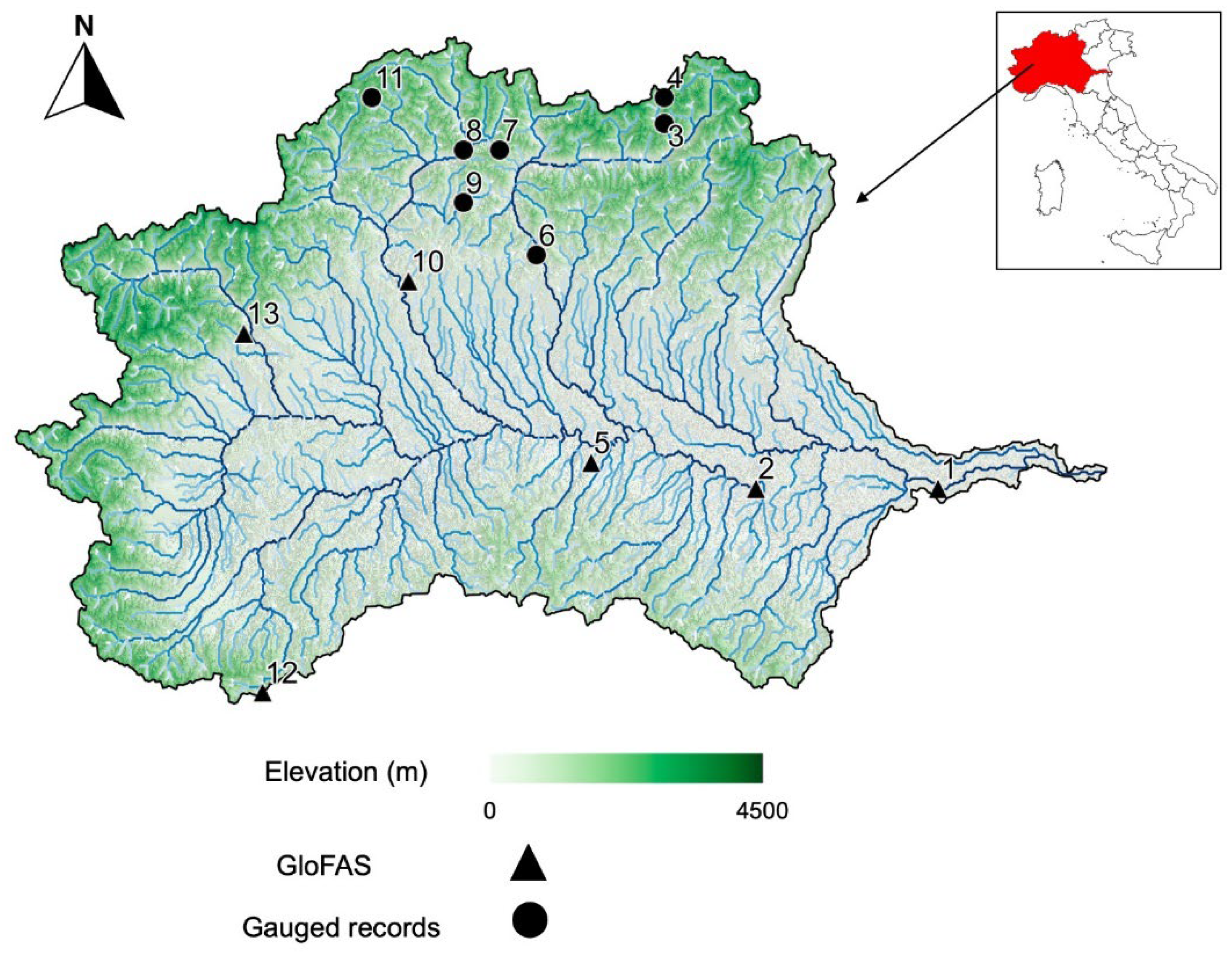
The Po River Basin (PRB) (Figure 1), located in northern Italy between the Alpine and Apennine mountain chains, is the largest watershed in Italy, covering ~74,700 km² (~71,000 km² in Italy and ~3000 km² in Switzerland and France). The mean annual temperature varies between 5 and 15 degrees Celsius, being closer to 5 degrees Celsius in the Alpine region and to 10–15 degrees Celsius in the Apennine region [1]. The mean annual precipitation is about 1200 mm, and the annual average discharge (during the period from 1923 to 2006) was 1500 m³/s, with a maximum recorded peak flow of 10,300 m³/s at Pontelagoscuro (close to the city of Ferrara) in 1951. The hydrological system of the PRB [2] is highly complex and includes a variety hydroclimatic regimes: (1) the Alpine reaches, which are snow-dominated and fed by snow and glacial melt, presenting a typical seasonal peak flow between spring and early summer; (2) the Apennine rivers, which are dominated by rainfall, showing a minimum seasonal flow during the summer; and (3) the deltaic system of the Po River [3], which is one of the most important in the Mediterranean Sea, covers an area of ~700 km², and is part of the UNESCO Man and Biosphere (MAB) Program. The interactions of this variety of hydroclimatic regimes together with the groundwater flow determine the annual regime of the Po River, which results in two hydrometric low-level periods (winter and summer) and two periods of flooding (late fall and spring).

The Po River basin is one of the most intensively populated, cultivated and highly developed areas of Europe. It hosts a total population of ~20 million people (the demographic density is ~225 inhabitants per km²), and 35% of the valued-added economic production in Italy is located within the PRB [4], including agriculture, manufacturing, and service providers. Water resource quantification and management is therefore crucial in such a watershed, given the high population density, intense agricultural land use, and hydro/thermal power plants (the majority are located in the upper PRB), where concurrent water uses have to be satisfied [4,5]. Specifically: (1) the agricultural production of the PRB represents 35% of the total national production [2] and (2) the basin contains 890 hydropower plants, which produce 46% of the total Italian hydropower production, and 400 thermal power plants, which produce 32% of the total Italian power production [2].

Given the importance of the PRB to its residents and the Italian economy, the ability to provide PRB water managers and planners information about PRB streamflow variability for increased timescales (paleo records) would be incredibly beneficial. Streamflow reconstructions using paleo proxies are limited in this region, with the most recent work [6] focusing on the Rhine River Basin (RRB) and the PRB. Obertelli (2020) [6] observed mixed results in obtaining good reconstruction skill in the RRB and poor reconstruction skill in the PRB. He attributed the poor PRB reconstruction skill to the influences of Alpine runoff [6]. Thus, the motivation of the current research was to attempt to improve reconstruction skill in the PRB by (1) using an increased search radius for the consideration of proxies to use in reconstruction models; (2) utilizing singular value decomposition (SVD) as a data reduction tool and to generate a single vector to represent PRB streamflow variability, thus developing a regional (not gauge-based) PRB streamflow reconstruction; (3) developing regional PRB streamflow reconstructions for two periods of record for the comparison and evaluation of their influence on the results; and (4) applying and evaluating a rigorous group of statistics to alleviate concerns of model multicollinearity and over-fitting.

While traditional reconstructions of streamflow rely on tree-ring proxies, [7,8] developed a novel approach at both the basin scale (i.e., Missouri River Basin, U.S.) and the continental scale (i.e., Continental U.S. or CONUS), in which tree-ring-based reconstructions of the summer Palmer Drought Severity Index (PDSI) were used as reconstruction proxies. The PDSI data were obtained from the Living Blended Drought Atlas (LBDA) [9], an updated version of the North American Drought Atlas [10], and the LBDA has a spatial resolution of 0.5 degrees by 0.5 degrees across the CONUS. In [7], the authors selected a search radius of 450 km from the streamflow gauge of interest and considered all LBDA PDSI cells within this radius when developing reconstruction models. In Europe, the Old World Drought Atlas (OWDA) provides annual June–July–August (JJA) self-calibrating Palmer Drought Severity Index (scPDSI) values for 5414 grid points across Europe from 0 to 2012 AD [11]. Similar to [6], the current research utilized the OWDA scPDSI as reconstruction proxies. While [6] limited the consideration of OWDA scPDSI cells to (only) those within the PRB watershed, the current research considered OWDA scPDSI cells within a 450 km search radius of the centroid of the PRB, per [7].

Perhaps the biggest challenge [7] identified when utilizing the LBDA as a reconstruction proxy was the high spatial correlation of the LBDA grid cells, which could lead to multicollinearity challenges in reconstruction model development. Various statistical techniques exist to determine the relationship between two spatial-temporal fields, including regularized canonical correlation analysis (rCCA), as selected by [7], and principal component analysis (PCA), as selected by [6], which are both very appropriate. Singular value decomposition (SVD) has the advantage of being able to evaluate the cross-covariance matrix of two spatial-temporal fields to identify similarities between them, while PCA evaluates only one spatial-temporal field. In [12], the authors concluded that singular value decomposition (SVD) was simple to use and preferable for general use, while [13] found that SVD was a powerful technique that isolates the most important modes of variability, and multiple studies have applied SVD in the field of hydrology [14]. SVD accomplishes two roles in that it serves as a data reduction tool for identifying significant spatial cells (i.e., independent variables—scPDSI) for use in the regression-based reconstruction models and generates a single time-series vector that represents the variability of streamflow for the multiple gauges identified in the PRB (i.e., the dependent variable). Ho et al. (2016) [7] noted that, “A single reconstruction model would be advantageous in its ability to consider all streamflow stations at once rather than fitting 55 individual models.” Thus, the novel use of SVD addresses a desire of [7] to generate a regional reconstruction instead of individual gauge reconstructions. The SVD-generated single time-series vector, which represents regional (multigauge) PRB streamflow variability, was utilized as the dependent variable in the regression-based reconstruction model, while the scPDSI cells identified by SVD served as the independent variables. The regional reconstruction complements [6], who developed PRB reconstructions at Global Flood Awareness System (GloFAS) points within the PRB for the 1979 to 2012 period. For the current research, two periods were selected for reconstruction model development: the short period of record (SPRO), similar to [6], from 1980 to 2012 (33 years), which includes thirteen PRB streamflow gauges, and the long period of record (LPRO) from 1967 to 2012 (46 years), which includes six PRB streamflow gauges. A rigorous set of statistics evaluated the developed regression models to alleviate concerns of over-fitting and multicollinearity, per [7].

2. Materials and Methods

Streamflow data consisting of the average annual flowrate (m³/s) were identified for thirteen gauges within the PRB (Figure 1 and

Table 1. Streamflow gauge information (gauge #, river, station name, country, latitude (^o), longitude (^o), area (square kilometers), elevation (meters), GloFAS data supplemented, PRBQ SPOR R², and PRBQ LPOR R²).

Gauge #	River	Station	Country	Lat	Lon	Area	Elev	GloFAS	PRBQ R2 (SPOR)	PRBQ R2 (LPOR)
1	Po, Fiume	Pontelagoscuro	IT	44.9	11.6	70,091	8	X	82%
2	Po, Fiume	Boretto	IT	44.9	10.6	55,183	20	X	88%
3	Poschiavino	Le Prese	CH	46.3	10.1	169	1015		54%	66%
4	Poschiavino	La Roesa	CH	46.4	10.1	14	1908		56%
5	Po, Fiume	Piacenza	IT	45.0	9.7	42,030	42	X	82%
6	Adda, Fiume	Lake Como Outlet	IT	45.8	9.4	4508	197		84%	94%
7	Riale Di Roggiasca	Roveredo	CH	46.2	9.2	8	1030		74%	81%
8	Ticino, Fiume	Bellinzona	CH	46.2	9.0	1515	270		83%	91%
9	Cassarate	Pregassona	CH	46.0	9.0	74	341		65%	75%
10	Ticino, Fiume	Miorina	IT	45.7	8.7	6655	190	X	81%
11	Riale Di Calneggia	Cavergno	CH	46.4	8.5	24	940		64%	81%
12	Tanaro, Fiume	Ponte Di Nava	FR	44.1	7.9	148	803	X	58%
13	Dora Baltea, Fiume	Tavagnasco	IT	45.5	7.8	3313	263	X	48%

). For measured data, we used the Global Run-off Data Center (GRDC) (http://www.bafg.de/GRDC/, accessed on 1 June 2022) discharge dataset. For each of the gauged stations, we also extracted modeled continuous streamflow data (1980 to 2012) from the Global Flood Awareness System (GloFAS) [15] (https://cds.climate.copernicus.eu/cdsapp#!/dataset/cems-glofas-historical?tab=overview, accessed on 1 June 2022). Seven of the thirteen gauges provided complete data for the period of record of 1980 to 2012. Data for six of the thirteen gauges were supplemented with GloFAS data if, for the overlapping period of the gauge and GloFAS annual streamflow, the Nash–Sutcliffe Efficiency (NSE) statistic exceeded 0.50 and the percentage bias (PBIAS) was between ±15 and ±25 [16]. Table 1 identifies the gauges with complete records and gauges with supplemented GloFAS data. The streamflow data consisted of both impaired and unimpaired gauges to increase the spatial coverage within the PRB. The use of this streamflow data was justified based on intercorrelations between the thirteen gauges for the 1980 to 2012 period of record (33 years or short period of record—SPOR), exceeding 99% significance for 72 of 78 combinations, with the six outliers achieving significance levels ranging from 93% to 98%. A subset of six PRB gauges were identified with a period of record of 1967 to 2012 (46 years or long period of record—LPOR) (Figure 1 and Table 1).

The Old World Drought Atlas (OWDA) provides annual June–July–August (JJA) self-calibrating Palmer Drought Severity Index (scPDSI) values for 5414 grid points across Europe from 0 to 2012 AD [11]. Similar to [7], the current research utilized the OWDA scPDSI as a proxy for PRB streamflow reconstructions and included 195 scPDSI cells within a 450 km search radius of the centroid of the PRB.

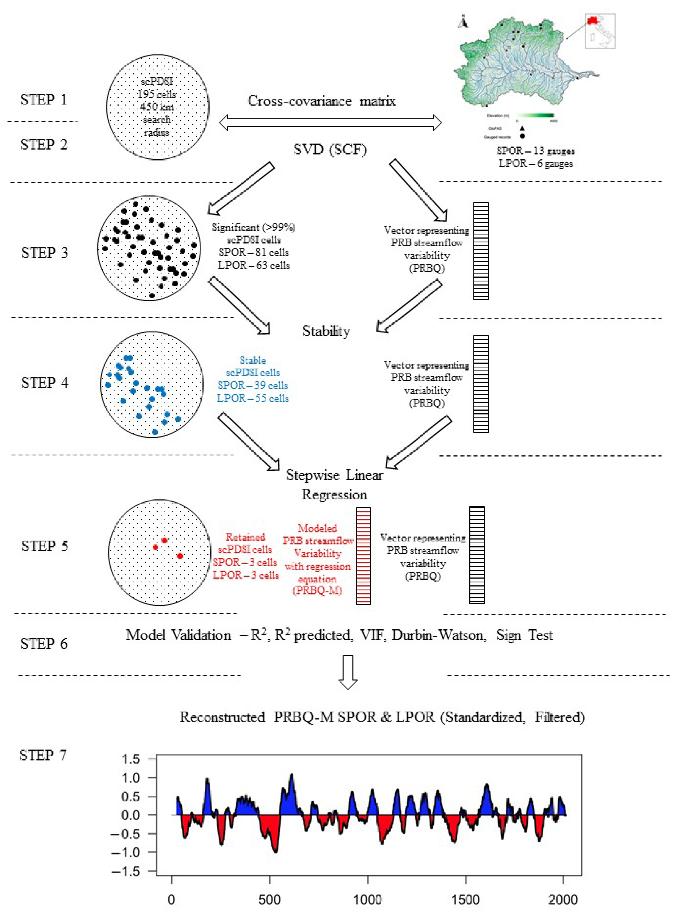
SVD is a multivariate technique for identifying relationships between two spatial-temporal fields [12]. In the field of hydrology, early applications of SVD included the evaluation of sea surface temperatures (SSTs) and precipitation [17], and SSTs and drought [18]. Two matrices (a matrix of standardized scPDSI anomalies and a matrix of standardized annual streamflow anomalies) were developed, in which the time dimension of each matrix (i.e., 33 years for the SPOR or 46 years for the LPOR) must be equal. The cross-covariance matrix was then computed (Figure 2—STEP 1), and SVD was applied (Figure 2—STEP 2), which resulted in two matrices of singular vectors and one matrix of singular values (1st mode, 2nd mode, etc.). The squared covariance fraction (SCF) is a useful measurement of the importance of modes [12]. Each singular value was squared and divided by the sum of all squared singular values to produce a fraction (or percentage) of squared covariance for each mode. If the leading three (e.g., 1st, 2nd, and 3rd) modes explain a significant amount (i.e., >80%) of the variance in the two fields, then SVD can be utilized [19] (Figure 2—STEP 2). The two matrices of singular vectors were examined, generally referred to as the left (i.e., scPDSI) matrix and the right (i.e., streamflow) matrix. The first column of the left matrix (1st mode) was projected onto the standardized scPDSI anomalies matrix, and the first column of the right matrix (1st mode) was projected onto the standardized streamflow anomalies matrix. This resulted in the 1st temporal expansion series (TES) of the left and right fields, respectively, and they are referred to as the left 1st TES and the right 1st TES (hereafter referred to as PRBQ). Each TES vector has dimensions of one by the number of years (i.e., either 33 years or 46 years). The left heterogeneous correlation values (for the 1st mode) were determined by correlating the scPDSI values of the left matrix with PRBQ, and utilizing the approaches of [17,18], heterogeneous correlation figures displaying significant correlation values for scPDSI were developed (Figure 2—STEP 3). While SVD is an incredibly effective statistical tool for data reduction and identifying significant scPDSI grid points, the PRBQ represents a single vector of annual streamflow variability, accounting for all gauges (either thirteen or six) in the PRB.

SVD identified significant scPDSI cells for both SPOR and LPOR, and cells of 99% significance or greater were considered for use in the reconstruction model. Prior to input into the reconstruction model, a final prescreening method was applied to investigate temporal stability, per [20], which consisted of performing correlations over moving windows between the PRBQ and the retained scPDSI cells for both the SPOR and LPOR (Figure 2—STEP 4). A thirty-year moving correlation window was selected by [21,22]. However, in [22] the average streamflow record was ~77 years in length. Thus, the thirty-year moving correlation window was ~40% of the total period of record. The authors selected a conservative and more rigorous moving correlation window of approximately one third (~33%) for the SPOR (an 11-year moving correlation window) and the LPOR (a 15-year moving correlation window). A stability analysis ensured that reliable and practical streamflow reconstructions were generated.

A forward and backward stepwise linear regression (SLR), per [21,22,23] (Figure 2—STEP 5), was used to develop models for the reconstructions, and various statistics were used to test model skill (Figure 2—STEP 6). R² (model variance), R² predicted (drop-one cross-validation) [24], the variation inflation factor or VIF (1 to 10 reveals a low correlation between predictors and predictand) [25], the Durbin–Watson (D–W) statistic, which tests for autocorrelation [26], and the sign test, which counts the number of agreements and disagreements between observed and reconstructed (modeled) flow, were used for model validation. The modeled flow was standardized, and a 30-year end-year filter was applied (Figure 2—STEP 7).

3. Results

SVD Model: The cumulative SCF for the first three modes was 98% for the SPOR and 99% for the LPOR, and generally, if the first three modes explain a significant (greater than 80%) amount of the variance between the two fields, then SVD can be applied to determine the strength of the coupled variability present [19]. The 1st mode of SCF was 90% for the SPOR and 94% for the LPOR. Thus, only results for the first mode were provided.

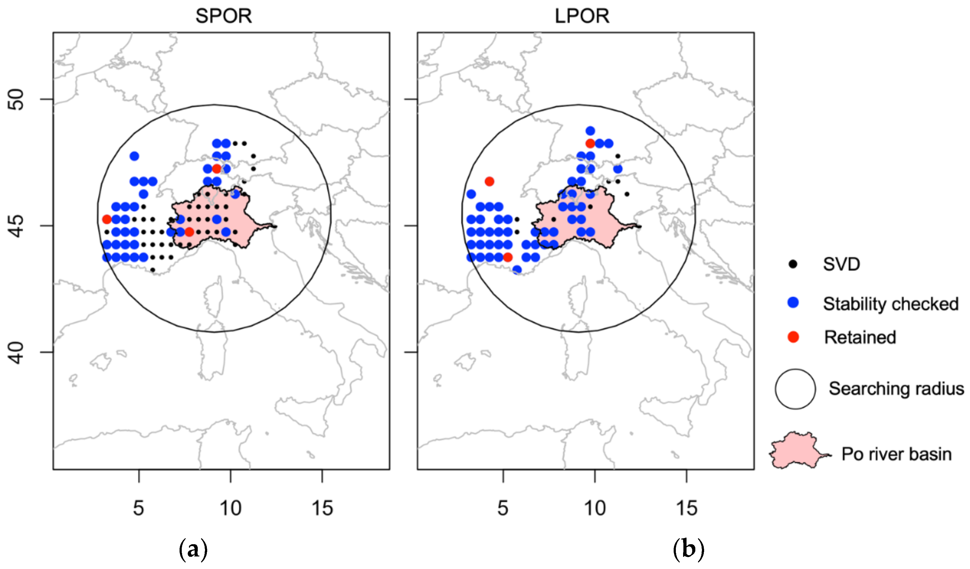
scPDSI—For the 1st mode, scPDSI correlation maps for both the SPOR and LPOR were developed, and cells exceeding 99% significance (SPOR—81 cells and LPOR—63 cells) were identified (Figure 3a,b).

Streamflow—For both the SPOR (thirteen gauges) and LPOR (six gauges), all gauges exceeded 99% significance. The PRBQ vectors, generated via SVD for use as regional reconstructions, were developed for both the SPOR and LPOR. For the SPOR, the PRBQ vector was correlated with each of the thirteen gauges, and the R² values are provided in Table 1. This was repeated for the LPOR such that the PRBQ vector was correlated with each of the six gauges, and the R² values are provided in Table 1. As displayed in Table 1, the SVD-generated PRBQ vector, for both the SPOR (average R² = 71%) and the LPOR (average R² = 81%), captures a high degree of the variability of the individual streamflow gauges. Thus, the use of the PRBQ vector was appropriate as a regional representation of PRB streamflow variability for both the SPOR and LPOR.

Predictor Prescreening: For the SPOR, the 11-year moving-window correlation analysis of the 81 scPDSI cells and the PRBQ vector identified by SVD, 39 scPDSI cells were deemed stable and were considered for the SLR model (Figure 3a). For the LPOR, the 15-year moving-window correlation analysis of the 63 scPDSI cells and the PRBQ vector identified by SVD, 55 scPDSI cells were deemed stable and were considered for the SLR model (Figure 3b). It was notable that the majority of the stable cells were spatially located west and within the PRB, verifying the general climate (moisture) signal of a west-to-east movement.

Reconstruction Models: The reconstruction of the SPOR regional PRBQ annual streamflow vector resulted in exceptional statistical skill. The SLR model retained three scPDSI cells (#44, #111, and #140) (Figure 3a). Model results of R² = 0.77; R² predicted = 0.69; VIF = 1.0; D-W = 1.71 (Pass); Sign Test 15+/18- (Pass) and a model equation of PRBQ − Modeled (SPOR) = 0.301 + 0.783 * scPDSI (44) + 0.477 * scPDSI (111) + 1.100 * scPDSI (140) were obtained. The reconstruction of the LPOR regional PRBQ annual streamflow vector again resulted in strong statistical skill. The SLR model retained three scPDSI cells (#14, #54, and #167) (Figure 3b). Model results of R² = 0.65; R² predicted = 0.56; VIF = 1.0; D–W = 1.69 (Pass); Sign Test 22+/24- (Pass) and a model equation of PRBQ − Modeled (LPOR) = −0.020 + 0.355 * scPDSI (14) + 0.454 * scPDSI (54) + 0.795 * scPDSI (167) were obtained.

The SPOR and LROR models were standardized, and a 30-year end-year filter (moving average) was applied (Figure 4). Referring to Figure 4, each reconstruction generally captured similar drought and pluvial periods. The end of the 5th century to the beginning of the 6th century reveals a megadrought period peaking around ~530 AD, with the SPOR model showing a greater decline when compared to the LPOR model. Interestingly, the most robust pluvial period immediately followed this megadrought and peaked around ~610 AD.

The relative agreement (visual assessment of Figure 4) between the two models (SPOR and LPOR) was encouraging, given (1) two different periods of record were evaluated and independent regression models were generated for each; (2) the gauges used for the SPOR reconstruction were spatially distributed across the entire PRB, while the gauges used for the LPOR reconstruction were generally more associated with Alpine streamflow; (3) each model (SPOR and LPOR) retained three scPDSI proxies, and for each model the retained scPDSI proxies (cells) differed; and (4) the reconstruction skills for both models were strong, and each model passed a rigorous assessment of multicollinearity and over-fitting.

4. Discussion

In a recent paleo study in which streamflow was reconstructed for multiple watersheds across Europe [27], drought years were consistently identified in 1540, 1669, and 1921. We compared the results from the PRB to [27] and, per

Table 2. Drought periods (1-year, 5-year, 10-year, 20-year, and 30-year) for the PRB regional reconstruction from 0 to 2012 AD. The number in the parenthesis represents the drought period ranking.

Time Period (AD)	1-Year	5-Year	10-Year	20-Year	30-Year
0 to 100
100 to 101
201 to 300	242 (4)	249–245 (2)		254–235 (4)	254–225 (2)
301 to 400
401 to 500
501 to 600		527–523 (5)	512–503 (4)	511–492 (2)	532–503 (1)
601 to 700
701 to 800
801 to 900			848–839 (5)
901 to 1000
1001 to 1100				1067–1048 (3)	1073–1044 (3)
1101 to 1200
1201 to 1300
1301 to 1400	1385 (1)
1401 to 1500				1426–1406 (5)	1444–1415 (4)
1501 to 1600	1503 (2) 1540 (11)
1601 to 1700	1669 (130)	1687–1683 (1)	1687–1678 (2)
1701 to 1800	1784 (5)
1801 to 1900		1865–1861 (3)	1865–1856 (1)	1875–1856 (1)	1876–1847 (5)
1901 to 2012	1921 (3)	1950–1946 (4)	1952–1943 (3)

, the 1921 drought ranked #3, the 1540 drought ranked #11, and the 1669 drought ranked #130. Thus, the current research identified similar drought years to [27]. The 6th century appears to be the driest period in the ~2000 year reconstruction, as multiple drought events for various filters are displayed in Table 2, with the most extreme megadrought being from 503 to 532 (30-year period). Future research will investigate the current (2022) drought and, in particular, the development of the regional reconstructions of the PRB per the current research, coupled with detailed climatological and hydrological studies, will allow for the quantification of this drought and the comparison of 2022 to both observed and paleo-derived streamflow records.

5. Conclusions

A skillful reconstruction of the PRB annual regional streamflow was developed. Obertelli (2020) [6] developed annual streamflow reconstructions for GloFAS sites (27 grid points) with an average R² of 0.36. The current research developed two reconstructions of PRB annual regional streamflow that achieved R² values of 0.77 and 0.65. The improvement in skill was likely attributed to including scPDSI cells within a 450 km search radius, per [7], whereas [6] limited the inclusion of scPDSI cells to those within the watershed. Five of the six scPDSI cells retained in the SLR models were spatially located outside the PRB watershed, thus limiting the search to (only) scPDSI cells within the PRB watershed, per [6], likely limited the reconstruction skill. The novel use of SVD allowed for the development of regional PRB annual streamflow vectors for both the SPOR and LPOR, which were highly correlated with the individual PRB gauges. We suspect that a regional representation of PRB streamflow improved statistical skill when compared to individual gauges or GloFAS grid points. The two reconstructions of annual PRB regional streamflow were developed independently, yet displayed similar temporal variability, which was encouraging.