1. Introduction
Community science research relies on data collected and submitted by community volunteers and is an increasingly popular tool to collect scientific data, involve the community in scientific research, and provide information and education about a prominent issue [
1,
2]. The process was arguably first employed to engage the public and extend the reach of science at the turn of the 20th century with the Cooperative Weather Service (since 1890) and the National Audubon Society Christmas Bird Count (since 1900) [
2]. Since then, community scientists have been active in long-term ecologic population counts, phenologic studies to assess impacts of climate change, and inventories of invasive and rare plants [
3]. In the US, community scientists have focused more on monitoring environmental quality over single species monitoring [
4]. More recently, one-time events and collective problem-solving activities have become popular, including data blitzes that generate substantial data over a short time period and online participatory events that engage the larger global community, including those with mobility constraints [
5].
In hydrology, recent community science projects include collection of stage data [
6,
7,
8,
9], flood risk analysis [
10], and capture of community perspectives of watershed issues [
11], among others. In one study, youth were tasked with documenting local watershed issues of perceived importance using Photovoice, and photos were later data-mined to distill the youth perspective [
11]. Such community science research shares a common purpose: community members collaborate in scientific research to meet real-world goals that support conservation, raise environmental awareness, or inform policy decisions [
5]. A thorough review of community science applications to hydrology, including opportunities for water quality monitoring, discharge monitoring, mapping, and conflict resolution, is available in [
1]. A more recent review examines benefits and obstacles in community science, classifying projects as related to geohazards, observation/classification, education/outreach, and other foci [
12].
Benefits of community science activities include increasing the reach of scientific monitoring and supporting science outreach and education while producing reliable research data. One concern with use of contributed data is data quality [
13] and assessing uncertainty in data [
12]. Using data from the CrowdHydrology network [
6], a decision tree approach was applied to evaluate and clean submitted data, yielding estimates of data uncertainty [
14]. In a separate study, data quality in community science were examined and it was concluded that datasets produced by volunteers can be of comparable quality to those produced by professionals, provided methods to boost accuracy and account for bias are in place [
2]. They suggest employing iterative design, using simple and systematic tasks, recording of metadata, accounting for collection effort variability, and comparing with data collected by professionals as appropriate methods to ensure data quality. Therefore, dual goals of education/outreach and scientific research are achievable in collaborative community science projects.
One difficulty in processing volunteered geographic information is in adding reported data to a database. This may be resolved through use of freely available data collection apps developed for a specific purpose, e.g., iNaturalist and eBird for biodiversity data [
15,
16]. It may also be resolved through use of web-based mapping utilities [
17] such as ArcGIS products used to map visual pollution in urban settings [
18] or contribute data to a global Landslide inventory [
19]. The necessity of smartphone use may, however, be a barrier to participation for some aspiring community scientists. One solution is to accept data submitted via text message, as with CrowdHydrology [
6], following with an automated process to parse the data and enter them into the project database. This is the approach used in the present study.
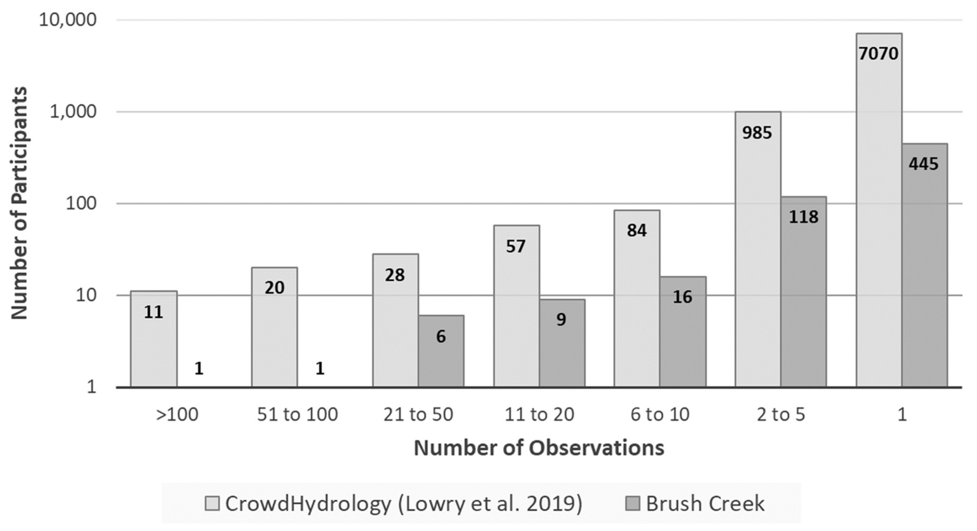
In this study we describe a free automated system to collect stream stage data contributed by community scientists and match it with weather data to build a database of rainfall and stream stage. These data may then be used to assess both the stream’s hydrologic response to rainfall and patterns in community science data contribution. In particular, the question of who contributes data is of interest. Lowry et al. (2019), reporting on data submission patterns in the CrowdHydrology project [
20], found 86% of participants contributed data only once, with 0.1% of participants classed as “champions” who contributed over 100 observations each, and accounting for 19% of contributed data. We seek to assess whether participation in this project breaks down in an equivalent manner.
The aims of the study are, therefore, to (1) identify temporal and individual patterns of community science observations and (2) develop a statistical model of stream stage using antecedent rainfall data and stage observations from community scientists.
2. Materials and Methods
2.1. Study Area and Flood History
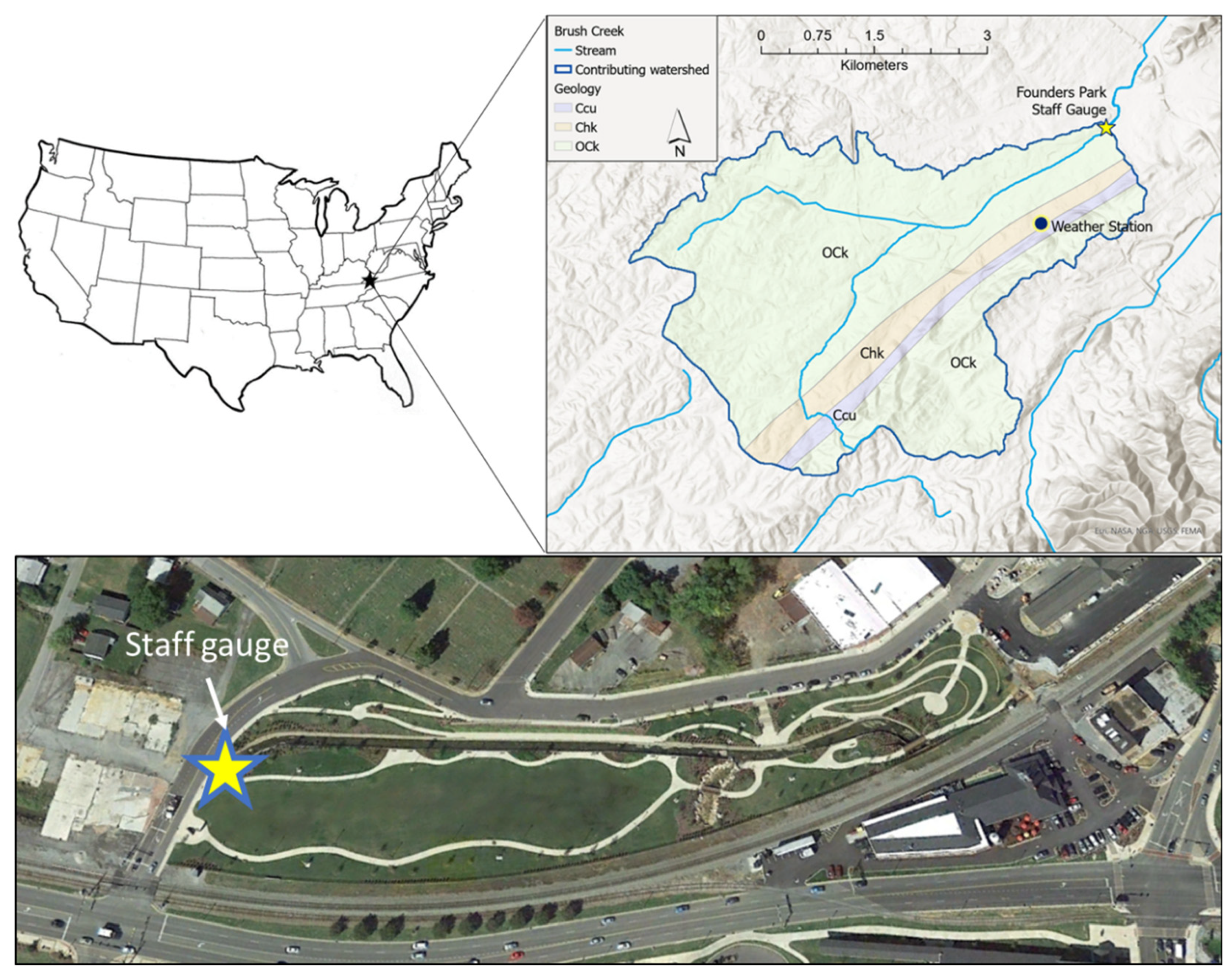
The research was conducted on Brush Creek in Johnson City, Tennessee, USA (HUC 060101030505). The stream’s 42 km2 watershed (with a contributing area of 19.2 km2 upstream of the staff gauge used in this study) has an average gradient of 11.4 m/km and flows through the historic downtown. The Time of Concentration to the measurement point at the staff gauge is 84 h.
The watershed is in the Valley and Ridge physiographic province, consisting of a series of northeast-southwest trending shale and sandstone ridges and carbonate valleys. Bedrock in the Brush Creek watershed consists of carbonates of the Knox and Honaker dolomites (OCk and Chk, respectively) with a small ridge of the shale and dolomite Conasauga formation (Ccu) running parallel to the strike (
Figure 1). Elevation ranges from 617 m in the southern ridges to 494 m at the staff gauge and the longest flow path is 9 km. The region experiences a humid continental (Köppen Cfa) climate with year-round precipitation and hot summers. Average annual precipitation is 1070 mm and annual average temperature ranges from 1.1 °C in January to 23.3 °C in July.
Brush Creek has an extended history of flooding dating back over one hundred years [
21]. From 1901 through 1956, sixteen flooding events were recorded, with the largest events in 1908 (56.1 m
3/s) and 1938 (62.3 m
3/s) [
21]. These largest recorded events were several orders of magnitude greater than the typical discharge of 0.33 m
3/s (per a US Geological Survey stream gage 3486500 operational from 1932–1934). There are currently no gauging sites on Brush Creek.
To address continued flooding following the 1959 report, in 2001 Johnson City set out to study the causes and solutions to flooding along Brush Creek in downtown Johnson City [
22]. Water surface elevations resulting from the 10-year (0.1 annual probability) and 100-year (0.01 annual probability) 24-h storm events were modeled using the EPA Stormwater Management Model (SWMM) Version 4.4, from rainfall intensity, soils, and land use data. Hydrographs for the design storms were generated from model output, and the model was calibrated and validated using data from local rainfall events, including a 2003 flood during which a total of 119 mm of rain was measured at East Tennessee State University (ETSU), 1.9 km upstream. Various mitigation measures to address flooding were presented to the city and to residents during public meetings, and the recommended option was to develop a downtown Greenway to spur economic development and to address flooding.
In 2008, AMEC Earth & Environmental, Inc. was contracted by the City of Johnson City to complete a second downtown drainage study to assess whether a “relatively minor capital improvement project” could help to alleviate some of the flooding problems that have plagued the downtown area since the late 1800s [
23]. The 2008 study confirmed the findings of the 2005 CDM study [
22], concluding that a major capital outlay would be needed to provide flood relief for the downtown area. AMEC used the SWMM model developed in the 2005 CDM study to perform hydraulic simulations of water levels using 24-h rainfall totals with the goal of assessing the efficacy of various flood mitigation concept scenario in controlling flooding in the downtown corridor. The report recommended a phased approach that combined (1) storage ponds and bypass culverts for a tributary stream, King Creek (5-year flood protection), (2) a new open channel to replace the old Brush Creek culvert (25-year flood protection), and (3) construction of three regional detention ponds upstream of the downtown area to provide protection from the 0.02 to 0.01 probability flooding event (50- to 100-year flood). The estimated cost for all phases totaled US
$25.7 million [
23].
The city recently implemented phases 1 and 2 by restoring an old warehouse property. First a culvert was removed and Brush Creek, which originally flowed under the warehouse, was daylighted. The property was developed into a community space known as Founders Park. The space plays an important flood mitigation role through increased channel capacity, a large lawn for infiltration, and an amphitheater that doubles as flood storage (
Figure 1). Community buy-in for efforts to control flooding is important, and a community science project was developed in collaboration with ETSU, the City of Johnson City, and a local watershed group, Boone Watershed Partnership, to increase public awareness and collect stream stage data along Brush Creek. One important component of the data collection was to make the data available in real time to avoid delays associated with physical data retrieval from a logger or autographic stage recorder. Ultimately, access to real-time stage data can provide necessary foundation data for implementation of a flood warning system.
2.2. Field Data Collection
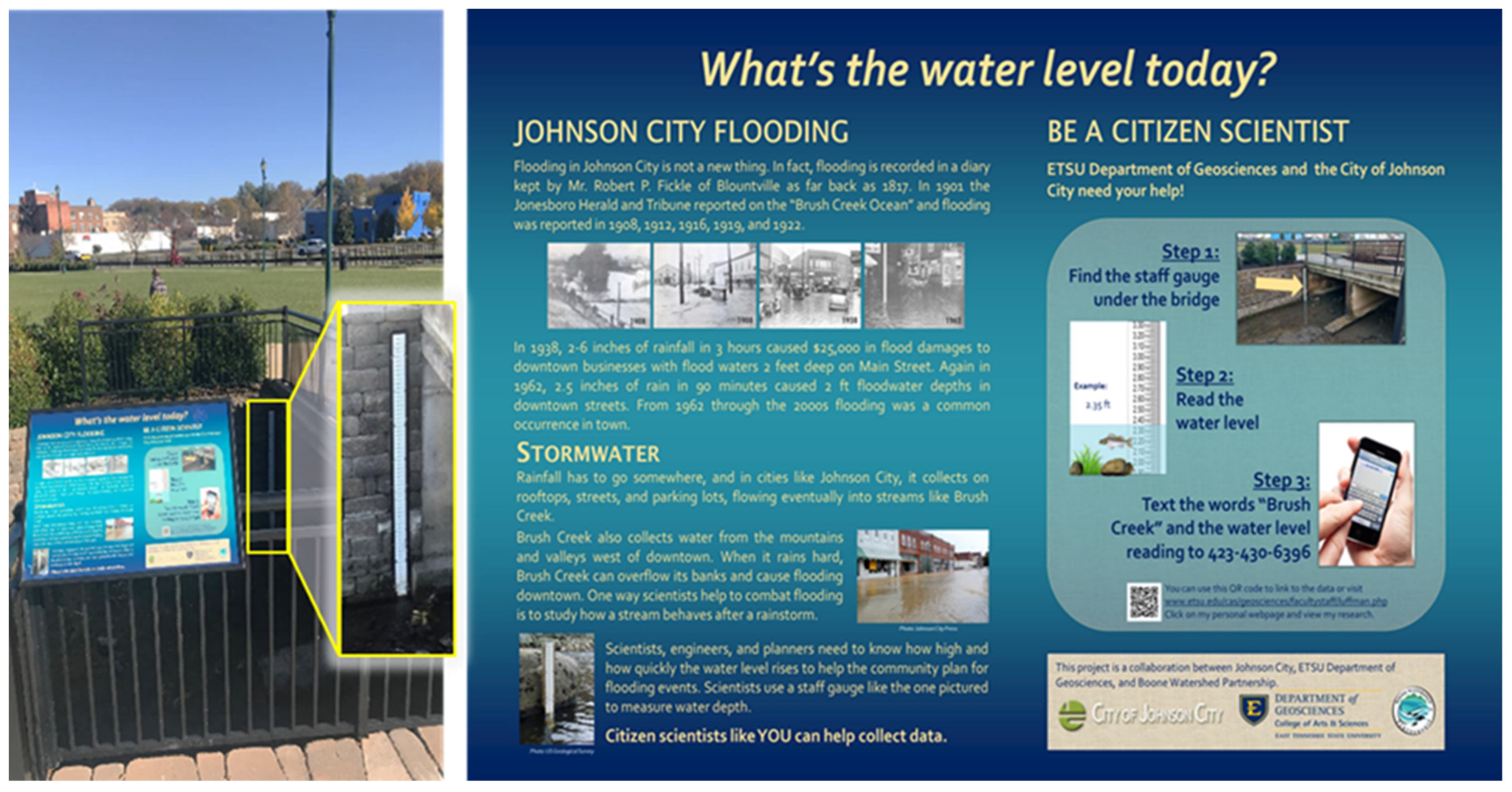
In May 2017, a staff gauge was installed on a bridge abutment at the upstream entrance to Founders Park, and a nearby sign provides details of Brush Creek’s flooding history. Instructions describe how to read the staff gauge and submit the water level reading via text message (
Figure 2). Concurrently, a Davis Vantage Pro weather station was installed on the ETSU campus within the Brush Creek watershed, 1.9 km upstream from the staff gauge. This weather station records precipitation, temperature, pressure, and wind data at 5-min intervals.
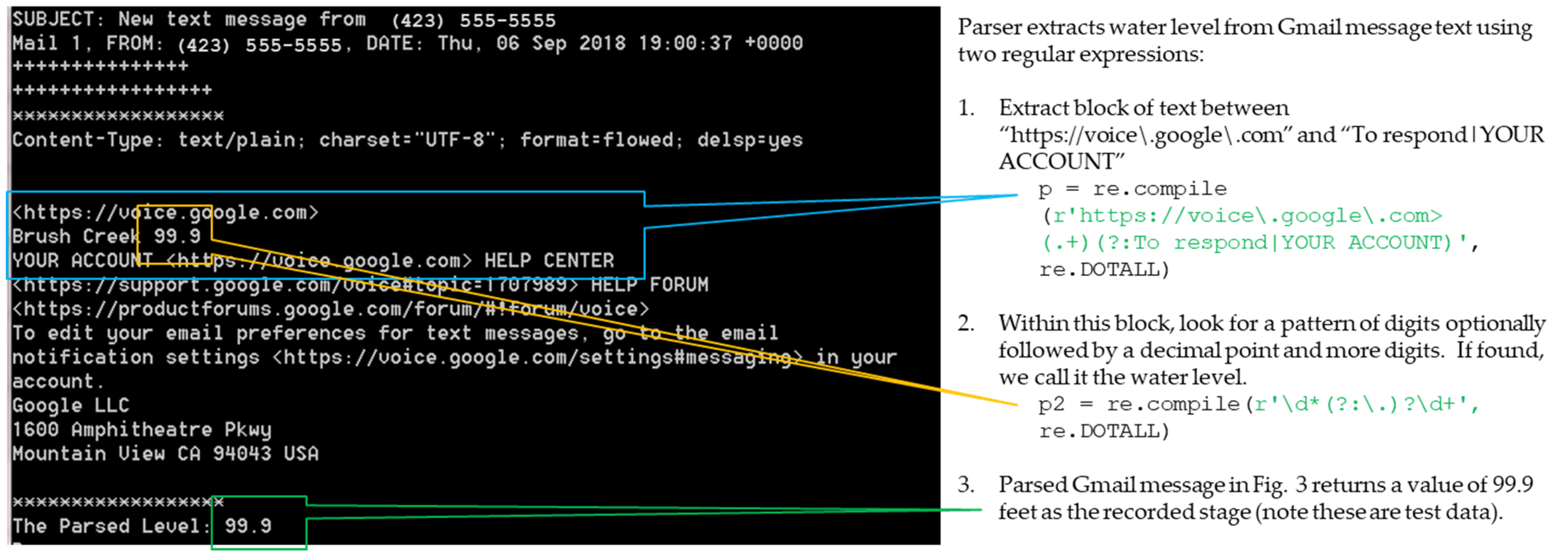
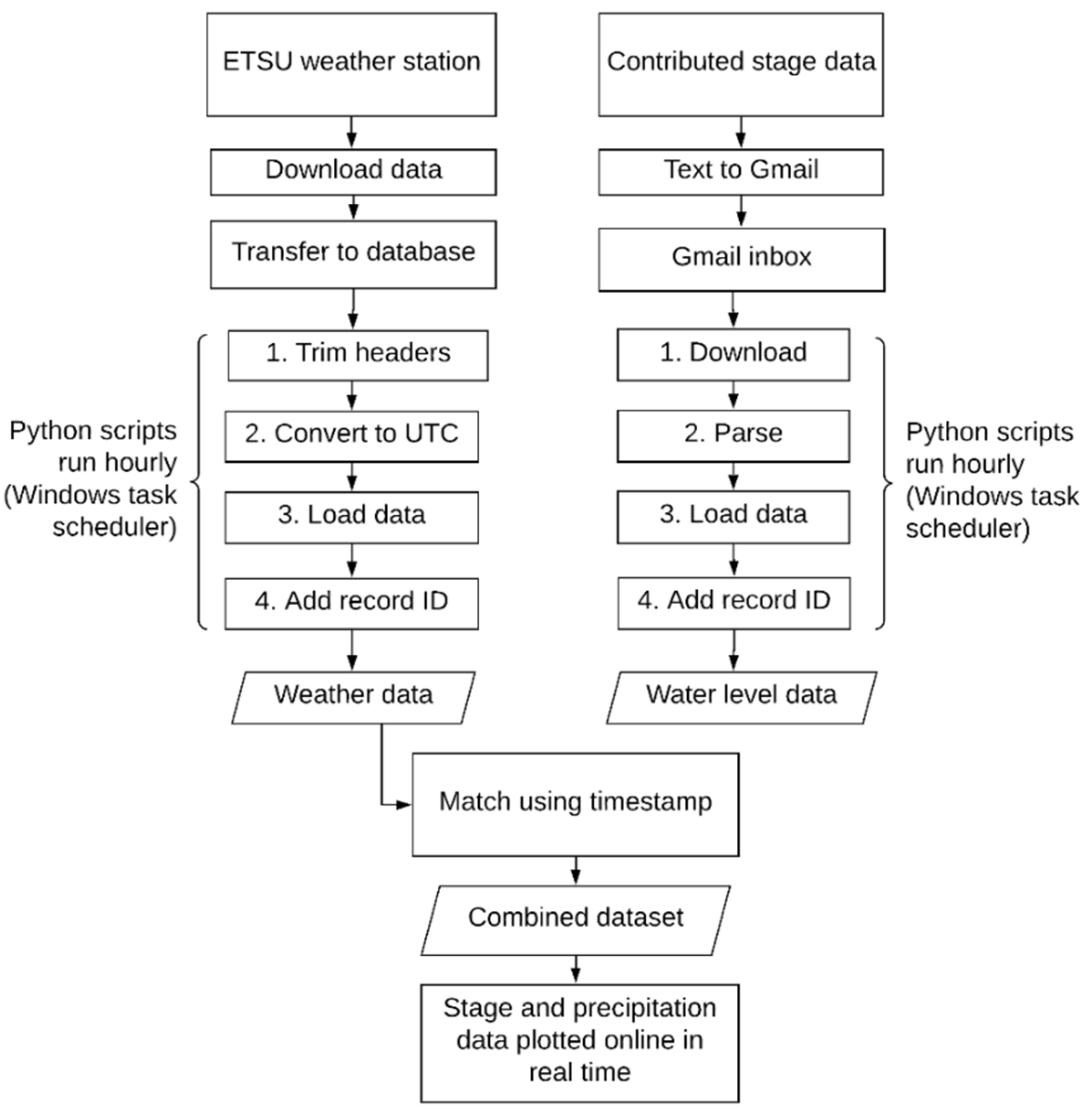
Contributed stage data observed at the staff gauge by participating community scientists are sent via text message to a Google Voice phone number set to forward to a Gmail account. Python scripts on a computer on the ETSU campus run on an automated schedule using Windows Task Manager to download the email messages. The parser uses regular expressions to extract the reported stage level from the body of the email message, and the stage, timestamp, and source phone number are written into a PostgreSQL database, populating a table of stage data.
Figure 3 shows how a representative text message appears as an email when going through the Google Voice/Gmail process. The sender’s phone number and the timestamp are easy to extract from this email. The reported stage level is extracted using two regular expressions. The first regular expression shown in Step 1 in
Figure 3 extracts the body of the actual text message along with some additional header/trailer text added by the Google Voice/Gmail process. The second regular expression shown in Step 2 in
Figure 3 is then applied to the text extracted from the first step to find the submitted stage level. Each stage data record is assigned a unique ID.
Weather data are downloaded from the ETSU weather station hourly, and Python scripts running on an automated schedule add a unique ID to each weather record. Weather data are loaded into the PostgreSQL database, populating a table of weather data. Using the timestamps, the stage data and weather data are matched, and data reports of timestamped stage and weather data are written to .csv files hourly. The complete automated workflow is shown in
Figure 4.
The software tools such as Google Voice, Gmail, Python and PostgreSQL were chosen because they are readily and freely available allowing the software part of the system to be implemented at no cost, making this system cost attractive for those wishing to replicate it.
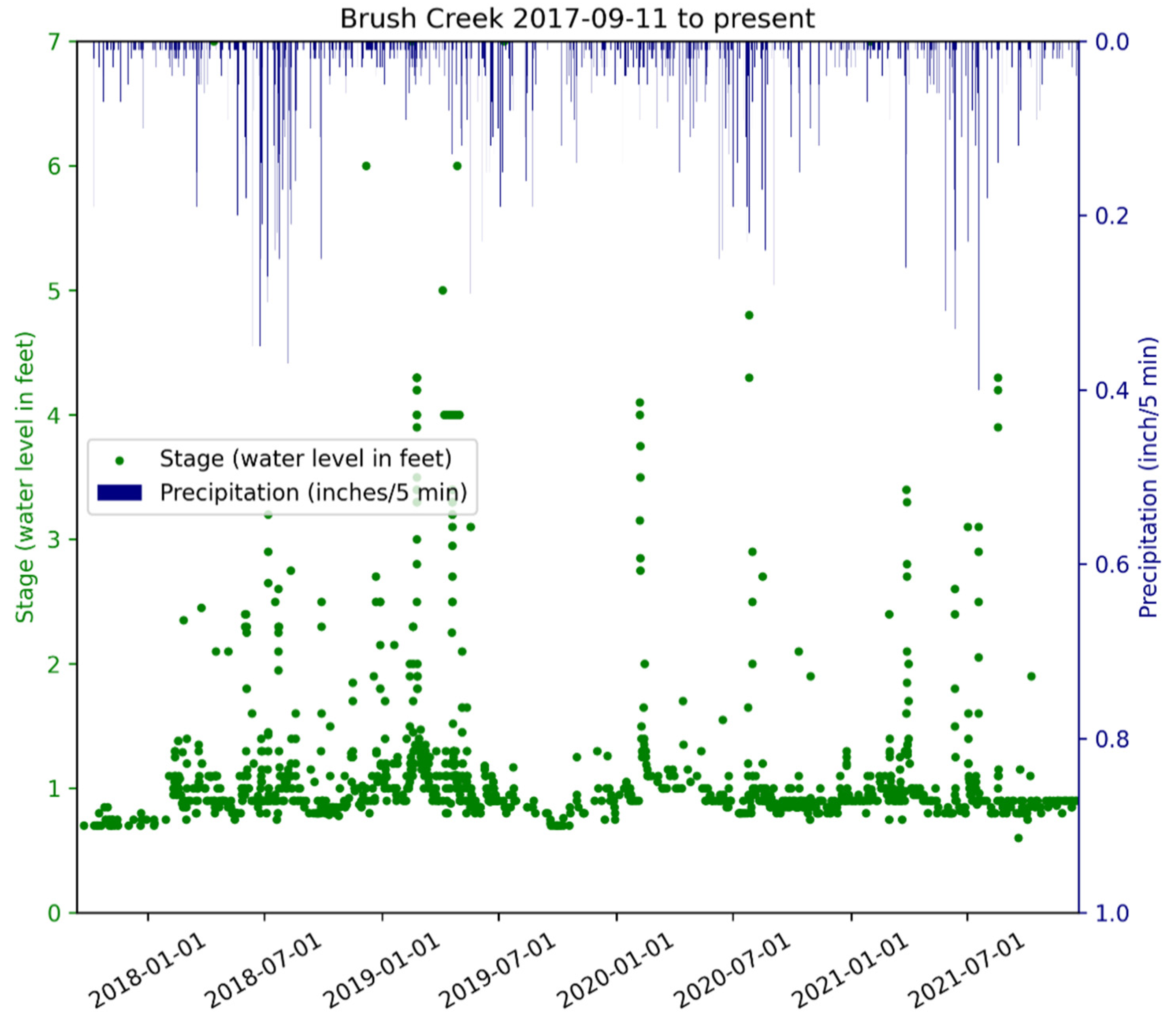
The Python plotting program Pyplot was used to plot preliminary stage and precipitation data from the hourly reports, generating five plots in real time and reflecting different time frames: all data, past year, past month, past week, and past 24 h. Prior to plotting, contributed stage data outside the range of 0.15 m to 2.1 m are excluded as these values are below baseflow and above the length of the staff gauge, respectively. Prior to formal data analyses, contributed data are reviewed and corrected. Recognizing that data accessibility is paramount to promoting and sustaining a community science project [
12], the preliminary plots are updated and uploaded hourly to the ETSU Geosciences ArcGIS server. They are available publicly online at
https://iluffman.wixsite.com/ingrid-luffman/research (accessed on 15 December 2021). A sample plot showing data from 2017-09-11 to 2021-12-15 is displayed in
Figure 5.
2.3. Assessment of Contributed Community Science Data
To assess parser performance and data quality, stage data contributed from 2017-05-17 through 2021-07-31 were compared to the parsed data and classified into three groups: (1) data were correctly parsed, (2) false positive (incorrect data extracted), and (3) false negative (parser unable to extract data even though usable data were reported) (
Figure 6). Submissions from individual participants were tallied to identify top data contributors and the frequency distribution of number of observations per participant was calculated.
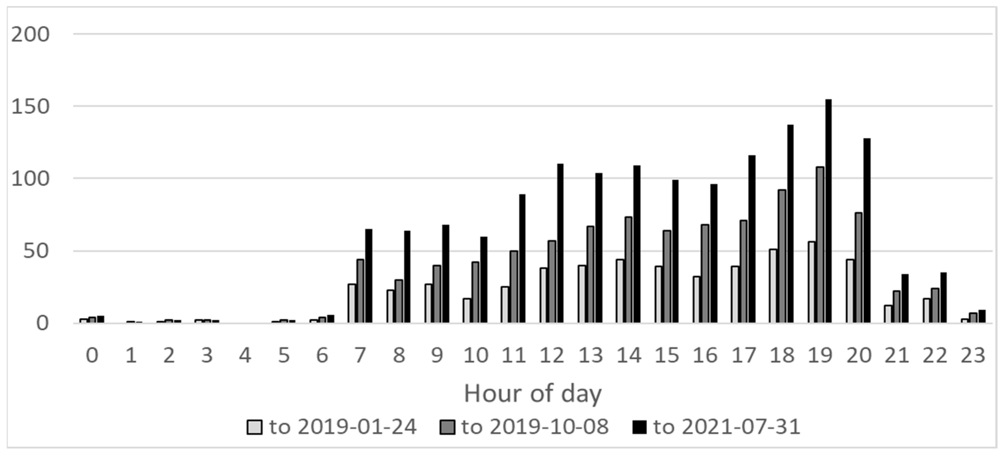
To statistically correlate precipitation accumulation to streamflow as a rainfall–runoff response, a time series dataset of both rainfall and runoff (here, using stage as a proxy) is required. The frequency of contributed stage data was assessed by cross-tabulating by day of week and time of day to identify peak days and times for community participation.
2.4. Rainfall–Runoff Response
We calculated antecedent precipitation for lags of 15 min, 30 min, 1 h, 2 h, 3 h, 6 h, 12 h, 1 day, 3 days, and 7 days prior to each stage observation. The Spearman correlation coefficient between antecedent precipitation and stage was calculated for each stage measurement. Ordinary Least Squares (OLS) regression models were developed for stage using antecedent precipitation at various lags to identify the timing of rainfall-associated runoff in Brush Creek.
4. Discussion
4.1. Assessment of Contributed Data
Successful data collection by community scientists requires context and clear unambiguous instructions. Junk data, missing data, and use of Emojis can result in false positives (wrong data extracted) and false negatives (parser unable to extract data even though usable data were reported). In this project, community scientists were encouraged to submit stream stage observations via text messaging. Simple illustrated instructions for contributing readings were provided on the educational sign (
Figure 2). When participants followed instructions for submitting stream stage data, the parser successfully parsed their texts. However, community scientists did not always follow instructions and embellished their submissions with additional text, time and date stamps, emojis and other non-Unicode symbols that can cause the regular expression-based parser to fail to properly extract the reported stream stage. Failures consisted of false positive results where the parser reported the incorrect stage and false negatives where the parser was unable to extract the stage observation from the text message. Despite the 96.7% parser success rate over the course of the project, we seek to reduce parser failures. Manual analysis of the submitted texts has identified some patterns of user submissions that lead to parser errors.
First, some community scientists entered the date or time of the observation followed by the stream stage data. The simple parser extracts the first numbers it encounters in the text message as the stream’s stage, anticipating that participants will follow the instructions provided. To address this, we recommend that the regular expression be extended to disregard numbers that look like dates or time stamps when extracting the stream stage data; numbers containing colons, dashes, slashes or a.m. or p.m. indicators could be ignored.
Second, some participants spelled out their submission, for example “one point four.” Some gave ranges, “between 1.4 and 1.5” or relative values, “a bit under 2”. Creating regular expressions to handle these latter examples is very difficult. More sophisticated natural language processing techniques would be needed to properly parse these examples.
4.2. Improving Participation
Community scientists have been encouraged to participate in this project through public outreach. With the support of Johnson City, signage was installed to publicize the project and to instruct the community on how to participate. Undergraduate students in general science education and geosciences courses at ETSU were introduced to the project and encouraged to submit data. Educational field trips have been conducted for local youth (including the Girl Scouts of America), environmentally focused organizations, and conference attendees and other academics.
Personal conversations with community members revealed that potential participants were skeptical that their stage observations were, in fact, recorded and used for research. To encourage repeat participation, in summer 2020, a “Thank you” text message was instituted. Now, within 15 min of submitting an observation, participants receive a response text thanking them for submitting data to the project. Following implementation of the “Thank you” text, participation rate doubled from 13.75 observations per month (July 2019–June 2020) to 26.88 observations per month (July 2020–June 2021).
Automated real-time plots available online and updated hourly were another effort to improve participation through engagement. Within one hour of contributing an observation, participants can view their contributed data on the data plots.
Other suggestions for improving participation focused on generating interest through rewards or badges for regular participants [
12], or by installing hands-on devices like a bicycle instrumented to serve as a generator that passersby could ride to power nearby spotlights to aid in nighttime observations, or to power internet-of-things projects.
One advantage of our methodology is the use of simple instructions (read the gauge, send a text), a widespread communication utility (text messaging), and freely available tools to handle observations (Google Voice and Gmail) and generate reports and plots (PostgreSQL and Python). This methodology is replicable in other parts of the watershed and in other communities. The sole portion of the process that uses proprietary software is our use of the ArcGIS server at ETSU to store images of the stage/precipitation plots (
Figure 4). We used this server as it was readily available, however, another server could be used.
Another advantage of our methodology is how data are transferred. The system we implemented permits the host computer to request data from Google Voice and Gmail and pull it to the host computer, process it, and push it back out to the cloud in the form of data plots. This eliminates security risks associated with pushing data from the cloud to the host computer.
4.3. Assessing Rainfall–Runoff Response
A limitation of this study is the gaps in contributed stage data that fail to capture peak flows. Nevertheless, data are sufficient to identify patterns of recession following high flows and normal base flows (
Figure 5). Occasionally, high stage values were reported by community scientists without any recorded precipitation at the ETSU rain gauge, for example, in February of 2020 (
Figure 5). This is likely the result of rainfall elsewhere in the watershed. Given the karst geology of the region, springs may also contribute water from outside the watershed, but within the springshed for Brush Creek. We recommend that data from additional rain gauges be located and included in future analyses.
Because of the sporadic timing of contributed stage data, we selected the approach of using the antecedent precipitation associated with each stage observation to evaluate the rainfall–runoff relationship. Regression models identified that precipitation in the preceding 15 min had the greatest influence on stream stage, indicating a tendency toward flashy behavior. The negative coefficient for 6-h antecedent precipitation likely reflects a quick drop in stage following peak flow associated with a rain event. Field observation of Brush Creek discharge during and immediately following precipitation supports the “quick recovery” explanation. Further, the negative coefficient for 3-day antecedent precipitation is consistent with the Time of Concentration of 84 h (approximately 3.5 days), suggesting that all runoff from a storm three days prior had moved through the system by 84-h post-storm.
4.4. Future Work
We recognize that contributed stage data are sparse and not uniform in time. Further, stage data for some major precipitation events may go unrecorded due to lack of reporting during times of inclement weather or overnight. Increased participation is not likely to improve this temporal pattern. We also recognize that contributed data have not been validated for accuracy. We therefore recommend installation of automated sensors to fill temporal data gaps and provide a dataset that can validate contributed stage observations. To address this limitation, a team of engineering students at ETSU is building an internet-connected ultrasonic sensor system to report the stream stage data at periodic regular intervals, such as every 5 min, 24 h a day. Data reported by this system may be used to validate the sparsely submitted community scientist observations. A secondary use of data reported by this system is refinement of current regression models, and development of other rainfall–runoff models in which sensor data may be used for model calibration and validation.
