Modeling the Impact of Climate and Land Use/Land Cover Change on Water Availability in an Inland Valley Catchment in Burkina Faso

Abstract

Water scarcity for smallholder farming in West Africa has led to the shift of cultivation from uplands to inland valleys. This study investigates the impacts of climate and land use/land cover (LULC) change on water resources in an intensively instrumented inland valley catchment in Southwestern Burkina Faso. An ensemble of five regional climate models (RCMs) and two climate scenarios (RCP 4.5 and RCP 8.5) was utilized to drive a physically-based hydrological model WaSiM after calibration and validation. The impact of climate change was quantified by comparing the projected period (2021–2050) and a reference period (1971–2000). The result showed a large uncertainty in the future change of runoff between the RCMs. Three models projected an increase in the total runoff from +12% to +95%, whereas two models predicted a decrease from −44% to −24%. Surface runoff was projected to show the highest relative change compared to the other runoff components. The projected LULC 2019, 2025, and 2030 were estimated based on historical LULC change (1990–2013) using the Land Change Modeler (LCM). A gradual conversion of savanna to cropland was shown, with annual rates rom 1 to 3.3%. WaSiM was used to simulate a gradual increase in runoff with time caused by this land use change. The combined climate and land use change was estimated using LULC-2013 in the reference period and LULC-2030 as future land use. The results suggest that land use change exacerbates the increase in total runoff. The increase in runoff was found to be +158% compared to the reference period but only +52% without land use change impacts. This stresses the fact that land use change impact is not negligible in this area, and climate change impact assessments without land use change analysis might be misleading. The results of this study can be used as input to water management models in order to derive strategies to cope with present and future water scarcities for smallholder farming in the investigated area.

1. Introduction

Sustainable water and land resource management is crucial for poverty reduction, food security, and ecosystem preservation in West Africa, where the majority of the population earn their livelihood from rainfed agriculture [1,2,3,4]. The region has experienced high variability in rainfall during the last five decades and is expected to be the most impacted worldwide by climate change in the twenty first century [5,6,7,8,9,10,11,12].

Regional climate models (RCMs) have been increasingly utilized to assess the hydrological impacts of climate change because they can be applied at a higher spatial resolution (from 0.11° to 0.44°) compared to global climate models (GCMs) [13]. Therefore, they better represent variations of land surface, vegetation, topography, and coast-line compared to GCMs [14]. RCMs use physically-based modeling for downscaling. Consequently, a coherence between climate variables, especially precipitation and temperature, can be conserved [13,15].

The Coordinated Regional Climate Downscaling Experiment (CORDEX-Africa) project used a dynamical downscaling method to simulate relatively high spatial resolution climate variables for the African domain [14,16,17,18,19]. The dynamical downscaling method consists of using GCM data as the initial and lateral boundary conditions for the RCMs [20].

In hydrological impact assessment studies, simulated climate variables from one or several climate models are often employed to force one or several hydrological models [21,22,23,24].

RCM data are frequently associated with systematic errors when compared to historical observation data [25,26,27,28]. The uncertainty in climate simulations is directly translated to the output of hydrological models [29]. Thus, these data are difficult to use in climate impact studies without bias correction [25].

Several post-processing bias correction methods of RCM data have been proposed [30,31]. Most bias correction methods are based on the assumption that the bias distribution in a historical period does not change in the future. Fundamentally, this hypothesis cannot be verified; it can only be falsified [32]. Moreover, bias correction methods have been criticized for violating some RCM assumptions by altering the physical relationship between climate variables, including the relationship between precipitation and temperature [31,33,34,35]. Although Maraun et al. [31] fiercely criticized bias correction, they did not suggest the dismissal of bias correction in impact assessment studies. They highly recommended a good understanding of the sources of climate model bias and the selection of a bias correction method accordingly. For more transparency on the uncertainty induced by bias correction, some authors have recommended reporting both bias-corrected and non-bias-corrected results [34].

Post-processing bias corrections are not the only source of uncertainties in hydrological impact assessments. Uncertainties exist at each step of the assessment chain [15]. In the European domain, it has been demonstrated that GCMs are a more major source of uncertainty compared to RCMs and other sources of uncertainties [15,36]. Findings in North America seem to indicate that the largest uncertainty originates from internal climate variability [37,38]. Regional internal climate variability is the variability induced by only changing the initial conditions of an RCM. Internal climate variability is more pronounced when precipitation is the most influencing factor in a water-limited environment [24].

In order to account for the large uncertainties in climate projections, it has been recommended to apply multiple climate models and multiple-run ensemble approaches [16,39,40].

The selection of the type of hydrological model (conceptual vs. physically-based) is not exempt from uncertainty. Thus, In addition to climate model ensembles, the use of hydrological model ensembles has been suggested [41].

Land use change has been proven to significantly influence the hydrology of regions. Therefore, hydrological impact assessment studies might not be realistic if land use change impact is not included in the analyses [42,43].

Many hydrological impact studies have been conducted in West Africa. Aich et al. [44] compared the impact of climate change on streamflow in four major river basins in several African regions. Kasei [45] analyzed climate change in the Volta River basin (400,000 km²), and Bossa et al. [46] analyzed climate change in the Ouémé River basin (49,256 km²), Benin. However, few studies have investigated hydrological impacts at a small scale in the region [17,47,48]. Studies that combine impacts of climate and land use change on hydrology with a focus on inland valleys are very rare in the West African region [47], but they are urgently needed to support the conception of strategies for utilizing the high potential of inland valleys to contribute towards ensuring food security in future.

The objective of this study was to look into the impact of climate and land use change on water resources in an inland valley in the Bankandi-Loffing catchment (Burkina Faso) in order to support informed decision making for the smallholder farmers who are the most vulnerable to climate change. Separated and combined effect of climate and land use changes were scrutinized.

2. Materials and Methods

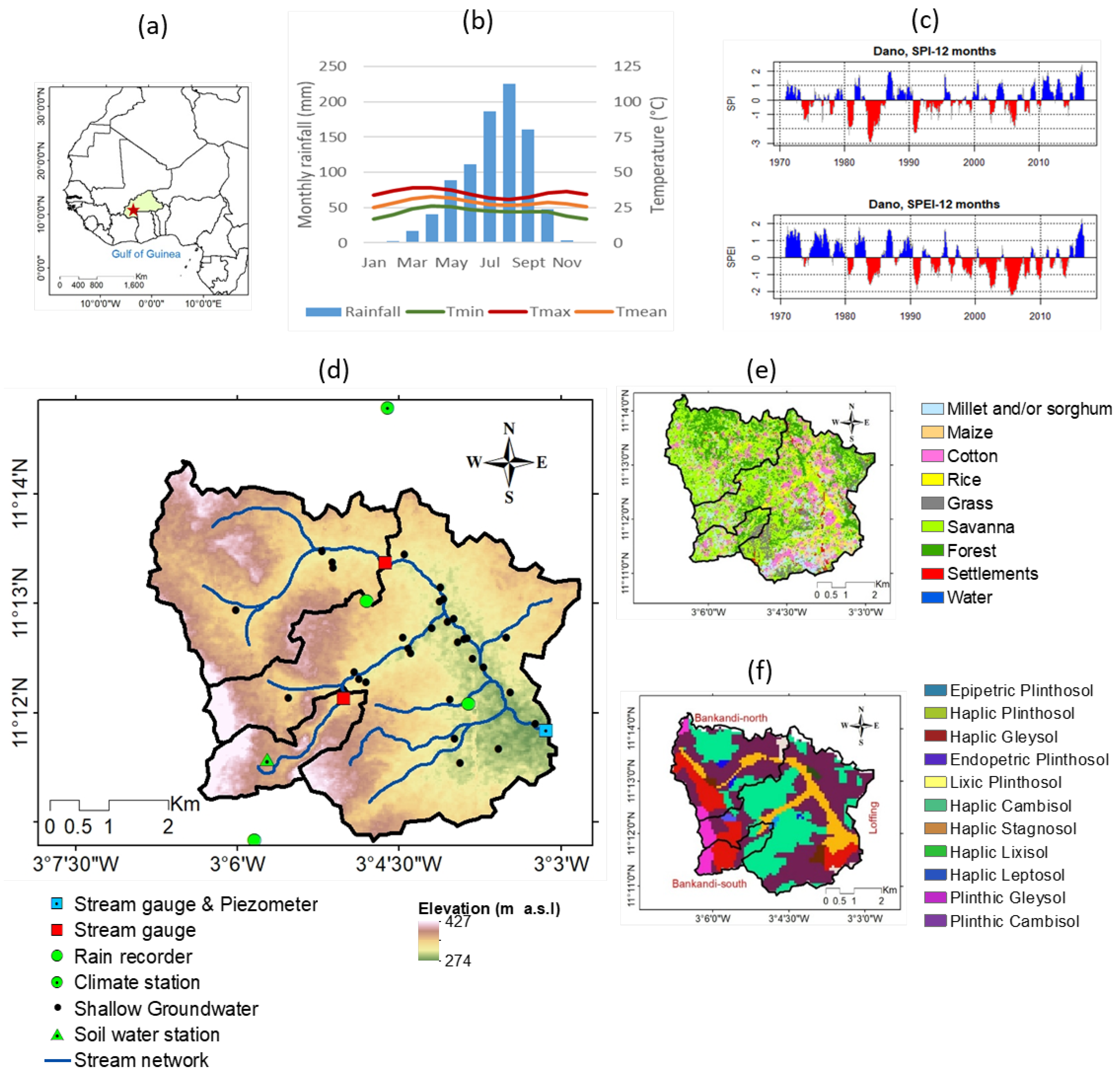
2.1. Study Area

The study area called Bankandi-Loffing is an inland valley catchment of 30 km² located in the south-west of Burkina Faso in West Africa (Figure 1). Except for the western border, comprising the Ioba Mountains, the majority of the catchment is characterized by flat terrain with a mean slope of 4° and a modal slope of 3°. This has allowed for the formation of inland valleys.

The climate is Sudan-Sahelian and is characterized by unimodal rainfall starting from May and ending in October, with a maximum rainfall in August (Figure 1b). The annual rainfall range is from 800 to 1200 mm with more than 2000 mm of potential evapotranspiration per year. The average daily temperature is 21–32 °C. The region experiences frequent occurrence of droughts (Figure 1c).

The geology of the catchment consists of Precambrian formations that are part of the West African craton. The Paleoproterozoic basement is made of Birimian green stone belts (from 2238 to 2170 million years old), volcano–sedimentary, and plutonic sequences [48]. The Ante-Birimian granites are found in upstream areas, and Birimian shists are located in the downstream areas of the catchment [49].

According to the soil classification of the World Reference Base [50], Plinthosols are the predominant soil types in the investigated area (Figure 1f). They cover 73% of the catchment area. Cambisols and Gleysols are the second most observed soil types in the area. Cambisols and Gleysols each account for 11% of the Bankandi-Loffing catchment. The texture of Plinthosols varies with soil depth from loam to clay, whereas the texture of Gleysols and Cambisols changes from clay loam or silt loam to silt clay loam. Plinthosols are frequently observed in uplands of inland valleys, while Gleysols and Cambisols are located in the valley bottoms.

The vegetation is mainly of the savanna type (a mix of shrubs, trees, and herbs) (Figure 1e). The savanna covers 40% of the Bankandi-Loffing catchment, while forest represents 20% of the catchment area. The most cultivated food crops are millet (Panicum miliaceum), sorghum (Sorghum bicolor), and maize (Zea mays). Millet and sorghum are cultivated in 11% of the catchment area, and 8% of the catchment are used for maize cultivation. Rice (Oryza sativa or Oryza glaberrima) is mainly cultivated in the valley bottoms of the inland valleys and is grown in 3% of the catchment area. Cotton is the major cash crop and accounts for 11% of the catchment area. Grasslands (5% of the catchment area) are used for cattle grazing.

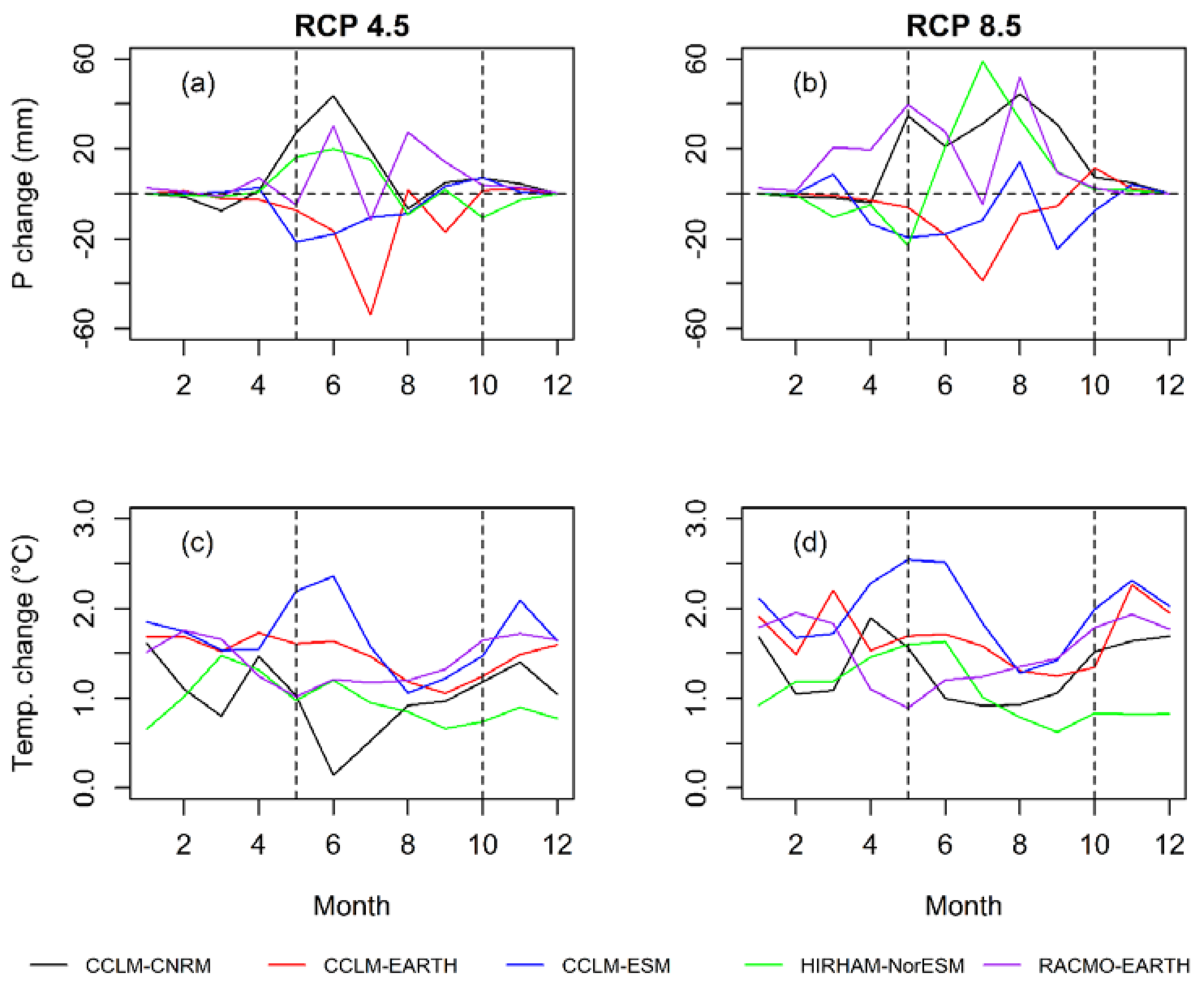
2.2. Climate Model Ensemble

The impact of climate change on water resources in an inland valley catchment was assessed using climate data of CORDEX-Africa. A climate ensemble constituting five RCM–GCMs was applied for the impact assessment (

Table 1. RCM–GCM products and the research centers of their production.

RCM–GCM Label	RCM	Driving GCM	RCM Center/Institute	Country of RCM Center/Institute	Acronym (Yira et al. [17])
M1	CCLM48	CNRM-CM5	CCLMcom	Germany	CCLM-CNRM
M2	CCLM48	EC-EARTH	CCLMcom	Germany	CCLM-EARTH
M3	CCLM48	ESM-LR	CCLMcom	Germany	CCLM-ESM
M4	HIRHAM5	NorESM1-M	DMI	Denmark	HIRHAM-NorESM
M5	RACMO22	EC-EARTH	KNMI	Netherlands	RACMO-EARTH

RCM: regional climate model; GCM: global climate model; CCLM: Climate Limited Modelling Community; DMI: Danish Meteorological Institute; KNMI: Royal Netherlands Meteorological Institute.

).

The ensemble was obtained from three regional climate models (RCMs) that use four global climate models (GCMs) as boundary conditions. An ensemble of several RCM–GCMs was necessary in order to account for the uncertainties associated with climate models [53,54]. An study at the regional scale by Laux et al. [40] recommended an ensemble of more than ten RCM–GCMs for precipitation-related impact studies. Due to data availability, the authors of the present study applied five RCM–GCMs. Each RCM–GCM datum consisted of precipitation and air temperature for a reference period (1971–2000) and a predicted period (2021–2050). According to Vautard et al. [55], the selected reference period corresponded to 0.46 °C air temperature increase compared to the pre-industrial period (1881–1910). For the predicted period, two greenhouse gas emission scenarios were considered, namely the representative concentration pathways (RCPs) 4.5 and 8.5 [56]. The daily temperature and precipitation of the RCM–GCMs were available at a 0.44° spatial resolution. Temperature and precipitation were extracted from 3 × 2 nodes, and the average values were applied to calibrate the WaSiM (Water flow and balance Simulation Model) hydrological model. Bias-corrected temperature obtained using the delta change approach [57] and precipitation obtained using the non-parametric quantile mapping [58] were employed to force WaSiM. Non-bias-corrected effects on impact assessments have been extensively discussed in previous studies [17,59]. Therefore, they are not presented in this study.

The decision to use only bias-corrected climate variables was motivated by the fact that bias correction reduces inconsistencies and deviations; it restores the timing of rainy seasons and considerably minimizes inter-node deviations [17]. This subsequently leads to a more realistic seasonal distribution of precipitation and air temperature. Therefore, bias correction makes climate variables suitable for the hydrological impact assessment of climate change [15,17,25,59,60,61,62].

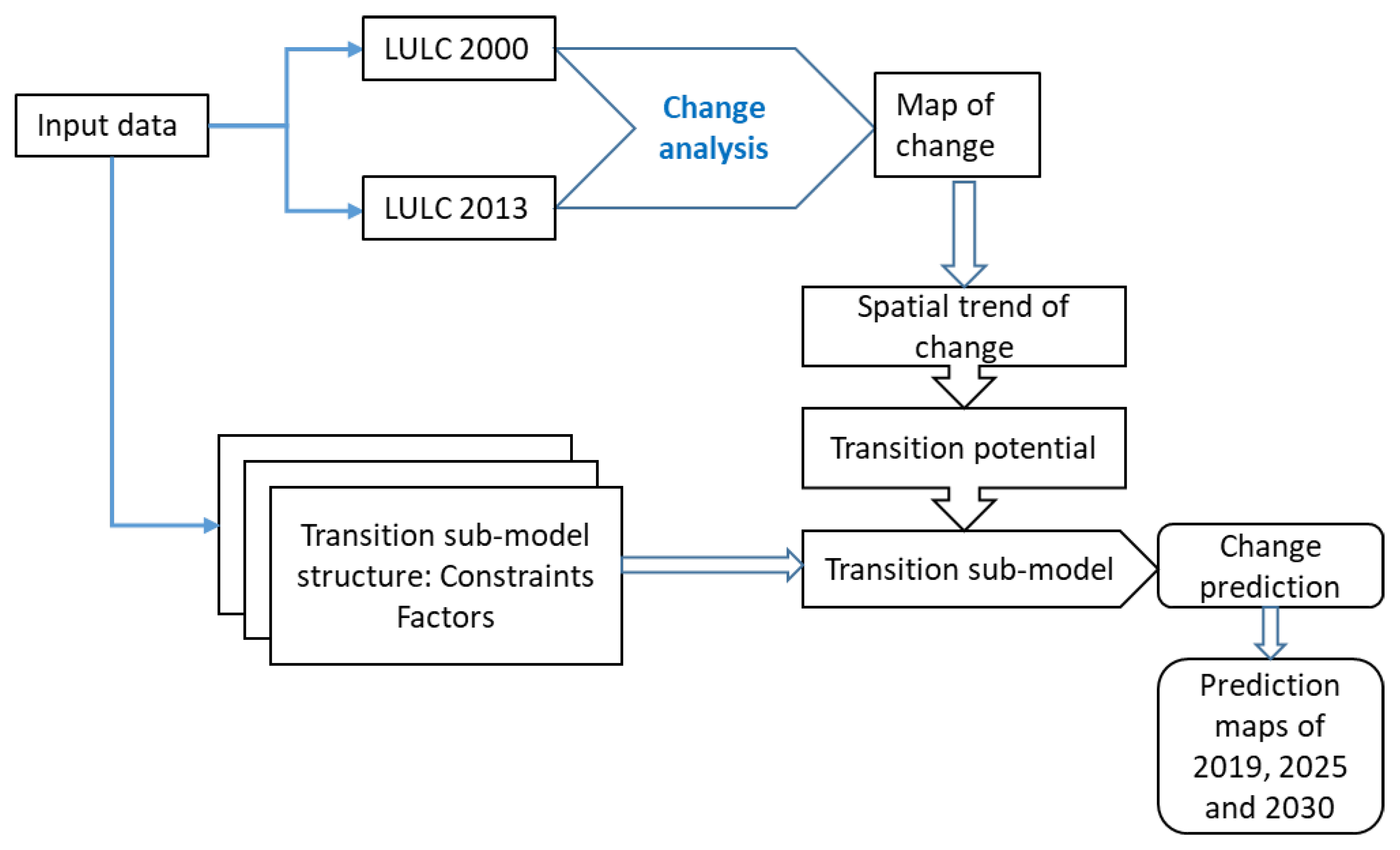
2.3. Land Use/Land Cover (LULC) Prediction

The historical LULC data were obtained from the work of Landmann et al. [63] and Forkuor [51]. Satellite images from three sensors, namely Landsat, RapidEye, and TerraSAR-X, were used. Only satellite images with a cloud coverage of less than 20% were considered for download. The catchment falls into tile Path 196, Row 052. The spatial resolution ranges from 5 to 30 m. The acquisition dates were in the cropping seasons in order to capture different crop-growing stages.

The future LULC maps (LULC-2019, LULC-2025, and LULC-2030) were developed based on historical maps (LULC-2000 and LULC-2013) using the Land Change Modeler (LCM) [64]. The LCM is an empirically driven processing software that follows three steps. The first step is the past land cover analysis, and the second step is the modelling of transition potentials. For this step, the LCM uses a multi-layer neural network [65] to model the potential for land transition from one land use class to another. The method considers multiple variables including slopes, distance to roads, previously deforested areas, and settlements. The calibrated transition potential model is then used for future scenario predictions. Finally, the last step consists of using historical rates of change and the transition potential model to determine changes of land use per pixel and time step. At this step, a stochastic Markov chain technique [66] is applied to simulate the probability of LULC, and a future LULC map is generated. The LCM is presented in Figure 2.

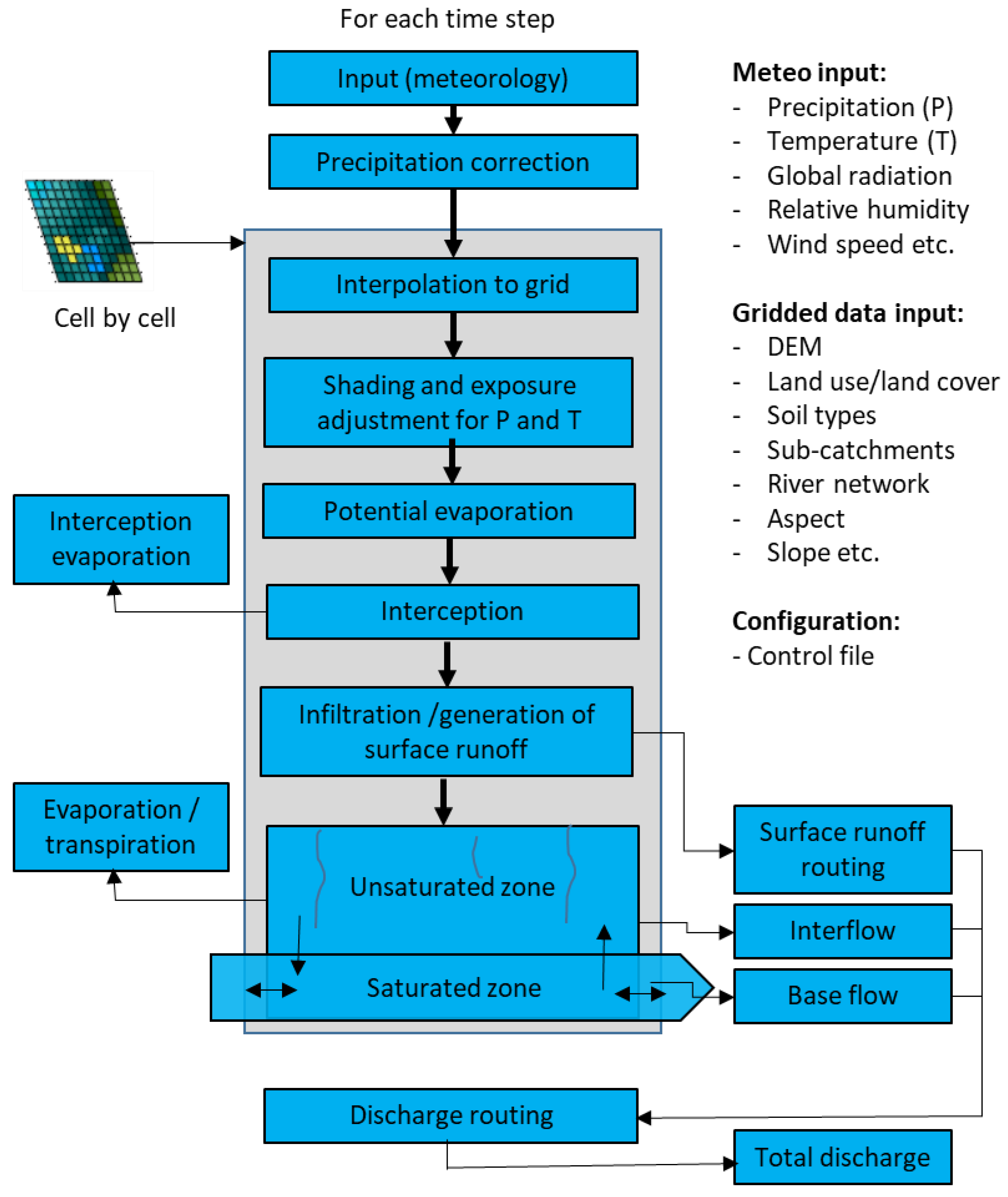
2.4. Calibration and Validation of the Hydrological Model

To study the impacts of climate change on hydrology, a calibrated hydrological model is often forced by RCM–GCM climate variables including precipitation and temperature [21,24,68,69,70,71]. In this study, the Water flow and balance Simulation Model (WaSiM) was applied (Figure 3).

The Bankandi-Loffing catchment was initially calibrated and validated at an hourly time step using the Penman–Monteith approach [73] for evapotranspiration estimation [74]. As temperature is the only climate variable available at a daily time step for evapotranspiration approximation, the model was recalibrated at a daily time step using the Hamon method to estimate evapotranspiration for the climate impact assessment [72,75,76,77]. The recalibration of the model was solely based on the optimization of the Hamon monthly correction factor, which depends on season and location. The model was calibrated during 2014–2015 and validated in 2016 using LULC-2013 as a reference, and the annual water balance was estimated.

2.5. Estimation of the Hydrological Model Performance

A multi-criteria approach was applied for model performance estimation in order to account for the deficiency of a single criterion approach [78]. The objective functions include the Nash–Sutcliffe Efficiency (NSE) [79], the Kling–Gupta Efficiency (KGE) [29,80], the coefficient of determination (R²) [81], and the percent bias (Pbias) [82]. The optimization of the model is oriented towards maximizing each of the first three objective functions (R², NSE, and KGE) for discharge with a perfect model yielding 1 for each of them. R² ranges from 0 to 1, whereas NSE and KGE range from −∞ to 1. Concerning Pbias, the optimal value is zero, and it ranges from −100% to +∞. The positive and negative Pbias are equivalent to overestimation underestimation, respectively, of the discharge by the model. A model is assessed as being satisfactory when NSE > 0.5 and −25% < Pbias < +25% [82]. A lower satisfactory limit of 0.5 is also considered for KGE.

The most optimal parameter set is assumed to be the one with the highest KGE for discharge. This is due to the fact that KGE not only incorporates R² in its equation but also accounts for both conditional and unconditional biases [80,83]. According to Equation (2), maximizing each of the components of KGE will result in maximizing KGE [29].

R² was not chosen to select the optimal simulation as it only measures the concentration of points around an imaginary line in a graph simulated against observed discharge. R² does not measure the concentration of points around a 1:1 line (R² is susceptible to systematic errors). The use of only R² for model performance estimation might be misleading [78].

Although NSE is the most employed dimensionless objective function in hydrological modeling, it has been criticized for using mean observed discharge as the baseline. This might lead to the overestimation of model performance when a significant seasonal variation of runoff is observed [80].

2.6. Climate and Land Use Scenarios

Climate and land use scenarios were implemented according to

Table 2. Model setup for the hydrological impact assessment of climate and land use.

	Reference		Prediction
Scenario	LULC	Historical RCM–GCM	LULC	RCM–GCM (RCP 4.5 and 8.5)
1	2013	1971–2000	2013	2021–2050
2	2013	1971–2000	2030	2021–2050

LULC: land use and land cover; RCM: regional climate model, GCM: global climate model; RCP: representative concentration pathway.

. For each of the five RCM–GCMs, the bias-corrected precipitation and temperature were utilized as input for the calibrated hydrological model. The hydrological model was separately run for each of the three components of the RCM–GCM (reference period, RCP 4.5, and RCP 8.5) for 30 years. The reference period (1971–2000) and the predicted period (2021–2050) were preceded by the same warmup period of 6 years. The water balance of each RCM–GCM for RCP 4.5 and RCP 8.5 were compared to their counterpart reference periods. An equal duration (30 years) of predicted and reference periods was used, and the predicted periods were compared to the reference period in order to cancel out systematic bias related to the hydrological and climate models. The systematic error is assumed to be constant between the reference period and the predicted period [84]. The identical warmup period was used to avoid variation in the initial conditions of the hydrological model.

The predicted RCM–GCMs were compared to their counterpart modeled past and not to the observed historical data because the bias correction was not perfect. Therefore, comparing predicted modeled data with observed data could add a new layer of uncertainty to the impact assessment.

LULC-2013 was considered as the reference LULC and was used during the reference period and the predicted periods, except while assessing the combined climate and land use change impact. During the assessment of combined climate and land use change impact, LULC-2013 was replaced by LULC-2030 for the predicted future climate scenarios (Table 2).

3. Results and Discussion

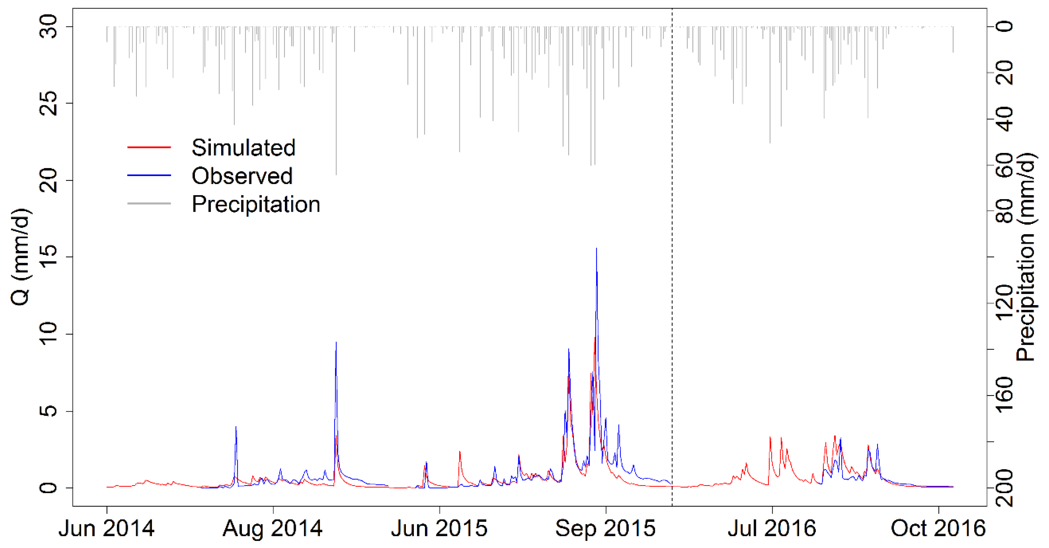
3.1. Hydrological Model Performance and Water Balance

The simulated hydrograph (Figure 4) and the model performance statistics (

Table 3. Mean annual water balance and the model performance.

	Calibration (2014–2015)	Validation (2016)	Annual Mean (2014–2016)
P (mm)	1067	1001	1045
ETa (mm)	982	954	973
Qt (mm)	96	113	102
Qs (mm)	39	46	41
Qi (mm)	40	43	41
Qb (mm)	18	23	19
Delta S (mm)	−11	−66	−30
R²	0.59	0.71	-
NSE	0.57	0.48	-
KGE	0.66	0.73	-
Pbias (%)	−23.70	21.20	-

P: precipitation; ETa: total actual evapotranspiration; Qt: total runoff; Qs: surface runoff; Qi: interflow; Qb: base flow; Delta S: change in storage; R²: coefficient of determination; NSE: Nash–Sutcliffe Efficiency; KGE: Kling–Gupta Efficiency.

) demonstrated a good performance of the hydrological model at the daily time step using the Hamon method for evapotranspiration estimation. There was good agreement between simulated and observed total runoff in terms of timing and magnitude. Most of the peak flows were well-captured. However, some extreme events were not well-captured. This can be attributed to the uncertainty increase in the observed data with the size of the flood due to overbank flows.

The Kling–Gupta efficiency (KGE) [29,80] was approximately 0.7 for the calibration and validation periods. The Nash–Sutcliffe efficiency (NSE) [79] (≥0.5) and percent bias (24% for calibration period and 21% for validation) were satisfactory [82,85].

The annual average change in storage was negative during the simulation period (delta S = −30 mm). This is partly attributed to not only the short simulation period but also (mainly) to the high inter-annual variability of rainfall during the observation period (2014–2016). The annual rainfall in the year 2015 was 21% higher than that of the year 2014 and 16% higher than that of the year 2016. Therefore, the simulation period could not be qualified as a stationary period and the equilibrium of the water balance was not completely reached. In the dry years, the water deficit was compensated for by the soil moisture originating from the shallow groundwater of inland valley bottoms. In the valley bottoms, the groundwater table was found to be near the ground surface and consequently significantly contributes to soil moisture through capillary action.

In general, the water balance was found to be in the range of previous studies in the region [17,42,86]. Given that the impact assessment was conducted by comparing the modeled relative alterations in water balance components between the predicted period and the simulated reference period, the systematic error was cancelled out [87].

3.2. Predicted Land Use Land Cover

Figure 5 shows a gradual conversion of savanna to cropland and settlement. The average annual reduction rate of savanna was 1.1% of the catchment area, and the highest conversion rate occurred from 2007 to 2013 (3.3% of the catchment area per year). The trend of savanna conversion was previously reported by Yira et al. [42], who analyzed the impact of LULC change on hydrological processes in the catchment including evapotranspiration and soil infiltration. The change in evapotranspiration could be attributed to the change in vegetation characteristics such as albedo, which modifies evapotranspiration by changing net solar radiation [73]. In addition to albedo, canopy surface resistance, leave area index, root depth, and the length of the growing period are influenced by LULC change and consequently led to variations in evapotranspiration.

However, LULC change influences infiltration rates by modifying macropore distribution in the soil. In a similar catchment in Northern Benin, Giertz et al. [43] demonstrated a significant decrease in the number of macropores from savanna to cropland. Macropore distribution was found to affect interflow and base flow.

On the question of drivers of land use change, many studies have suggested that population growth in West Africa (3% per year) is the main driver of savanna conversion to cropland [42,47,88,89,90,91]. This is needed to satisfy the considerable increase in food demand in the region. Moreover, the evolution of the farming systems suggests that the development of cotton cultivation has significantly contributed to the savanna conversion [42,47]. The production of cotton increased from 75,476 t in 1990 to 280,000 t in 2013 (270% increase) at the country level [92].

Other drivers of natural vegetation conversion into croplands include bushfires, mining, wood harvesting, and climate variability [93]. The conversion is frequently associated with the vulnerability of soil to erosion and soil fertility losses. This, in return, exacerbates more natural ecosystem conversion to agriculture. Hounkpatin et al. [94] estimated soil organic carbon loss in the Dano catchment of up to 24 t C ha⁻¹ (ton carbon per hectare) at the top 10 cm and 49 t C ha⁻¹ at the upper 30 cm in 29 years.

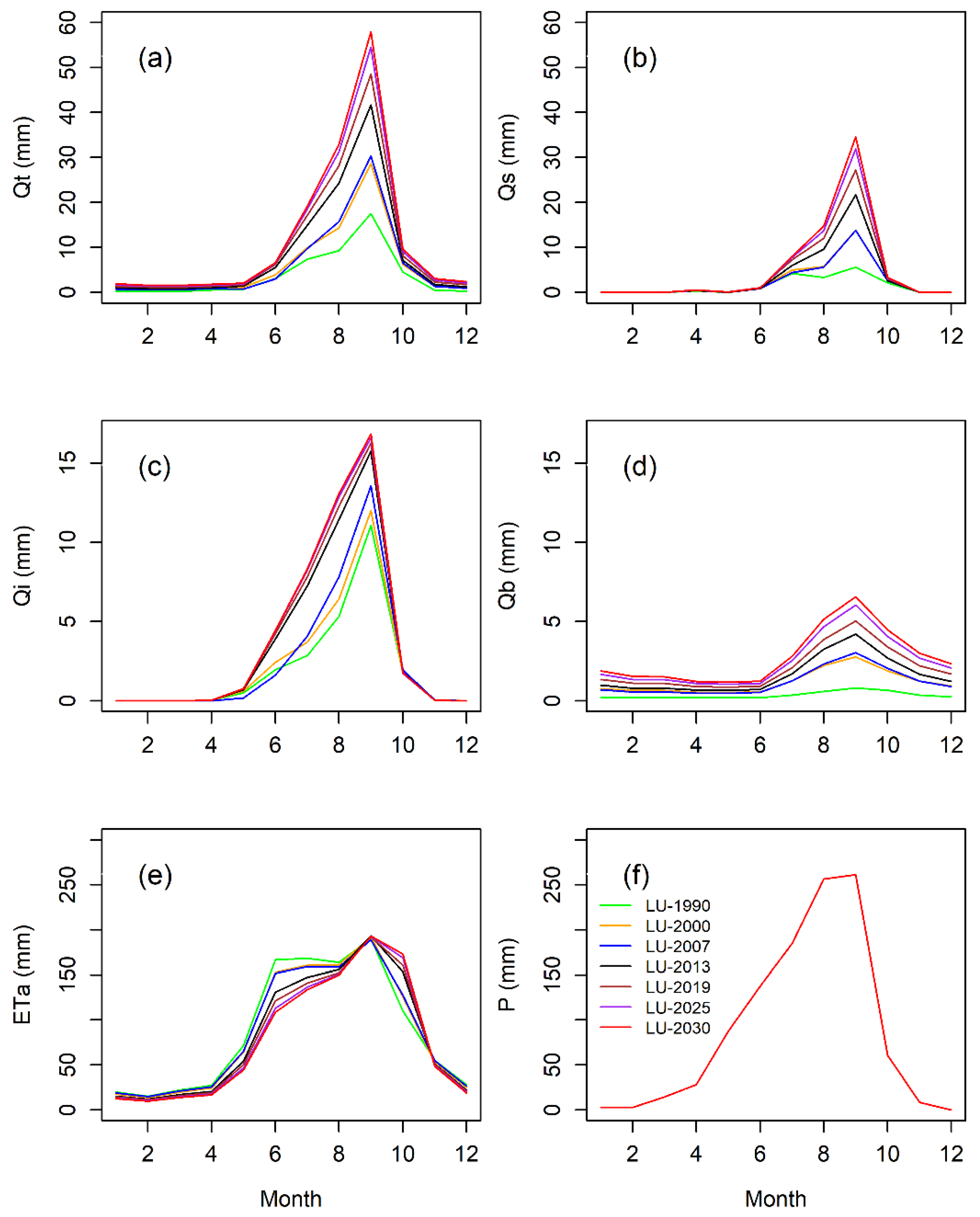
3.3. Sensitivity of the Hydrological Model to LULC Change

Four historical LULC maps (LU-1990, LU-2000, LU-2007, and LU-2013) and three predicted future LULC maps (LU-2019, LU-2025, and LU-2030) were utilized to run the calibrated hydrological model for three years (2014–2016). The annual mean water balance results (

Table 4. Mean annual water balance for each land use land cover for the period of 2014–2016.

	Land Use and Land Cover
	LU-1990	LU-2000	LU-2007	LU-2013	LU-2019	LU-2025	LU-2030
P (mm)	1045	1045	1045	1045	1045	1045	1045
ETa (mm)	1039	1011	1014	973	950	934	924
Qt (mm)	44	69	71	102	119	133	140
Qs (mm)	16	28	27	41	51	58	62
Qi (mm)	24	27	29	41	43	45	45
Qb (mm)	4	14	14	19	25	30	33

LU: land use and land cover; P: precipitation; ETa: total actual evapotranspiration; Qt: total runoff; Qs: surface runoff; Qi: interflow; Qb: base flow; Cr: simulated total runoff coefficient.

) demonstrated a linear decrease in the actual evapotranspiration (ETa), while the total runoff increases with conversion of savanna to croplands. The savanna area decrease was found to be highly correlated to the change in mean annual ETa, and more than 96% of the variation of the annual ETa could be attributed to the decrease in savanna area (Pearson correlation coefficient R² = 0.96; p-value = 0.0001). The relative decrease in ETa from LU-2013 to LU-2030 was −5%, whereas the relative increase in the total runoff was +27%. This seems to suggest that runoff was nearly six times more sensitive to savanna conversion than ETa. Moreover, the increase in the total runoff was primarily driven by the increase in the surface runoff (R² = 0.996; p-value < 0.0001). This could contribute to a soil erosion increase and a soil fertility loss for agriculture [95].

The variation of average monthly ETa (Figure 6e) suggested that the largest differences between the land use scenarios occurred at the beginning (May, June, and July) and the end of the rainy season (October). The magnitude of monthly ETa in September was approximately the same for all the land use scenarios. This can be explained by the fact that there was sufficient water to satisfy the monthly potential evapotranspiration in September. The total runoff (Figure 6a), surface runoff (Figure 6b), and base flow (Figure 6d) clearly demonstrated September as the month of the highest contrast between the scenarios, while August recorded the maximum variance for interflow (Figure 6c).

Many authors have documented the conversion of savanna to cropland in the region and a subsequent increase in runoff [42,47,91,93,96,97,98,99]. Mahé et al. [99] reported 30% decline in natural vegetation and 23% cropland increase from 1965 to 1995 in the Nakambe River basin in Central–Northern Burkina Faso. They attributed the subsequent increase in runoff to the decrease in soil water holding capacity (WHC). In a similar climatic zone in Northern Benin, Giertz et al. [43] found that the infiltration rate of natural savanna was significantly higher than that of croplands. Therefore, croplands tend to produce more runoff than savanna areas.

It is noteworthy that evapotranspiration was found to considerably influence the outcome of the resulting water balance in this study. None of soil parameters were modified. Thus, the change in water balance could not be attributed to a change in infiltration. As the Hamon method of evapotranspiration was applied instead of the Penman–Monteith method, parameters such as albedo and canopy surface resistance could not explain the variation of the actual evapotranspiration either [73,75]. The major parameter in this study that was found to influence the change of the water balance with land use change was root depth, which was influenced by the length of vegetation period. The root depth varied throughout the year from 0.2 to 1.8 m under the natural savanna. Most of cropland comprised bare soil (root depth 0 m) during the dry season (January to May). In the cropping period (from June to October), the root depth ranged from 0.01 to 0.53 m. The following parameters may have contributed to a lesser extent: the specific thickness of water layer on the leaves (interception parameter, IntercepCap), the root distribution (RootDistr), the vegetation cover fraction (VCF), and the leave area index (LAI). This is supported by the results of Leemhuis et al. [100] and Beck et al. [101] in their studies in tropical regions in Indonesia and Puerto Rico, respectively. Hence, evapotranspiration reduction as a result of natural savanna conversion to cropland favors infiltration excess runoff by increasing soil moisture. Furthermore, it is important to note that rainfall characteristics (intensity and distribution in time) play crucial roles in runoff generation [102,103].

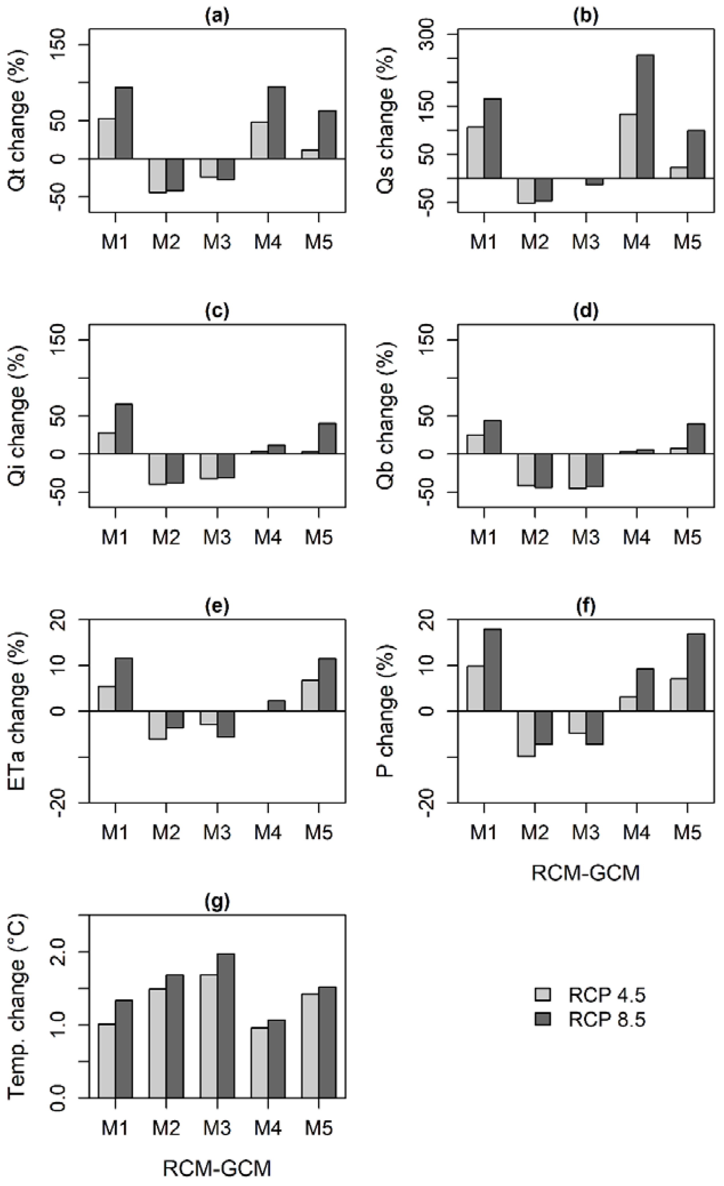
3.4. Climate Change Impact on Hydrological Response

Figure 7 illustrates the input climate model data (precipitation and air temperature) and the output main water balance components (total runoff, surface runoff, interflow, base flow, and actual evapotranspiration) for the reference period (1971–2000). The comparison between the five RCM–GCMs using the nonparametric, pairwise, and corrected Wilcoxon test showed no significant difference for the reference climate input data of most of the RCM–GCMs. This suggests that most of the RCM–GCMs belonged to the same population and had a similar distribution for the reference period. However, significant differences were observed in the actual evapotranspiration between RACMO-EARTH and each of the following models: CCLM-CNRM (p-value = 0.0197), CCLM-ESM (p-value = 0.0164), and HIRHAM-NorESM (p-value = 0.0426). A similar result was observed for base flow with significant differences between RACMO-EARTH and CCLM-CNRM (p-value = 0.0309) and between RACMO-EARTH and CCLM-ESM (p-value = 0.0426). It is important to note that a significant difference for base flow occurred, although there was no significant difference for the total runoff was due to the low contribution of base flow to runoff.

The relative changes in temperature and precipitation and the implication for water balance components are depicted in Figure 8. All models revealed an increase in temperature compared to the reference period (Figure 8g). The increase in temperature is higher for RCP 8.5 than RCP 4.5. This is because the greenhouse forcing of RCP 8.5 (>1370 ppm CO₂ equivalent) is stronger than the greenhouse forcing of RCP 4.5 (~650 ppm CO₂ equivalent) [56]. The annual increase in temperature was found to range from 1 to 2 °C until 2030. The highest increases in temperature were predicted by CCLM-EARTH and CCLM-ESM. The predicted temperature was consistent with the decision adopted by the Conference of the Parties at its twenty-first session in Paris (COP 21). The Paris agreement urgently recommended that parties limit the temperature increase to well below 2 °C compared to the pre-industrial level [54,104,105].

Although the investigated climate models unanimously simulated an increase in temperature, they diverged on precipitation signals (Figure 8f) and the uncertainties were high among the ensemble members. CCLM-EARTH and CCLM-ESM predicted the highest increases in temperature and projected negative precipitation signals, while the other models (CCLM-CNRM, HIRHAM-NorESM, and RACMO-EARTH) simulated positive signals. For the models that predicted positive precipitation signals, the increase in annual precipitation was higher under high greenhouse gas forcing (RCP 8.5) than moderate greenhouse gas forcing (RCP 4.5). However, for the models that predicted negative precipitation signals, there was no clear trend of precipitation signals as function of greenhouse gas concentration. The climate models predicted precipitation increases from 3% (predicted by HIRHAM-NorESM under RCP 4.5) to 18% (predicted by CCLM-CNRM/RCP 8.5), and the decreases ranged from −10 to −5%. Yira et al. [17] obtained an increase from +1 to +18% and a decrease from −9 to −6% in precipitation in a 6.5-times larger catchment in Dano compared to the Bankandi-Loffing catchment. Op de Hipt et al. [59] found an increase from +6 to +19% and a decrease from −11 to −4% in the Dano catchment (4 times larger than the Bankandi-Loffing catchment). It is noteworthy that the selected climate models did not present opposite signals between RCP 4.5 and RCP 8.5.

Furthermore, the models with higher increases in temperature projected lower increase in mean annual precipitation, whereas the models with lower increases in temperature showed higher increases in mean annual precipitation. This seems to contradict the Clausius–Clapeyron relation [106]. According to the Clausius–Clapeyron equation, rainfall intensity increases with greenhouse gas under constant moisture availability at global or regional scale. Annual comparison of rainfall in this study might be the reason for the differences. Additionally, at a local scale, air moisture might significantly vary. Importantly, the distribution of daily rainfall showed an increase in the 95th percentile for most of the models. The daily rainfall 95th percentile increased in a range from 2% to 24% compared to the reference period for all the models. This was applicable to the negative and positive precipitation signal models. The increase in intense rainy days was associated with a decrease in rainy days for most of the climate models. This is consistent with previous studies in the region that demonstrated not only an increased rainfall intensity and a decreased number rainy days but also a delay of rainy season onset [7].

The direction of change in the estimated water balance components (Figure 8a–e) were superimposed by precipitation signals. CCLM-EARTH and CCLM-ESM showed negative changes, while the other models predicted positive changes. This suggests that the predicted water balance was mainly influenced by precipitation in the study area. This is consistent with the work of Yira et al. [17], who found that this is attributed to water-limited conditions of the area. Evidence from a similar catchment in California simulated using the SWAT model is also in line with these findings [107,108]. However, insight from Op de Hipt et al. [59] seems to indicate that potential evapotranspiration is more influential on runoff than rainfall; they attributed the divergent finding to the structural difference between the hydrological models SHETRAN [109] and WASIM [72].

The annual actual evapotranspiration (ETa) (Figure 8e) was found to vary from 0% (no change) predicted by HIRHAM-NorESM/RCP 4.5 to +12% projected by CCLM-CNRM/RCP 8.5. CCLM-EARTH/RCP 4.5 projected the lowest ETa decrease (−6%). In contrast with ETa, the total runoff (Figure 8a) exhibited a much higher increase (from +12% to +95%) and decrease (from −44% to −24%). The total runoff decrease was expected to be an order of magnitude less than the increase but still more prominent than the decrease in ETa.

A more detailed analysis of the runoff components clearly demonstrated that surface runoff (Figure 8b) was expected to have a major change. The maximum surface runoff change was predicted by HIRHAM/RCP 8.5 (+256%), followed by CCLM-CNRM/RCP8.5 (+166%). Moreover, a considerable increase in surface runoff was noted under RCP 4.5, such as a +133% increase projected by HIRHAM-NorESM and a +106% increase by CCLM-CNRM. However, CCLM-EARTH predicted decreases of −51% and −46% under RCP 4.5 and RCP 8.5, respectively, and CCLM-ESM projected negligible change in surface runoff under RCP 4.5 and an only −12% decrease under RCP 8.5. If the increase in surface runoff, such as that predicted by CCLM-CNRM and HIRHAM-NorESM, occurred, it would be detrimental for soil in terms of erosion and fertility loss [42,47,59,95,110].

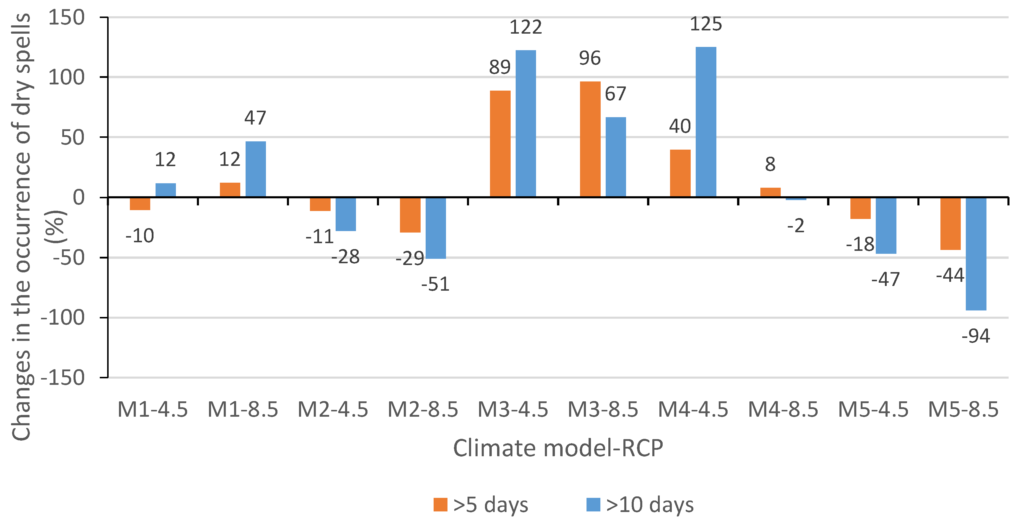
3.5. Predicted Dry Spell Change

Daily bias-corrected modelled rainfall data were utilized to analyze dry spells of >5 days and >10 days in wet seasons (from June to October) by comparing the predicted period (from 2021 to 2030) with the reference period (from 1971 to 2000). The threshold of a rainy day was assumed to be 0.1 mm.

Figure 9 depicts the variable relative change of dry spells for the five climate models under RCP 4.5 and RCP 8.5. Some models predicted increases in dry spells. The increase in dry spells ranged from 12% to 96% for >5 day dry spells and from 12% to 125% for >10 day dry spells compared to the reference period. Nonetheless, other models projected a decrease in dry spells that ranged from −10% to −44% for >5 day dry spells and from −2% to −44% for >10 day dry spells. The models CCLM-EARTH and CCLM-ESM predicted a decrease in annual rainfall (Figure 8f). However, CCLM-EARTH predicted a decrease in dry spells, whereas CCLM-ESM predicted an increase in dry spells. This suggests that the decrease in annual rainfall was mainly due to an increase in dry spells for CCLM-ESM. This is in line with the work of Kendon et al. [111], who found the decrease in precipitations to be due to decrease in rainfall occurrence in the West African region. As for CCLM-EARTH, the decrease in annual rainfall might have been due to its projection of light rainfall. However, some models have been reported to show increase sin rainfall intensity in the region [112].

In general, the changes in >10 day dry spells were expected to be higher than the changes in >5 day dry spells. In a similar study in East Africa, it was found that maize experienced at least one >10 day dry spells in a range from 74% to 80% of the season [113]. The occurrence of dry spells during the flowering and grain filling stages might lead to yield reduction or crop failure [114,115].

3.6. Climate and Land Use Change Impact on Hydrology

The results of the combined impact of climate and land use change on hydrology are depicted in Figure 10. The land use change exacerbated the increase in runoff due to climate change (Figure 10a). Under the effect of land use 2030, CCLM-CNRM, HIRHAM-NorESM, and RACMO-EARTH projected a total runoff increase range from +52% to +158% compared to the reference period. The maximum increase was predicted by CCLM-CNRM/RCP 8.5, whereas the lowest increase was observed with RACMO-EARTH/RCP 4.5. Total runoff increased by a factor of 1.4–4.5 times compared to the climate change impact only scenario depending on the ensemble member.

Nevertheless, the CCLM-EARTH and CCLM-ESM models predicted a total runoff decrease range from −29% to −11%. In this case, the highest and the lowest decrease were observed under RCP 4.5 forcing. Land use change reduced the impact of climate change for these climate models (CCLM-EARTH and CCLM-ESM) by a factor of 0.5–0.7 compared to the climate change impact only scenario.

A comparison with the previous scenario (climate change impact only) clearly revealed that from 27% to 78% of total runoff change could be attributed to land use change. Consequently, the impact of land use change on the total runoff significantly varied with the climate model. The maximum land use change contribution was predicted under RACMO-EARTH/RCP 4.5 forcing, whereas the minimum land use change impact contribution was projected under HIRHAM-NorESM/RCP 8.5. Thus, the projected land use impact indicated that the impact of land use change on total runoff is not negligible and cannot be ignored when studying future climate impact on hydrology in the area.

The runoff component analyses (Figure 10b–d) revealed that the major driver of runoff change was surface runoff (Figure 10b). A nearly fourfold increase in surface runoff was expected under RCP 8.5 for CCLM-CNRM (+281%) and HIRHAM-NorESM (+305%). Surface runoff was projected to approximately triple under RACMO-EARTH/RCP 8.5 (+186%), CCLM-CNRM/RCP 4.5 (+185%), and HIRHAM-NorESM/RCP 4.5 (+173%). This could subsequently intensify soil erosion, with disastrous loss in soil fertility if no mitigation strategies are put in place.

It is interesting to note a significant increase in base flow with land use change from 3–44% in the first scenario (Figure 8d) to 67–141% (Figure 10d) in the second scenario compared to the reference period. The contribution of the land use change to base flow increase was therefore estimated to be 69–96% of the combined land use and climate change. This seems to suggest that land use change is the major driver of base flow change in the catchment. No direct relationship existed between base flow and land use parameters. The increase in the base flow with land use change can be attributed to the surplus of water due to the decrease in ETa from the first scenario (from 0% to 12% compared to the reference period; Figure 8e) to the second scenario (from −3% to 7% compared to the reference period; Figure 10e). This may be attributed to the fact that root depth was greater in the savanna (from 0.2 to 1.8 m used for WaSiM parameterization) than in croplands (from 0 to 0.61 m used for WaSiM parameterization).

The monthly signal variations of the input climate variables (Figure 11) and the subsequent simulated water balance before and after the application of land use change (Figure 12) illustrated the seasonal variations of the water balance (in mm).

Figure 11a,b suggests that the peak rainfall changes occurred in June under RCP 4.5 for CCLM-CNRM, HIRHAM-NorESM, and RACMO-EARTH, whereas the peaks were expected two months later (in August) under RCP 8.5 for CCLM-CNRM and RACMO-EARTH. The peak magnitude of rainfall change increased from RCP 4.5 to RCP 8.5 for CCLM-CNRM, HIRHAM-NorESM, and RACMO-EARTH (positive precipitation signal models) and decreased from RCP 4.5 to RCP 8.5 for CCLM-EARTH (negative precipitation signal model).

The simulated monthly change in total runoff is depicted by Figure 12(a1–a4). Like rainfall, the extreme changes of total runoff under RCP 8.5 forcing were delayed compared to those under RCP 4.5 forcing. For instance, the extreme changes of total discharge were expected in July under RCP 4.5 forcing, whereas they were expected in August under RCP 8.5 for CCLM-CNRM, HIRHAM-NorESM, and CCLM-EARTH. A similar prediction was obtained for surface runoff (Figure 12(b1–b4)) and interflow (Figure 12(c1–c4)). However, base flow peak changes were projected to occur in August regardless of greenhouse gas forcing.

For ETa, no general trend could be observed in terms of the time of occurrence of the peaks for the first scenario (Figure 12(e1,e2)). However, under the second scenario (Figure 12(e3,e4)), the ETa change appeared to gradually increase during the rainy season from June to October.

4. Conclusions

The hydrological impacts of climate and land use change were investigated in an inland valley catchment using five RCM–GCMs under RCP 4.5 and RCP 8.5 greenhouse gas forcing. After the calibration and validation of WaSiM, bias-corrected simulated daily rainfall and temperature were applied to force the hydrological model for the reference period (1971–2000) and the future period (2021–2050).

The calibration (2014–2015) and validation (2016) of the WaSiM presented good agreement in terms of hydrographs and objective functions between the observed and simulated discharge. KGE was equal to approximately 0.7, NSE > 0.5, and Pbias ranged between 21% and 24%.

The sensitivity of the hydrological model to land use change was investigated using four historical LULC maps from 1990 to 2013 and three simulated LULC maps from 2019 to 2030. The results showed an increase in runoff over time with the conversion of the savanna to croplands.

The impact of climate change on streamflow was assessed by comparing the predicted period with the reference period. The results suggested a large spread for the future change of runoff in response to the non-agreement between the RCM–GCM simulations. Three models projected an increase in the total runoff from +12% to +95% and ETa from 0 to 12%, whereas two models predict decreases in total runoff from −44% to −24% and ETa from −6% to −3%. Surface runoff was projected to record the highest relative change compared to the other runoff components.

The combined climate and land use change was estimated by using LULC-2013 in the reference period and LULC-2030 as future land use. The results indicated that land use change exacerbated the increase in total runoff (from +52% to +158% compared to the reference period) predicted by the three RCM–GCMs and reduced the decrease in total runoff (from −29% to 11% compared to the reference period) predicted by the other two models.

After comparing the two scenarios, it was concluded that the contribution of land use change impact on hydrology was substantial and significantly varied with the climate model (from 27% to 78% of the combined climate and land use change).

The spread of the future predictions did not lead to one direction to follow for the development of climate adaptation strategies. However, the selected model ensemble allows for the exploration of both directions of change (increase or decrease in water resource). Given the uncertainty of the future projections and the adverse impacts that might arise from the implementation of some adaptation strategies, it is clearly better to opt for preventive measures.

The results of this study can be used as input to water management models in order to derive strategies to cope with present and future water scarcities for smallholder farming in the investigated area. The adaptation measures could include:

• The building of stone-lines, mulching, and agroforestry to reduce excess runoff and increase soil water availability (as options to react on increasing surface runoff).
• The creation of infiltration facilities (wells, ponds, artificial wetlands, and check dams) to reduce direct evaporation and increase groundwater storage.
• The introduction of short-time growing crops in order to cope with increased dry spells.

Combining short- and long-term hydrological information could help smallholder farmers who generally practice rainfed agriculture to make informed decisions regarding how to cope with the adverse impacts of climate change. Unfolding that potential can be facilitated by conveying the information on the current hydro-meteorological situation (in relation to deviation from long-term situation) on short-notice to smallholders via extension service and digital channels.

References

1. AGRA—Alliance for Green Revolution in Africa. Africa Agriculture Status Report 2016—Progress towards Agricultural Transformation in Africa; AGRA: Nairobi, Kenya, 2014. [Google Scholar]
2. Jalloh, A.; Nelson, G.C.; Thomas, T.S.; Zougmoré, R.; Roy-macauley, H. West African Agriculture and Climate Change: A Comprehensive Analysis; International Food Policy Research Institute: Washington, DC, USA, 2013. [Google Scholar] [CrossRef]
3. FAO. The FAO Statistical Yearbook 2014: Africa Food and Agriculture; FAO: Accra, Ghana, 2014. [Google Scholar]
4. Hollinger, F.; Staatz, J.M. Agricultural Growth in West Africa: Market and Policy Drivers; Food and Agriculture Organization and African Development Bank: Rome, Italy, 2015. [Google Scholar]
5. Mougin, E.; Hiernaux, P.; Kergoat, L.; Grippa, M.; de Rosnay, P.; Timouk, F.; Le Dantec, V.; Demarez, V.; Lavenu, F.; Arjounin, M. The AMMA-CATCH Gourma Observatory Site in Mali: Relating Climatic Variations to Changes in Vegetation, Surface Hydrology, Fluxes and Natural Resources. J. Hydrol. 2009, 375, 14–33. [Google Scholar] [CrossRef] [Green Version]
6. Lebel, T.; Cappelaere, B.; Galle, S.; Hanan, N.; Kergoat, L.; Levis, S.; Vieux, B.; Descroix, L.; Gosset, M.; Mougin, E. AMMA-CATCH Studies in the Sahelian Region of West-Africa: An Overview. J. Hydrol. 2009, 375, 3–13. [Google Scholar] [CrossRef] [Green Version]
7. Ibrahim, B.; Karambiri, H.; Polcher, J.; Yacouba, H.; Ribstein, P. Changes in Rainfall Regime over Burkina Faso under the Climate Change Conditions Simulated by 5 Regional Climate Models. Clim. Dyn. 2013, 42, 1363–1381. [Google Scholar] [CrossRef] [Green Version]
8. Frappart, F.; Hiernaux, P.; Guichard, F.; Mougin, E.; Kergoat, L.; Arjounin, M.; Lavenu, F.; Koité, M.; Paturel, J.-E.; Lebel, T. Rainfall Regime across the Sahel Band in the Gourma Region, Mali. J. Hydrol. 2009, 375, 128–142. [Google Scholar] [CrossRef] [Green Version]
9. Niang, I.; Ruppel, O.C.; Abdrabo, M.A.; Essel, A.; Lennard, C.; Padgham, J.; Urquhart, P. Africa. In Climate Change 2014: Impacts, Adaptation and Vulnerability—Contributions of the Working Group II to the Fifth Assessment Report of the Intergovernmental Panel on Climate Change; Barros, V.R., Field, C.B., Dokken, D.J., Mastrandrea, M.D., Mach, K.J., Bilir, T.E., Matterjee, M., Ebi, K.L., Estrada, Y.O., Genova, R.C., et al., Eds.; Cambridge University Press: Cambridge, UK; New York, NY, USA, 2014; pp. 1199–1265. [Google Scholar] [CrossRef]
10. Lebel, T.; Ali, A. Recent Trends in the Central and Western Sahel Rainfall Regime (1990–2007). J. Hydrol. 2009, 375, 52–64. [Google Scholar] [CrossRef]
11. Oguntunde, P.G.; Abiodun, B.J.; Lischeid, G. Impacts of Climate Change on Hydro-Meteorological Drought over the Volta Basin, West Africa. Glob. Planet. Chang. 2017, 155, 121–132. [Google Scholar] [CrossRef]
12. Descroix, L.; Mahé, G.; Lebel, T.; Favreau, G.; Galle, S.; Gautier, E.; Olivry, J.-C.; Albergel, J.; Amogu, O.; Cappelaere, B. Spatio-Temporal Variability of Hydrological Regimes around the Boundaries between Sahelian and Sudanian Areas of West Africa: A Synthesis. J. Hydrol. 2009, 375, 90–102. [Google Scholar] [CrossRef]
13. Gutiérrez, J.M.; Maraun, D.; Widmann, M.; Huth, R.; Hertig, E.; Benestad, R.; Roessler, O.; Wibig, J.; Wilcke, R.; Kotlarski, S.; et al. An Intercomparison of a Large Ensemble of Statistical Downscaling Methods over Europe: Results from the VALUE Perfect Predictor Cross-Validation Experiment. Int. J. Climatol. 2019, 39, 3750–3785. [Google Scholar] [CrossRef]
14. Gbobaniyi, E.; Sarr, A.; Sylla, M.B.; Diallo, I.; Lennard, C.; Dosio, A.; Dhiédiou, A.; Kamga, A.; Klutse, N.A.B.; Hewitson, B.; et al. Climatology, Annual Cycle and Interannual Variability of Precipitation and Temperature in CORDEX Simulations over West Africa. Int. J. Climatol. 2014, 34, 2241–2257. [Google Scholar] [CrossRef]
15. Muerth, M.J.; Gauvin St-Denis, B.; Ricard, S.; Velázquez, J.A.; Schmid, J.; Minville, M.; Caya, D.; Chaumont, D.; Ludwig, R.; Turcotte, R. On the Need for Bias Correction in Regional Climate Scenarios to Assess Climate Change Impacts on River Runoff. Hydrol. Earth Syst. Sci. 2013, 17, 1189–1204. [Google Scholar] [CrossRef] [Green Version]
16. Stanzel, P.; Kling, H.; Bauer, H. Climate Change Impact on West African Rivers under an Ensemble of CORDEX Climate Projections. Clim. Serv. 2018, 11, 36–48. [Google Scholar] [CrossRef]
17. Yira, Y.; Diekkrüger, B.; Steup, G.; Yaovi Bossa, A. Impact of Climate Change on Hydrological Conditions in a Tropical West African Catchment Using an Ensemble of Climate Simulations. Hydrol. Earth Syst. Sci. 2017, 21, 2143–2161. [Google Scholar] [CrossRef] [Green Version]
18. Dosio, A.; Panitz, H.-J.; Schubert-Frisius, M.; Lüthi, D. Dynamical Downscaling of CMIP5 Global Circulation Models over CORDEX—Africa with COSMO—CLM: Evaluation over the Present Climate and Analysis of the Added Value. Clim. Dyn. 2015, 44, 2637–2661. [Google Scholar] [CrossRef] [Green Version]
19. Kim, J.; Waliser, D.E.; Mattmann, C.A.; Goodale, C.E.; Hart, A.F.; Zimdars, P.A.; Crichton, D.J.; Jones, C.; Nikulin, G.; Hewitson, B.; et al. Evaluation of the CORDEX-Africa Multi-RCM Hindcast: Systematic Model Errors. Clim. Dyn. 2014, 42, 1189–1202. [Google Scholar] [CrossRef]
20. Xu, Z.; Han, Y.; Yang, Z. Dynamical Downscaling of Regional Climate: A Review of Methods and Limitations. Sci. China Earth Sci. 2019, 62, 365–375. [Google Scholar] [CrossRef]
21. Feng, D.; Beighley, E.; Raoufi, R.; Melack, J.; Zhao, Y.; Iacobellis, S.; Cayan, D. Propagation of Future Climate Conditions into Hydrologic Response from Coastal Southern California Watersheds. Clim. Change 2019, 153, 199–218. [Google Scholar] [CrossRef]
22. Chawla, I.; Mujumdar, P.P. Isolating the Impacts of Land Use and Climate Change on Streamflow. Hydrol. Earth Syst. Sci. 2015, 19, 3633–3651. [Google Scholar] [CrossRef] [Green Version]
23. Zhang, L.; Cheng, L.; Chiew, F.; Fu, B. Understanding the Impacts of Climate and Landuse Change on Water Yield. Curr. Opin. Environ. Sustain. 2018, 33, 167–174. [Google Scholar] [CrossRef]
24. Chegwidden, O.S.; Nijssen, B.; Rupp, D.E.; Arnold, J.R.; Clark, M.P.; Hamman, J.J.; Kao, S.C.; Mao, Y.; Mizukami, N.; Mote, P.W.; et al. How Do Modeling Decisions Affect the Spread Among Hydrologic Climate Change Projections? Exploring a Large Ensemble of Simulations Across a Diversity of Hydroclimates. Earth’s Futur. 2019, 7, 623–637. [Google Scholar] [CrossRef] [Green Version]
25. Teutschbein, C.; Seibert, J. Bias Correction of Regional Climate Model Simulations for Hydrological Climate-Change Impact Studies: Review and Evaluation of Different Methods. J. Hydrol. 2012, 456–457, 12–29. [Google Scholar] [CrossRef]
26. Moghim, S.; Bras, R.L. Bias Correction of Climate Modeled Temperature and Precipitation Using Artificial Neural Networks. J. Hydrometeorol. 2017, 18, 1867–1884. [Google Scholar] [CrossRef]
27. Teng, J.; Potter, N.J.; Chiew, F.H.S.; Zhang, L.; Wang, B.; Vaze, J.; Evans, J.P. How Does Bias Correction of Regional Climate Model Precipitation Affect Modelled Runoff? Hydrol. Earth Syst. Sci. 2015, 19, 711–728. [Google Scholar] [CrossRef] [Green Version]
28. Shrestha, M.; Acharya, S.C.; Shrestha, P.K. Bias Correction of Climate Models for Hydrological Modelling—Are Simple Methods Still Useful? Meteorol. Appl. 2017, 24, 531–539. [Google Scholar] [CrossRef] [Green Version]
29. Kling, H.; Fuchs, M.; Paulin, M. Runoff Conditions in the Upper Danube Basin under an Ensemble of Climate Change Scenarios. J. Hydrol. 2012, 424–425, 264–277. [Google Scholar] [CrossRef]
30. Smitha, P.S.; Narasimhan, B.; Sudheer, K.P.; Annamalai, H. An Improved Bias Correction Method of Daily Rainfall Data Using a Sliding Window Technique for Climate Change Impact Assessment. J. Hydrol. 2018, 556, 100–118. [Google Scholar] [CrossRef]
31. Maraun, D.; Shepherd, T.G.; Widmann, M.; Zappa, G.; Walton, D.; Gutiérrez, J.M.; Hagemann, S.; Richter, I.; Soares, P.M.M.; Hall, A.; et al. Towards Process-Informed Bias Correction of Climate Change Simulations. Nat. Clim. Chang. 2017, 7, 764–773. [Google Scholar] [CrossRef] [Green Version]
32. Popper, K. The Logic of Scientific Discovery; Routledge Classic: London, UK; New York, NY, USA, 2002; Available online: http://strangebeautiful.com/other-texts/popper-logic-scientific-discovery.pdf (accessed on 1 July 2021).
33. Maraun, D. Bias Correcting Climate Change Simulations—A Critical Review. Curr. Clim. Chang. Rep. 2016, 2, 211–220. [Google Scholar] [CrossRef] [Green Version]
34. Ehret, U.; Zehe, E.; Wulfmeyer, V.; Warrach-Sagi, K.; Liebert, J. HESS Opinions “Should We Apply Bias Correction to Global and Regional Climate Model Data?”. Hydrol. Earth Syst. Sci. 2012, 16, 3391–3404. [Google Scholar] [CrossRef] [Green Version]
35. Addor, N.; Rohrer, M.; Furrer, R.; Seibert, J. Propagation of Biases in Climate Models from the Synoptic to the Regional Scale: Implications for Bias Adjustment. J. Geophys. Res. 2016, 121, 2075–2089. [Google Scholar] [CrossRef] [Green Version]
36. Déqué, M.; Rowell, D.P.; Lüthi, D.; Giorgi, F.; Christensen, J.H.; Rockel, B.; Jacob, D.; Kjellström, E.; De Castro, M.; Van Den Hurk, B. An Intercomparison of Regional Climate Simulations for Europe: Assessing Uncertainties in Model Projections. Clim. Chang. 2007, 81, 53–70. [Google Scholar] [CrossRef]
37. Braun, M.; Caya, D.; Frigon, A.; Slivitzky, M. Internal Variability of the Canadian RCM’s Hydrological Variables at the Basin Scale in Quebec and Labrador. J. Hydrometeorol. 2012, 13, 443–462. [Google Scholar] [CrossRef]
38. Music, B.; Caya, D. Investigation of the Sensitivity of Water Cycle Components Simulated by the Canadian Regional Climate Model to the Land Surface Parameterization, the Lateral Boundary Data, and the Internal Variability. J. Hydrometeorol. 2009, 10, 3–21. [Google Scholar] [CrossRef]
39. Bormann, H.; Breuer, L.; Gräff, T.; Huisman, J.A.; Croke, B. Assessing the Impact of Land Use Change on Hydrology by Ensemble Modelling (LUCHEM) IV: Model Sensitivity to Data Aggregation and Spatial (Re-)Distribution. Adv. Water Resour. 2009, 32, 171–192. [Google Scholar] [CrossRef]
40. Laux, P.; Nguyen, P.N.B.; Cullmann, J.; Van, T.P.; Kunstmann, H. How Many RCM Ensemble Members Provide Confidence in the Impact of Land-Use Land Cover Change? Int. J. Climatol. 2017, 37, 2080–2100. [Google Scholar] [CrossRef] [Green Version]
41. Block, P.J.; Souza Filho, F.A.; Sun, L.; Kwon, H.H. A Streamflow Forecasting Framework Using Multiple Climate and Hydrological Models. J. Am. Water Resour. Assoc. 2009, 45, 828–843. [Google Scholar] [CrossRef]
42. Yira, Y.; Diekkrüger, B.; Steup, G.; Bossa, A.Y. Modeling Land Use Change Impacts on Water Resources in a Tropical West African Catchment (Dano, Burkina Faso). J. Hydrol. 2016, 537, 187–199. [Google Scholar] [CrossRef]
43. Giertz, S.; Junge, B.; Diekkrüger, B. Assessing the Effects of Land Use Change on Soil Physical Properties and Hydrological Processes in the Sub-Humid Tropical Environment of West Africa. Phys. Chem. Earth 2005, 30, 485–496. [Google Scholar] [CrossRef]
44. Aich, V.; Liersch, S.; Vetter, T.; Huang, S.; Tecklenburg, J.; Hoffmann, P.; Koch, H.; Fournet, S.; Krysanova, V.; Müller, E.N.; et al. Comparing Impacts of Climate Change on Streamflow in Four Large African River Basins. Hydrol. Earth Syst. Sci. 2014, 18, 1305–1321. [Google Scholar] [CrossRef] [Green Version]
45. Kasei, R.A. Modelling Impacts of Climate Change on Water Resources in the Volta Basin, West Africa. Ph.D. Thesis, University of Bonn, Bonn, Germany, 2010. Available online: http://hss.ulb.uni-bonn.de/2010/1977/1977a.pdf (accessed on 1 March 2020).
46. Bossa, A.Y.; Diekkrüger, B.; Agbossou, E.K. Scenario-Based Impacts of Land Use and Climate Change on Land and Water Degradation from the Meso to Regional Scale. Water 2014, 6, 3152–3181. [Google Scholar] [CrossRef] [Green Version]
47. Op de Hipt, F.; Diekkrüger, B.; Steup, G.; Yira, Y.; Hoffmann, T.; Rode, M. Modeling the Impact of Climate Change on Water Resources and Soil Erosion in a Tropical Catchment in Burkina Faso, West Africa. Catena 2018, 163, 63–77. [Google Scholar] [CrossRef]
48. Giorgis, I.; Bonetto, S.; Giustetto, R.; Lawane, A.; Pantet, A.; Rossetti, P.; Thomassin, J.H.; Vinai, R. The Lateritic Profile of Balkouin, Burkina Faso: Geochemistry, Mineralogy and Genesis. J. Afr. Earth Sci. 2014, 90, 31–48. [Google Scholar] [CrossRef] [Green Version]
49. IWACO, B.V. Carte Hydrogeologique de Burkina Faso-Feuille Bobo-Dioulasso. Ministère de L’Eau du Burkina Faso/BUMIGEB: Ouagadougou. 1993. Available online: https://edepot.wur.nl/488051 (accessed on 1 December 2021).
50. WRB. World Reference Base for Soil Resources-A Framework for International Classification, Correlation and Communication. World Soil Resources, Report 103; FAO: Rome, Italy, 2006. [Google Scholar] [CrossRef]
51. Forkuor, G. Agricultural Land Use Mapping in West Africa Using Multi-Sensor Satellite Imagery. Ph.D. Thesis, Julius-Maximilians-Universität, Würzburg, Germany, 2014. Available online: https://opus.bibliothek.uni-wuerzburg.de/opus4-wuerzburg/frontdoor/deliver/index/docId/10868/file/Thesis_Gerald_Forkuor_2014.pdf (accessed on 1 December 2020).
52. Hounkpatin, O.K.L. Digital Soil Mapping Using Survey Data and Soil Organic Carbon Dynamics in Semi-Arid Burkina Faso. Ph.D. Thesis, University of Bonn, Bonn, Germany, 2017. Available online: http://hss.ulb.uni-bonn.de/2018/5058/5058.htm (accessed on 1 September 2020).
53. IPCC. Climate Change 2014: Impacts, Adaptation, and Vulnerability. Part B: Regional Aspects. Contribution of Working Group II to the Fifth Assessment Report of the Intergovernmental Panel on Climate Change; Barros, V.R., Field, C.B., Dokken, D.J., Mastrandrea, M.D., Mach, K.J., Bilir, T.E., Chatterjee, M., Ebi, K.L., Estrada, Y.O., Genova, R.C., et al., Eds.; Cambridge University Press: Cambridge, UK; New York, NY, USA, 2014; Available online: https://doi.org/https://www.ipcc.ch/site/assets/uploads/2018/02/WGIIAR5-PartB_FINAL.pdf (accessed on 1 February 2021).
54. Déqué, M.; Calmanti, S.; Christensen, O.B.; Dell Aquila, A.; Maule, C.F.; Haensler, A.; Nikulin, G.; Teichmann, C. A Multi-Model Climate Response over Tropical Africa at +2 °C. Clim. Serv. 2017, 7, 87–95. [Google Scholar] [CrossRef] [Green Version]
55. Vautard, R.; Gobiet, A.; Sobolowski, S.; Kjellström, E.; Stegehuis, A.; Watkiss, P.; Mendlik, T.; Landgren, O.; Nikulin, G.; Teichmann, C.; et al. The European Climate under a 2 °C Global Warming. Environ. Res. Lett. 2014, 9, 11. [Google Scholar] [CrossRef]
56. Moss, R.H.; Edmonds, J.A.; Hibbard, K.A.; Manning, M.R.; Rose, S.K.; Van Vuuren, D.P.; Carter, T.R.; Emori, S.; Kainuma, M.; Kram, T.; et al. The next Generation of Scenarios for Climate Change Research and Assessment. Nature 2010, 463, 747–756. [Google Scholar] [CrossRef] [PubMed]
57. Haddeland, I.; Heinke, J.; Voß, F.; Eisner, S.; Chen, C.; Hagemann, S.; Ludwig, F. Effects of Climate Model Radiation, Humidity and Wind Estimates on Hydrological Simulations. Hydrol. Earth Syst. Sci. 2012, 16, 305–318. [Google Scholar] [CrossRef] [Green Version]
58. Gudmundsson, L.; Bremnes, J.B.; Haugen, J.E.; Engen-Skaugen, T. Technical Note: Downscaling RCM Precipitation to the Station Scale Using Statistical Transformations – A Comparison of Methods. Hydrol. Earth Syst. Sci. 2012, 16, 3383–3390. [Google Scholar] [CrossRef] [Green Version]
59. Op de Hipt, F.; Diekkrüger, B.; Steup, G.; Yira, Y.; Hoffmann, T.; Rode, M.; Näschen, K. Modeling the Effect of Land Use and Climate Change on Water Resources and Soil Erosion in a Tropical West African Catch-Ment (Dano, Burkina Faso) Using SHETRAN. Sci. Total Environ. 2019, 653, 431–445. [Google Scholar] [CrossRef]
60. Johnson, F.; Sharma, A. What Are the Impacts of Bias Correction on Future Drought Projections? J. Hydrol. 2015, 525, 472–485. [Google Scholar] [CrossRef] [Green Version]
61. Portoghese, I.; Bruno, E.; Guyennon, N.; Iacobellis, V. Stochastic Bias-Correction of Daily Rainfall Scenarios for Hydrological Applications. Nat. Hazards Earth Syst. Sci. 2011, 11, 2497–2509. [Google Scholar] [CrossRef] [Green Version]
62. Vrac, M.; Drobinski, P.; Merlo, A.; Herrmann, M.; Lavaysse, C.; Li, L.; Somot, S. Dynamical and Statistical Downscaling of the French Mediterranean Climate: Uncertainty Assessment. Nat. Hazards Earth Syst. Sci. 2012, 12, 2769–2784. [Google Scholar] [CrossRef] [Green Version]
63. Landmann, T.; Herty, C.; Dech, S.; Schmidt, M.; Dech, S.; Vlek, P. Land Cover Change Analysis within the GLOWA Volta Basin in West Africa Using 30-Meter Landsat Data Snapshots. In IEEE International Geoscience and Remote Sensing Symposium (IGARSS); IEEE: Barcelona, Spain, 2007; pp. 5298–5301. [Google Scholar]
64. Clark Labs. Land Change Modeller (LCM). In TerrSet. Geospatial Monitoring System; Eastman, J.R., Ed.; Clark University: Worcester, MA, USA, 2016; pp. 206–219. [Google Scholar]
65. Chan, J.C.W.; Chan, K.P.; Yeh, A.G.O. Detecting the Nature of Change in an Urban Environment: A Comparison of Machine Learning Algorithms. Photogramm. Eng. Remote Sens. 2001, 67, 213–225. [Google Scholar]
66. Wilson, C.O.; Weng, Q. Simulating the Impacts of Future Land Use and Climate Changes on Surface Water Quality in the Des Plaines River Watershed, Chicago Metropolitan Statistical Area, Illinois. Sci. Total Environ. 2011, 409, 4387–4405. [Google Scholar] [CrossRef] [PubMed]
67. Koubodana, D.H.; Diekkrüger, B.; Näschen, K.; Adounkpe, J.; Atchonouglo, K. Impact of the Accuracy of Land Cover Data Sets on the Accuracy of Land Cover Change Scenarios in the Mono River Basin, Togo, West Africa. Int. J. Adv. Remote Sens. GIS 2019, 8, 3073–3095. [Google Scholar] [CrossRef]
68. Oeurng, C.; Cochrane, T.A.; Chung, S.; Kondolf, M.G.; Piman, T.; Arias, M.E. Assessing Climate Change Impacts on River Flows in the Tonle Sap Lake Basin, Cambodia. Water 2019, 11, 618. [Google Scholar] [CrossRef] [Green Version]
69. Nilawar, A.P.; Waikar, M.L. Impacts of Climate Change on Streamflow and Sediment Concentration under RCP 4.5 and 8.5: A Case Study in Purna River Basin, India. Sci. Total Environ. 2019, 650, 2685–2696. [Google Scholar] [CrossRef] [PubMed]
70. Fazeli Farsani, I.; Farzaneh, M.R.; Besalatpour, A.A.; Salehi, M.H.; Faramarzi, M. Assessment of the Impact of Climate Change on Spatiotemporal Variability of Blue and Green Water Resources under CMIP3 and CMIP5 Models in a Highly Mountainous Watershed. Theor. Appl. Climatol. 2019, 136, 169–184. [Google Scholar] [CrossRef]
71. Chen, J.; Brissette, F.P.; Zhang, X.J.; Chen, H.; Guo, S.; Zhao, Y. Bias Correcting Climate Model Multi-Member Ensembles to Assess Climate Change Impacts on Hydrology. Clim. Chang. 2019, 153, 361–377. [Google Scholar] [CrossRef]
72. Schulla, J. Model Description WaSiM. Technical Report; Hydrology Software Consulting J. Schulla, Zurich. 2015. Available online: http://www.wasim.ch/downloads/doku/wasim/wasim_2015_en.pdf (accessed on 1 June 2020).
73. Monteith, H.L. Vegetation and the Atmosphere, Volume 1: Principles, 1st ed.; Academic Press: London, UK, 1975; Volume 1. [Google Scholar] [CrossRef]
74. Idrissou, M.; Diekkrüger, B.; Tischbein, B.; Ibrahim, B.; Yira, Y.; Steup, G.; Poméon, T. Testing the Robustness of a Physically-Based Hydrological Model in Two Data Limited Inland Valley Catchments in Dano, Burkina Faso. Hydrology 2020, 7, 43. [Google Scholar] [CrossRef]
75. Hamon, W.R. Computation of Direct Runoff Amounts from Storm Rainfall. Int. Assoc. Sci. Hydrol. 1963, 63, 52–62. [Google Scholar]
76. Rao, L.Y.; Sun, G.; Ford, C.R.; Vose, J.M. Modeling Potential Evapotranspiration of Two Forested Watershed in the Southern Appalachians. Trans. ASEBE 2011, 54, 2067–2078. [Google Scholar] [CrossRef]
77. Federer, C.A.; Lash, D. BROOK: A Hydrologic Simulation Model for Eastern Forests; Research Report 19; Water Resource Research Center, University of New Hampshire: Durham, NC, USA, 1983. [Google Scholar]
78. Weglarczyk, S. The Interdependence and Applicability of Some Statistical Quality Measures for Hydrological Models. J. Hydrol. 1998, 206, 98–103. [Google Scholar] [CrossRef]
79. Nash, J.E.; Sutcliffe, J.V. River Flow Forecasting Through Conceptual Models Part I-a Discussion of Principles. J. Hydrol. 1970, 10, 282–290. [Google Scholar] [CrossRef]
80. Gupta, H.V.; Kling, H.; Yilmaz, K.K.; Martinez, G.F. Decomposition of the Mean Squared Error and NSE Performance Criteria: Implications for Improving Hydrological Modelling. J. Hydrol. 2009, 377, 80–91. [Google Scholar] [CrossRef] [Green Version]
81. Benesty, J.; Chen, J.; Huang, Y.; Cohen, I. Pearson Correlation Coefficient. In Noise Reduction in Speech Processing; Springer: Berlin/Heidelberg, Germany, 2009; pp. 1–4. [Google Scholar] [CrossRef]
82. Moriasi, D.N.; Arnold, J.G.; Van Liew, M.W.; Bingner, R.L.; Harmel, R.D.; Veith, T.L. Model Evalution Guide Line for Systematic Qualification of Accuracy in Watershed Simulation. Am. Soc. Agric. Biol. Eng. 2007, 50, 885–900. [Google Scholar]
83. Murphy, A.H. Skill Scores Based on the Mean Square Error and Their Relationships to the Correlation Coefficient. Mon. Weather Rev. 1988, 116, 2417–2424. [Google Scholar] [CrossRef]
84. Chaix, J.-F.; Henault, J.-M.; Garnier, V. Quality, Uncertainties and Variabilities. In Non-Destructive Testing and Evaluation of Civil Engineering Structures; Balayssac, J.-P., Garnier, V., Eds.; Elsevier: Amsterdam, The Netherlands, 2018; pp. 199–229. [Google Scholar]
85. Van Liew, M.W.; Veith, T.L.; Bosch, D.D.; Arnold, J.G. Suitability of SWAT for the Conservation Effects Assessment Project: Comparison on USDA Agricultural Research Service Watersheds. J. Hydrol. Eng. 2007, 12, 173–189. [Google Scholar] [CrossRef] [Green Version]
86. Cornelissen, T.; Diekkrüger, B.; Giertz, S. A Comparison of Hydrological Models for Assessing the Impact of Land Use and Climate Change on Discharge in a Tropical Catchment. J. Hydrol. 2013, 498, 221–236. [Google Scholar] [CrossRef]
87. Habel, W.R. Non-Destructive Evaluation of Reinforced Concrete Structures: Volume 2: Non-Destructive Testing Methods; Maierhofer, C., Reinhardt, H.W., Dobmann, G., Eds.; Woodhead Publishing Limited: Cambridge, UK, 2010; pp. 370–402. [Google Scholar]
88. CILSS. Landscapes of West Africa-a Window on a Changing World; CILSS: Ouagadougou, Burkina Faso, 2016; Available online: http://scholar.google.com/scholar_lookup?title=Landscapes+of+West+Africa-a+Window+on+a+Changing+World&author=CILSS&publication_year=2016 (accessed on 1 December 2021).
89. Codjoe, S.N.A. Poulation and Land Use /Cover Dynamics in the Volta River Basin of Ghana, 1960–2010; Ecology and Development Series N° 15; Center for Development Research (ZEF): Bonn, Germany, 2004. [Google Scholar]
90. Ouedraogo, I.; Tigabu, M.; Savadogo, P.; Compaoré, H.; Odén, P.C.; Ouadba, J.M. Land Cover Change and Its Relation with Population Dynamics in Burkina Faso, West Africa. L. Degrad. Dev. 2010, 21, 453–462. [Google Scholar] [CrossRef]
91. Paré, S.; Söderberg, U.; Sandwall, M.; Ouadba, J.M. Land Use Analysis from Spatial and Field Data Capture in Southern Burkina Faso, West Africa. Agric. Ecosyst. Environ. 2008, 127, 277–285. [Google Scholar] [CrossRef]
92. FAO. Cotton lint production in Burkina Faso (1990–2013). Available online: http://www.fao.org/faostat/en/#data/QC (accessed on 11 September 2019).
93. Zoungrana, B.J.; Conrad, C.; Amekudzi, L.K.; Thiel, M.; Da, E.D.; Forkuor, G.; Löw, F. Multi-Temporal Landsat Images and Ancillary Data for Land Use/Cover Change (LULCC) Detection in the Southwest of Burkina Faso, West Africa. Remote Sens. 2015, 7, 12076–12102. [Google Scholar] [CrossRef] [Green Version]
94. Hounkpatin, K.O.L.; Welp, G.; Akponikpè, P.B.I.; Rosendahl, I.; Amelung, W. Carbon Losses from Prolonged Arable Cropping of Plinthosols in Southwest Burkina Faso. Soil Tillage Res. 2018, 175, 51–61. [Google Scholar] [CrossRef]
95. Op de Hipt, F. Modeling Climate and Land Use Change Impacts on Water Resources and Soil Erosion in the Dano Catchment (Burkina Faso, West Africa). Ph.D. Thesis, University of Bonn, Bonn, Germany, 2017. Available online: http://hss.ulb.uni-bonn.de/2018/5030/5030.htm (accessed on 1 April 2020).
96. Mahé, G.; Diello, P.; Paturel, J.; Barbier, B.; Karambirir, H.; Dezetter, A.; Dieulin, C.; Rouché, N. Baisse Des Pluies et Augmentation Des Écoulements Au Sahel: Impact Climatique et Anthropique Sur Les Écoulements Du Nakambe Au Burkina Faso. Secheresse 2010, 21, 330–332. [Google Scholar] [CrossRef]
97. Descroix, L.; Guichard, F.; Grippa, M.; Lambert, L.A.; Panthou, G.; Mahé, G.; Gal, L.; Dardel, C.; Quantin, G.; Kergoat, L.; et al. Evolution of Surface Hydrology in the Sahelo-Sudanian Strip: An Updated Review. Water 2018, 10, 748. [Google Scholar] [CrossRef] [Green Version]
98. Stéphenne, N.; Lambin, E.F. A Dynamic Simulation Model of Land-Use Changes in Sudano-Sahelian Countries of Africa (SALU). Agric. Ecosyst. Environ. 2001, 85, 145–161. [Google Scholar] [CrossRef]
99. Mahé, G.; Paturel, J.; Servat, E.; Conway, D.; Dezetter, A. The Impact of Land Use Change on Soil Water Holding Capacity and River Flow Modelling in the Nakambe River, Burkina-Faso. J. Hydrol. 2005, 300, 33–43. [Google Scholar] [CrossRef]
100. Leemhuis, C.; Erasmi, S.; Twele, A.; Kreilein, H.; Oltchev, A.; Gerold, G. Rainforest Conversion in Central Sulawesi, Indonesia: Recent Development and Consequences for River Discharge and Water Resources—An Integrated Remote Sensing and Hydrological Modelling Approach. Erdkunde 2007, 61, 284–293. [Google Scholar] [CrossRef]
101. Beck, H.E.; Bruijnzeel, L.A.; Van Dijk, A.I.J.; McVicar, T.R.; Scatena, F.N.; Schellekens, J. The Impact of Forest Regeneration on Streamflow in 12 Mesoscale Humid Tropical Catchments. Hydrol. Earth Syst. Sci. 2013, 17, 2613–2635. [Google Scholar] [CrossRef] [Green Version]
102. Zhou, M.; Qu, S.; Chen, X.; Shi, P.; Xu, S.; Chen, H.; Zhou, H.; Gou, J. Impact Assessments of Rainfall-Runoff Characteristics Response Based on Land Use Change via Hydrological Simulation. Water 2019, 11, 866. [Google Scholar] [CrossRef] [Green Version]
103. Niehoff, D.; Fritsch, U.; Bronstert, A. Land-Use Impacts on Storm-Runoff Generation: Scenarios of Land-Use Change and Simulation of Hydrological Response in a Meso-Scale Catchment in SW-Germany. J. Hydrol. 2002, 267, 80–93. [Google Scholar] [CrossRef]
104. Diedhiou, A.; Bichet, A.; Wartenburger, R.; Seneviratne, S.I.; Rowell, D.P.; Sylla, M.B.; Diallo, I.; Todzo, S.; Touré, N.E.; Camara, M.; et al. Changes in Climate Extremes over West and Central Africa at 1.5 °C and 2 °C Global Warming. Environ. Res. Lett. 2018, 13, 1–11. [Google Scholar] [CrossRef]
105. UNFCCC. Paris Agreement Decision 1/CP.21—Report of the Conference of the Parties on its Twenty-First Session, Held in Paris from 30 November to 13 December 2015 Addendum Part Two: Action Taken by the Conference of the Parties at Its Twenty-First Session; United Nations Framework Convention on Climate Change: Bonn, Germany, 2015; Available online: https://doi.org/https://unfccc.int/resource/docs/2015/cop21/eng/10a01.pdf#page=2 (accessed on 1 December 2021).
106. Pall, P.; Allen, M.R.; Stone, D.A. Testing the Clausius—Clapeyron Constraint on Changes in Extreme Precipitation under CO2 Warming. Clim. Dyn. 2007, 28, 351–363. [Google Scholar] [CrossRef]
107. Arnold, J.G.; Srinivasan, R.; Muttiah, R.S.; Williams, J.R. Large Area Hydrologic Modeling and Assessment; Part I: Model Development. J. Am. Water Resour. Assoc. 1998, 34, 73–89. [Google Scholar] [CrossRef]
108. Ficklin, D.L.; Luo, Y.; Luedeling, E.; Gatzke, S.E.; Zhang, M. Sensitivity of Agricultural Runoff Loads to Rising Levels of CO2 and Climate Change in the San Joaquin Valley Watershed of California. Environ. Pollut. 2010, 158, 223–234. [Google Scholar] [CrossRef]
109. Hughes, D.; Birkinshaw, S.; Parkin, G. A Method to Include Reservoir Operations in Catchment Hydrological Models Using SHETRAN. Environ. Model. Softw. 2021, 138, 104980. [Google Scholar] [CrossRef]
110. Yira, Y. Modeling Land Use Change Impacts on Water Resources in a Tropical West African Catchment (Dano, Burkina Faso). Ph.D. Thesis, University of Bonn, Bonn, Germany, 2016. Available online: http://hss.ulb.uni-bonn.de/2017/4583/4583.pdf (accessed on 1 August 2020).
111. Kendon, E.J.; Stratton, R.A.; Tucker, S.; Marsham, J.H.; Berthou, S.; Rowell, D.P.; Senior, C.A. Enhanced Future Changes in Wet and Dry Extremes over Africa at Convection-Permitting Scale. Nat. Commun. 2019, 10, 1–23. [Google Scholar] [CrossRef] [Green Version]
112. Han, F.; Cook, K.H.; Vizy, E.K. Changes in Intense Rainfall Events and Dry Periods across Africa in the Twenty-First Century. Clim. Dyn. 2019, 53, 2757–2777. [Google Scholar] [CrossRef]
113. Barron, J.; Rockström, J.; Gichuki, F.; Hatibu, N. Dry Spell Analysis and Maize Yields for Two Semi-Arid Locations in East Africa. Agric. For. Meteorol. 2003, 117, 23–37. [Google Scholar] [CrossRef]
114. Laux, P.; Wagner, S.; Wagner, A.; Jacobeit, J.; Bardossy, A.; Kunstmann, H. Modelling Daily Precipitation Features in the Volta Basin of West Africa. Int. J. Climatol. 2009, 29, 937–954. [Google Scholar] [CrossRef] [Green Version]
115. Laux, P.; Kunstmann, H.; Bardossy, A. Predicting the Regional Onset of the Rainy Season in West Africa. Int. J. Climatol. 2008, 28, 329–342. [Google Scholar] [CrossRef] [Green Version]
Figure 1. Location map of the Bankandi-Loffing catchment in Dano. (a): Catchment location in Burkina Faso and West Africa, the marking (“pentagram”) shows the position of the catchment in Burkina Faso; (b): monthly mean rainfall and temperature from 1970 to 2016; (c): 12 month Standardized Precipitation Index (SPI) and Standardized Precipitation Evaporation Index (SPEI) values for the period of 1970–2016; (d): instrumentation of the Bankandi-Loffing catchment and the considered sub-catchments; (e): land use land cover of the catchment in the year 2013; (f): soil attributes of the catchment. (Data sources: country outlines: www.maplibrary.org, 1 April 2020; historical rainfall and temperature: National meteorology service of Burkina Faso; digital elevation: Shuttle Radar Topography Mission (SRTM) 1 Arc-Second by NASA; land use land cover: [51], soil type: [52]).
Hydrology 09 00012 g001
Figure 2. Land cover modeling using the Land Change Modeler (LCM). (LULC: land use land cover. Source: [67]).
Hydrology 09 00012 g002
Figure 3. Schematic representation of WaSiM with the implemented modules [72].
Hydrology 09 00012 g003
Figure 4. Comparison of simulated discharge using Hamon ETp and observed discharge at the outlet of the Bankandi-Loffing catchment. The vertical dashed line separates the calibration (2014–2015) period from the validation (2016) period.
Hydrology 09 00012 g004
Figure 5. Spatial and temporal variation of historical land use and land cover (LULC 1990, 2000, 2007, and 2013) and the predicted future LULC (years 2019, 2025, and 2030) at a spatial resolution 200 m.
Hydrology 09 00012 g005
Figure 6. Mean monthly water balance variation with land use land cover change for the period of 2014–2016. Land use (LU) for the years 2019, 2025, and 2030 are modeled land use and land cover. (a): Total runoff (Qt); (b): surface runoff (Qs); (c): interflow (Qi); (d): base flow (Qb); (e): actual evapotranspiration (ETa); and (f): rainfall (P). The same meteorological dataset for all land use scenarios was used.
Hydrology 09 00012 g006
Figure 7. Annual water balance distribution during the reference period (1971–2000) for the five RCM–GCMs using LULC 2013: M1: CCLM-CNRM; M2: CCLM-EARTH; M3: CCLM-ESM; M4: HIRHAM-NorESM; and M5: RACMO-EARTH. Qt: total runoff (a); Qs: surface runoff (b); Qi: interflow (c); Qb: base flow (d); ETa: actual evapotranspiration (e); P: precipitation (f); Temp.: air temperature (2 m height) (g).
Hydrology 09 00012 g007
Figure 8. Annual change of air temperature (Temp.) and precipitation (P) in the period of 2021–2050 and the subsequent change of actual evapotranspiration (ETa), total runoff (Qt), surface runoff (Qs), interflow (Qi), and base flow (Qb) compared to the period of 1971–2000 (LU-2013 was employed for both reference and prediction periods): M1: CCLM-CNRM; M2: CCLM-EARTH; M3: CCLM-ESM; M4: HIRHAM-NorESM; and M5: RACMO-EARTH. (a): total runoff; (b): surface runoff; (c): interflow; (d): base flow; (e): actual evapotranspiration; (f): precipitation; and (g): temperature.
Hydrology 09 00012 g008
Figure 9. Relative changes of >5 day and >10 day dry spells of the predicted period (from 2021 to 2030) compared to the reference period (from 1971 to 2000): M1: CCLM-CNRM; M2: CCLM-EARTH; M3: CCLM-ESM; M4: HIRHAM-NorESM; and M5: RACMO-EARTH. Bias-corrected data were utilized. The threshold of a rainy day was set 0.1 mm. The analysis was performed in the rainy season (from June to October).
Hydrology 09 00012 g009
Figure 10. Annual change for the period of 2021–2050 (LULC 2030) of total runoff (Qt), surface runoff (Qs), interflow (Qi), base flow (Qb), and actual evapotranspiration (ETa) compared to the period of 1971–2000 (LULC 2013): M1: CCLM-CNRM; M2: CCLM-EARTH; M3: CCLM-ESM; M4: HIRHAM-NorESM; and M5: RACMO-EARTH. (a): total runoff; (b): surface runoff; (c): interflow; (d): base flow; (e): actual evapotranspiration.
Hydrology 09 00012 g010
Figure 11. Monthly change of precipitation (a,b) and air temperature (c,d) for five RCM-GCMs (CCLM-CNRM, CCLM-EARTH, CCLM-ESM, HIRHAM-NorESM, and RACMO-EARTH). The predicted period (2021–2050) for each representative concentration pathway (RCP 4.5 and RCP 8.5) was compared to a reference period (1971–2000). P: precipitation, Temp.: air temperature at 2 m height; vertical dashed lines mark the beginning and end of the rainy season.
Hydrology 09 00012 g011
Figure 12. Monthly change of predicted (2021–2050) total runoff (Qt), surface runoff (Qs), interflow (Qi), base flow (Qb), and actual evapotranspiration (ETa) compared to the reference period (1971–2000). RCP: representative concentration pathway; LU: land use. The vertical dashed lines show the beginning and end of the rainy season. (a): total runoff; (b): surface runoff; (c): interflow; (d): base flow; (e): actual evapotranspiration. (1): RCP 4.5-LU 2013; (2): RCP 8.5-LU 2013; (3): RCP 4.5-LU 2030; (4): RCP 8.5-LU 2030.
Hydrology 09 00012 g012