Article

Evaluating the Response of Hydrological Stress Indices Using the CHyM Model over a Wide Area in Central Italy

by
Annalina Lombardi
1,*,
Davide Gallicchio
2,3,
Barbara Tomassetti
1,
Edoardo Raparelli
1,3,
Paolo Tuccella
1,2,
Raffaele Lidori
1,
Marco Verdecchia
2 and
Valentina Colaiuda
1,*
1
CETEMPS—Center of Excellence, University of L’Aquila, 67100 L’Aquila, Italy
2
Department of Physicals and Chemical Sciences, University of L’Aquila, 67100 L’Aquila, Italy
3
Department of Information Engineering, Electronics and Telecommunications, University of Rome “La Sapienza”, 00185 Rome, Italy
*
Authors to whom correspondence should be addressed.
Hydrology 2022, 9(8), 139; https://doi.org/10.3390/hydrology9080139
Submission received: 30 June 2022 / Revised: 13 July 2022 / Accepted: 27 July 2022 / Published: 4 August 2022

Abstract

:
Central Italy is characterized by complex orography. The territorial response to heavy precipitation may activate different processes in terms of hydrogeological hazards. Floods, flash floods, and wet mass movements are the main ground effects triggered by heavy or persistent rainfall. The main aim of this work is to present a unique tool that is based on a distributed hydrological model, able to predict different rainfall-induced phenomena, and essential for the civil protection early warning activity. The Cetemps Hydrological Model is applied to the detection of hydrologically stressed areas over a spatial domain covering the central part of Italy during a weather event that occurred in 2014. The validation of three hydrological stress indices is proposed over a geographical area of approximately 64,500 km2 that includes catchments of varying size and physiography. The indices were used to identify areas subject to floods, flash floods, or landslides. Main results showed very high accuracies (~90%) for all proposed indices, with flood false alarms growing downstream to larger basins, but very close to zero in most cases. The three indices can give complementary information about the predominant phenomenon and are able to distinguish fluvial floods from pluvial floods. Nevertheless, the results were influenced by the presence of artificial reservoirs that regulated flood wave propagation, therefore, indices timing slightly worsen downstream in larger basins.

1. Introduction

Due to its extremely fragile landscape, Italy is considered one of the countries most exposed to hydro-geological risk in Europe [1]. The hydro-geological risks include:
(i)
hydraulic and hydrological risk, related to river phenomena, such as floods and flash floods
(ii)
hydro-geological risk due to slope instability which may be related to heavy precipitation (e.g., mud flows, debris flows, or shallow landslides).
Paliaga et al. [2] note that geo-hydrological risk originates from the interaction between meteorological phenomena and the landscape. From a hydrological perspective [3], floods and landslides have a common origin, since both are caused by rapid and significant runoff that induces instability in rivers and on hillsides. Causative classifications of severe hydrogeological phenomena consider the role of snow melt and storm surges, as well as human factors, such as excessive soil waterproofing or poor design and maintenance of sewer networks, the latter of which is responsible for many flood episodes in urban areas [4,5]. Dam breaches have also been recognized as an important contributor to floods [6,7]. Meanwhile, the presence of water reservoirs for hydroelectric production may be a valid means of flood propagation control [8,9].
As for the hydraulic and hydrological risk, according to the most recent official national Report on landslides and floods [10], 23.4% and of the country is affected by floods. In addition, according to the classification of the European Directive no. 2007/60/CE, 4.1% of Italy’s flood-prone areas were categorized as “high flood hazard zones”. Focusing on central Italy, most flood hazard zones are located along the mainstream of the Tiber River and its major tributaries. In addition, the short rivers flowing along the Adriatic slope of the Apennines chain, in the Marche and Abruzzo regions, and the southern part of the Lazio region, are characterized as hydrologically hazardous. All of central Italy is also ranked “high” or “very high” for landslide hazards, with the exception of the northern half of the Lazio region [10,11].
With regard to rain-induced hydraulic and hydrological phenomena, flooding is usually categorized as (i) flood (FL) and (ii) flash flood (FF). Weather-driven events are complex phenomena in which the total effect results from the interaction and the overlapping of a variety of processes. For this reason, there is no common method to perfectly discriminate a flood event from a flash flood one as, in many cases, they occur together. Regardless, some scholars have proposed definitions to help identify the main mechanisms of the two phenomena. FL and FF definitions may differ according to geographical area. In general, definitions [12,13,14] are based on the analysis of three characteristics:
(i) 
rainfall distribution. FF is generally distinguished from FL, with the former associated with highly localized and intense rainfall, concentrated in a short timeframe. Therefore, FF is often defined as intense runoff generated locally by short and intense rainfall. However, a numerical evaluation of the indicative spatial extent or precipitation duration associated with an FF has not yet been proposed or evaluated.
(ii) 
relationship between rainfall peak and discharge peak. The lag time between rainfall maxima and the consequent river stage maxima is the lead variable discriminating an FL from an FF. According to the WMO official definition [15], an FF event is generated by river overflow that occurs within 6 h after the maximum rainfall rate. An earlier definition [16]) extends this temporal limit to 12 h. It is worth mentioning that similar precipitation patterns, but different hydrological antecedent conditions, may influence flood occurrence and severity, as well as catchment response during weather events that appear similar [17]
(iii) 
early warning capacity. Classification criteria based on early warning capacity deviate from the scientific definition, which is linked to the dynamics of the phenomenon. These criteria, instead, emphasize the relationship between humans and nature. From this perspective, FFs are less predictable, or not predictable at all, compared to FLs, as they are triggered by very localized and sudden rainfall and are, therefore, difficult to forecast. In particular, Italian civil protection regulations stress that flood predictability is challenging over catchments characterized by drainage areas of less than 400 km2 (DPCM, 2004). In this context, the application of nowcasting techniques is required, together with monitoring using in situ instrumentation, which is not always available on small tributaries.
The differing predictability of FLs and FFs is also linked to the different methods applied to their early warning systems. In general, FF early warning indices are based on exceeding precipitation early warning thresholds, defined according to local climatology. On the other hand, lower-development flood predictability is mainly associated with water level early warning indices. Nevertheless, poorly gauged areas and small uninstrumented tributaries are associated with a lack of data, and these have been found to be responsible for Europe’s most destructive floods [18].
Rainfall-induced landslides (RLs) are triggered by the same drivers as FFs and FLs. Dealing with RLs implies a deep knowledge of the landscape and its weaknesses. Shallow landslides, debris flows, and mud flows are very localized phenomena, and the attentive monitoring of mass movement is recommended to manage this kind of hazard.
Because of their localized nature, since the early 1970s, rapid wet mass movement prediction techniques have been based on the employment of precipitation thresholds [19]. In the case of FFs, precipitation thresholds likely to cogenerate mass movement activation are statistically defined, according to available climate records [20] In addition, precipitation-based thresholds have been further refined to include parameters such as soil moisture, precipitation duration, physiographic settings, and landslide types [21]. Due to the very complex nature of RLs, the application of a large-scale general method remains challenging. For example, Segoni et al. [22] estimated the existence of 115 precipitation thresholds (from global to basin scale) developed in the preceding decade alone.
The design and implementation of landslide early warning systems (LEWS) is becoming a key issue among decision-makers and civil protection authorities. In a recent review, Guzzetti et al. [23] analysed LEWS around the world, developed from 1977 to 2019, and found that only five nations, thirteen regions, and four metropolitan areas have implemented forecast systems focused on landslide hazard early warning.
The aim of our work is to present an operational, unique, hydrological model-based tool for the regional scale prediction of rainfall-induced hydro-geological stress (hydrological and hydro-geological). For this purpose, the Cetemps Hydrological Model (CHyM) was applied to the simulation and detection of hydrologically stressed areas in central Italy during a weather event that occurred between the end of January and the beginning of February 2014. The CHyM model was chosen, since it is operationally used for flood prediction in Central Italy, under specific agreements signed with Marche and Abruzzo Regions. In those areas, the CHyM model is part of the Decision Support System (DSS) aimed at alerting citizens and institution against hydro-geological risk scenarios. The validation of three different hydrological stress indices was proposed over a wide geographical area of approximately 64,500 km2, which includes catchments of various size and physiography, characterized by different responses to heavy rainfall.

2. Methods

In the following sections, a brief description of the study area is provided, as well as an inventory of hydro-meteorological data used. Moreover, an overview of the Cetemps Hydrological Model, used for the hydrological simulation analysed in the discussion, is given.
Detailed description of geo-lithological features of the investigated basins and calculation schemes of the CHyM model are provided as Supplementary Materials.
The “Methods” section also contains a detailed description of the statistical scores calculated for the indices validation and the analysis of the meteorological situation that caused the investigated flood events.

Description of the Study Area

The target area includes three basins located in central Italy: (i) the entire Tiber basin, divided into its upper, middle, and lower courses; (ii) the northern coastal basins, a set of small catchments displaced north of the mouth of the Tiber; and (iii) the northern part of the Liri-Garigliano basin.
Annual rainfall distribution in the studied area is closely linked to orographic features [24]. According to climatological analysis carried out by the National Hydrographic Service of Italy, rainfall peaks of 1500 mm/year, on average, were recorded close to the Apennine ridges, decreasing to 700–800 mm/year in the Tyrrhenian littoral area. Fall is considered the rainy season, with maximum precipitation rates recorded in November at all weather stations installed in the basin. Rainfall minima are recorded in July, with summer considered the dry season [25].

3. Data

The validation of hydrological and hydro-geological indices was carried out using a variety of qualitative and quantitative hydro-meteorological data from the flood case study under investigation.
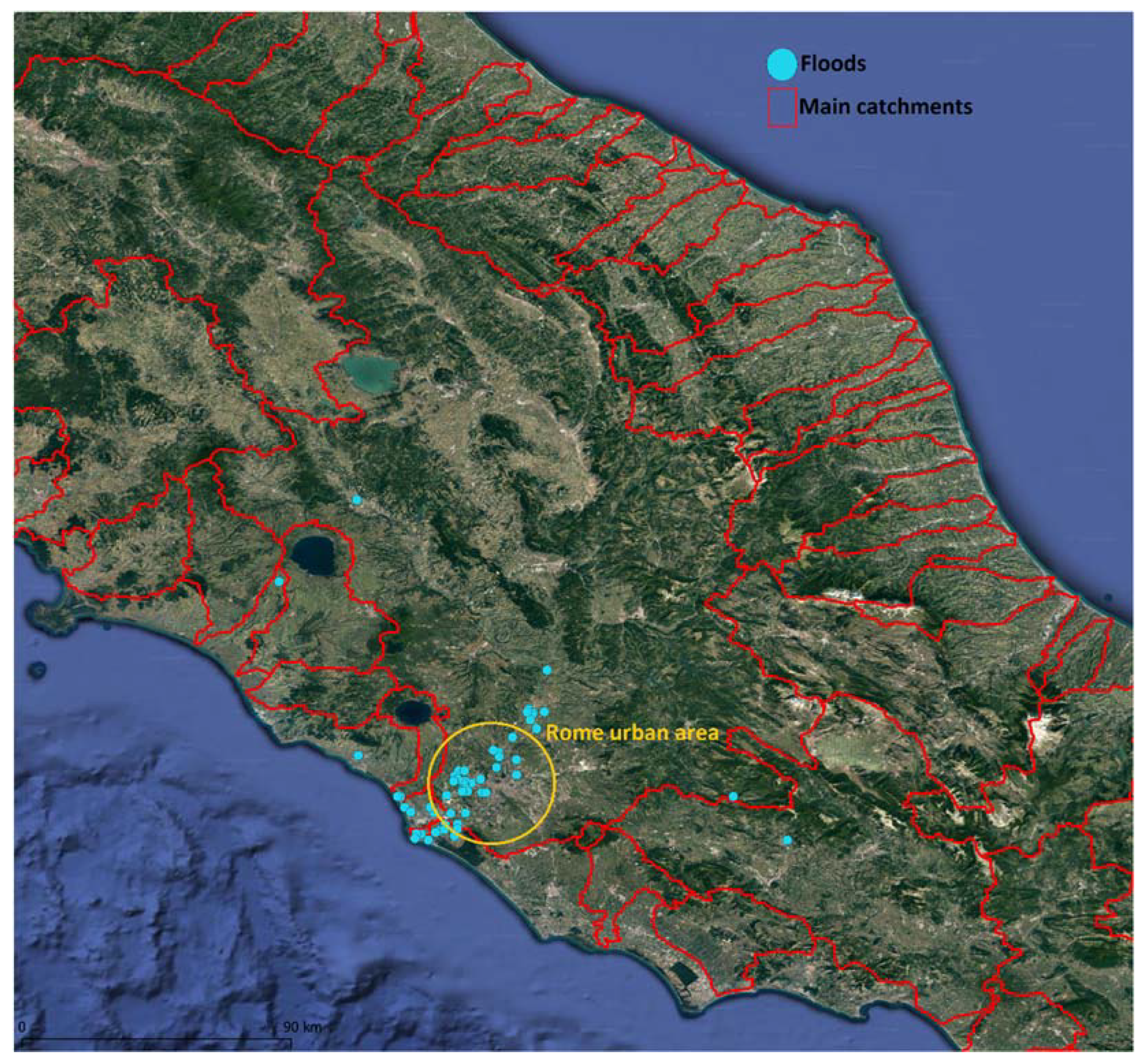
Qualitative data consisted of all the available information on flooding, inundations, or slope instabilities caused by intense runoff. Most of these data were collected by the Umbria and Lazio Regions Functional Centers and are documented in their official severe weather event reports. A detailed description of rainfall-triggered landslides affecting the Rome metropolitan area were reported by Alessi et al. [26]. Each phenomenon was geo-referred and time-referred, indicating the day of occurrence (Figure 1 and Figure 2). Qualitative data, integrated with measurements, were used to validate the spatial distribution of hydrological and hydro-geological stress simulated in the basin, since they included relevant information for those areas where instruments were not installed.
Quantitative data included a water level hourly time series provided by the network of hydrometers installed across the basin. Hourly hydrometric height data were downloaded from the Dewetra platform [27] with hourly temporal resolution for the dates of the event. A list of all available hydrometric measurements for this case study is provided in the Supplementary Material, Table S1. That table also reports hydrological criticality thresholds for those stations where thresholds have been defined by regional functional centres according to guidelines provided by the Italian Civil Protection Department (2008). To better organize our analysis, the Tiber basin was divided into three geographical areas: (i) the upper course, corresponding to the area upstream to the Corbara Dam; (ii) the middle course, including the Velino, Nera, and Paglia sub-basins; and (iii) the lower course, which ranges from the confluence with the Aniene tributary to the outlet.

4. Hydrological Simulation

Hydrological and hydro-geological stress indices for the selected case study (BDD, CAI, and LAI) were calculated starting with a hydrological simulation of the Tiber basin using the Cetemps Hydrological Model (CHyM) [28]. The model was developed and is being continuously updated at the CETEMPS, Center of Excellence of the University of L’Aquila, Italy. The model has been used and calibrated in Italy for many purposes, including flood alert mapping [29,30,31,32], climatological studies [33,34], and water quality [35,36]. Since the CETEMPS is appointed as civil protection competence center, at both national and regional (Abruzzo) level, the model outputs and the CHyM alert mapping products presented in this study are officially released twice a day, as part of the EWS to hydro-geological risk. All relevant physical quantities are defined on an equally spaced grid with a horizontal resolution in the order of hundreds of meters, which is usually chosen according to the morphological characteristics of the domain and available computational resources. CHyM can be used to simulate the hydrological cycle of any geographical domain with any spatial resolution of up to 90 m, which is the resolution of the digital terrain model implemented in this study. An interpolation technique based on cellular automata theory was used to correct terrain elevation singularities, in order to rebuild the drainage network. The same technique was also used to spatialize meteorological input (rainfall and temperature) that could either be organized on a regular grid or as sparse point-data [37]. The CHyM model is currently used for operational flood prediction in Italy, Croatia, and Albania through the daily release of hydrological stress indices maps (https://cetemps.aquila.infn.it/chymop/, accessed on 1 July 2022). Since a complete description of the physics of the model would be redundant and beyond the aim of this current paper, the calculation schemes adopted to simulate hydrological processes are summarized in Table 1. A more complete description can be found in Verdecchia et al. [28] or Coppola et al. [34] Nevertheless, a more detailed characterization of the CHyM model calculation schemes is also provided in the Supplementary Materials.
For this event, the model simulation was initiated at 00 UTC on 25 January 2014 and concluded at 00 UTC on 6 February 2014. The severe weather event occurred from 31 January to 4 February 2014; therefore, six days of spin-up time were chosen to initialize the hydrology of the target catchment, according to information provided by Bersani and Bencivenga [38].
The spatial horizontal resolution of the entire domain was set to 666 m (0.006 deg), with an hourly temporal resolution. Meteorological inputs of hourly rainfall and air temperature were provided by the Civil Protection gauge network and downloaded from the Dewetra platform, including data from 528 working thermo-pluviometric stations in the area.

5. Stress Indices

The BDD (Best Discharge-based Drainage Index) and CAI (Chym Alarm Index) calculation methods are detailed in Lombardi et al. [29], while experiments with the LAI (Landslide Activation Index) application was first reported in Tomassetti et al. [39]. In summary, the BDD index is calculated for each hourly time-step and each grid-point i,j of the geographical domain according to the following formula:
B D D i , j = Q i , j R i , j 2
where Qi,j is the discharge value predicted in the grid-point by the CHyM model and Ri,j is the grid-point hydraulic radius, which is proportional to the upstream drained area.
The CAI index is linked to the surface runoff rate, rather than the simulated river discharge. As with the BDD index, the CAI refers to each time step and each grid-point of the drainage network, but computation requires information from the entire upstream area, i.e., total precipitation accumulated during the mean concentration time. Therefore, before carrying out the CAI calculation, average runoff time from any point of the upstream area to the ith–jth grid point must be calculated. Then, total precipitation (Pr) through the grid point during mean concentration time can be computed. The CAI formula for each time step and each grid point i,j is as follows:
C A I i , j = U P   t t + t P r d t d s U P   d s
where the integral is calculated over space s and time t across the upstream area (UP) in a time interval corresponding to the concentration time Δt.
Lombardi et al. [29] highlighted the different approaches of these two hydrological indices. The BDD index is physically based and depends on calculated river discharge resulting from the balance of different hydrological processes, while the CAI index is an empirical index that strictly depends on precipitation.
The dependence of the CAI index on precipitation suggests its applicability over slopes, where rapid surface runoff may lead to solid transportation and evolve into landslide events triggered by heavy rainfall. Consequently, the LAI index was developed to extend the concept of the CAI index to slope stability, in order to gain information on hydro-geological stress due to intense runoff rates occurring within a certain lag time. The LAI index is an estimation of hydrological stresses limited to the effects of excessive runoff. It is not meant to predict wet mass movement itself, which is strongly dependent on the geological and lithological features of the land, as well as slope inclination and exposition, which are not included in the index calculation. In addition, the index takes into account the quantity of precipitation drained from the terrain slopes related to mean concentration time, so that it may be interpreted as an estimation of the intensity of the meteorological process likely to trigger a wet mass movement event.
BDD, CAI, and LAI indices threshold values (Table 2) were calibrated and experimentally refined during more than 10 years of operational application for flood prediction, as a consequence of a specific agreement with the Civil Protection Central Functional Center (project IDRA2), the Abruzzo and Marche Region Functional Centers (project AdriaRadNet). The daily stress-based forecast release is available at: http://cetemps.aquila.infn.it/chymop (accessed on 1 July 2022).

6. Statistical Analysis

Spatial and temporal validation of BDD and CAI indices were carried out by means of dichotomous analysis using contingency tables-based scores that compared indices threshold exceedances with hydrometric level exceedances at each station point. For each hourly value of BDD and CAI indices, the exceedance/non-exceedance of the index value, with respect to its moderate threshold, was detected. The exceedance/non-exceedance event was then compared with the hourly hydrometric level value exceeding/not exceeding the moderate criticality threshold, as defined by the civil protection authorities according to the current regulations. The analysis was carried out for all 31 hydrometers with officially defined criticality thresholds (25 in the Tiber basin, 2 in the Liri-Garigliano, and 1 in the northern Lazio basins). The score was calculated on the moderate threshold only, as this represented the minimum criticality level to begin the operative phases that require direct local authority involvement. The moderate hydrometric level (orange) threshold was compared with the moderate stress threshold defined for the two indices. Each hourly water level event of exceedance/non-exceedance at each station point was compared with the corresponding value of the BDD and CAI indices, calculated at the grid-point co-located with the gauge’s coordinates. The temporal comparison was carried out over a period of ±1 h. Prediction accuracy (A), probability of detection (POD), and false alarm rate (FAR) were then calculated for both the BDD and CAI indices.
A contingency table was also built to test the LAI index response in detecting landslide stress, given that no continuous hydrological variable time series can be directly associated with landslide activation. Therefore, rainfall-induced mass movement was considered a Boolean event (occurrence/non-occurrence). For this reason, all three LAI threshold (ordinary, moderate, and high) exceedances were compared to the occurrence/non-occurrence of mass movements and only the POD was calculated, since a false positive indicated by the LAI index could not be verified. For example, the LAI index may identify an activation in which no wet mass movement is possible, due to the absence of a suitable substratum. The LAI index stress map should overlay a landslide susceptibility map, in order to refine the index information for those areas where rainfall-induced mass movement can potentially occur. However, this information was not available for all of the investigated areas, although some local attempts at gathering such data have been made in central Italy [40,41,42,43].
In addition, a continuous time series analysis was applied for BDD and CAI indices validation in order to relate the indices temporal profiles with the river stage profile. This analysis considered water level and index profile as signals. The temporal coherence between CAI, BDD, and normalized river stage values was investigated using statistical scores typically used in signal analysis. A complete overview of the evaluated variables can be found in Lombardi et al. [29]; however, a summary of the proposed indices and their significance is shown in Table 3.

7. Case Study Description

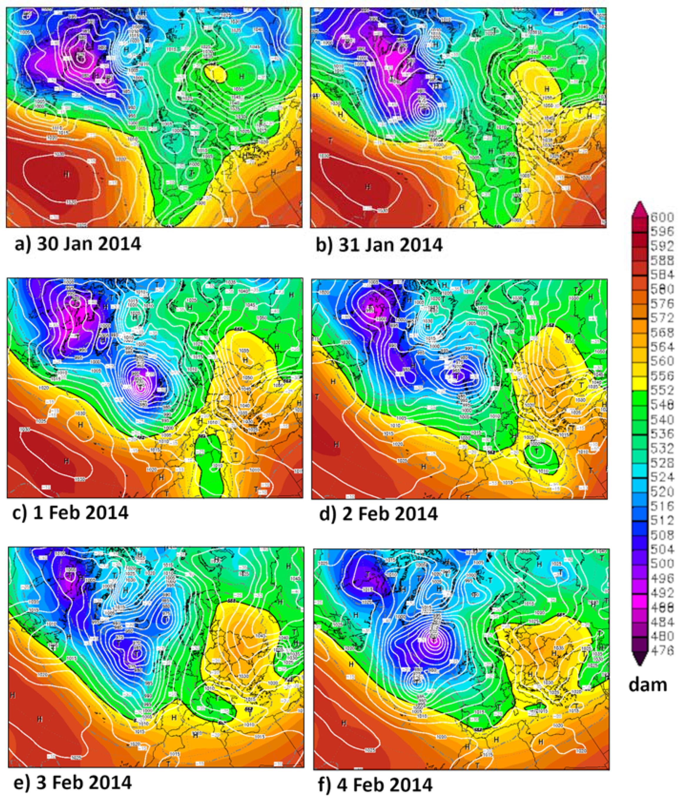
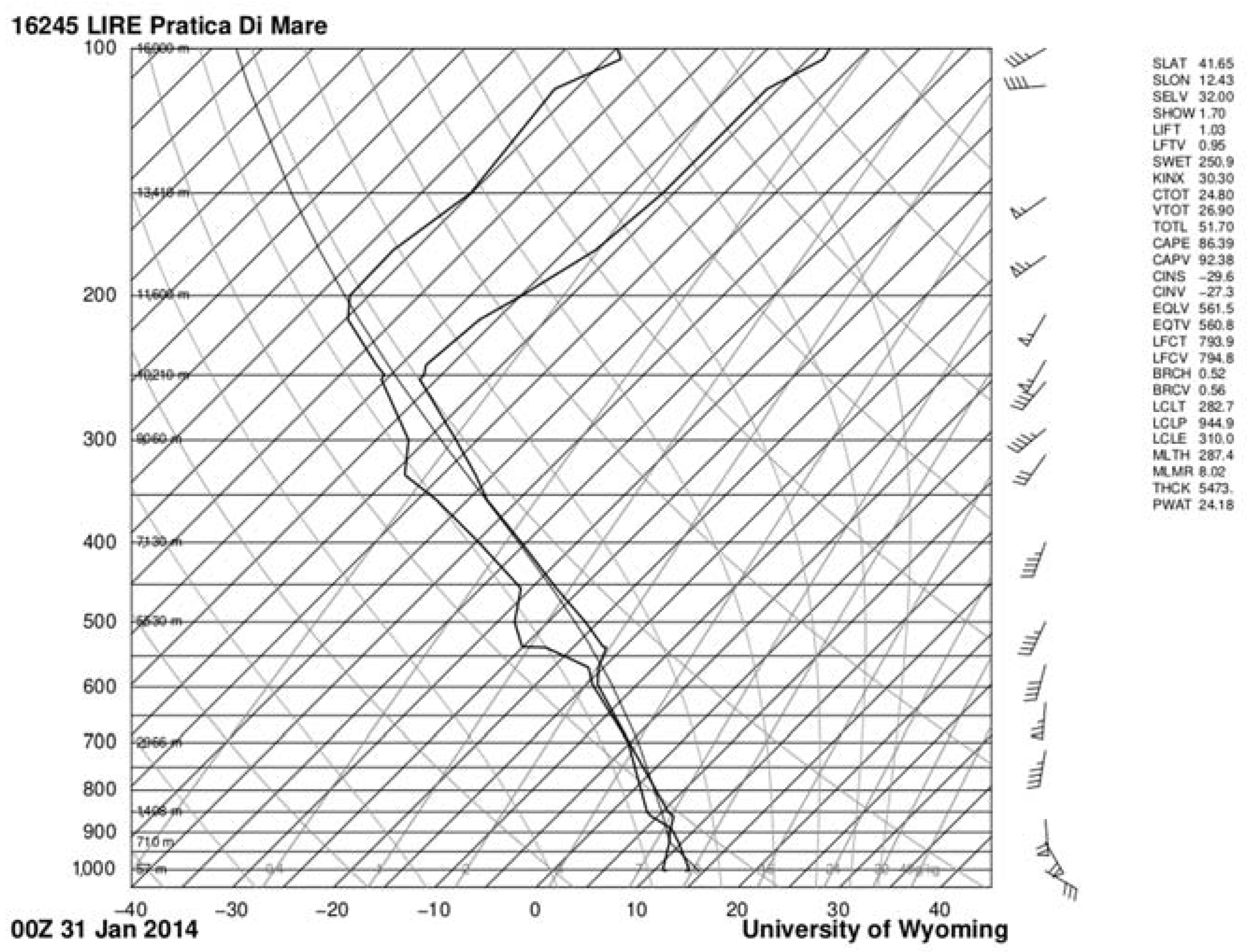
The period from 30 January to 4 February 2014 was characterized by intense severe weather, which resulted in abundant rainfall over a wide area of central Italy. The peak of extreme weather, corresponding to maximum precipitation rates, was recorded on 31 January, when a flood event occurred in the Lazio region, with particular intensity in the province of Rome. As shown in the weather report issued by the Lazio Region Functional Center [47], the 6-day event affected many river basins in the Umbria, Lazio, and Campania regions. In particular, northern coastal Lazio basins (NL-B), all of the Tiber basin (TR-B), and the northern section of the Liri-Garigliano basin (LG-B) were affected. The flood in TR-B propagated from north to south and the discharge maxima occurred between 31 January and 1 February, starting from the upper TR-B and Umbria Region tributaries. In the main Aniene River, the principal tributary of the Tiber, floodings were recorded on 1 February, while the LG-B discharge maxima were recorded between 1 and 2 February 2014. The perturbed system was activated on 30 January by a descending well-structured weather trough in the central-western Mediterranean, which moved a moist air mass of polar-maritime origin towards the Algerian hinterland (Figure 3a). As a consequence, the Tyrrhenian side of the Italian peninsula was hit by a warm and moist southern airmass flow. At the same time, a cyclogenesis originating in the Ligurian Sea, and the reinforcement of the zonal current in central Europe caused the formation of a cutoff over North Africa the following day (Figure 3b). The trough, associated with a deep baric minimum centred on the north Atlantic, hovered over the Tyrrhenian Sea in the following days (Figure 3c–f), triggering moderate precipitation which persisted in southern Lazio until 5 February. At night, between 30 and 31 January, an extensive V-shaped storm system caused by the Scirocco developed in the middle of the Tyrrhenian Sea along a line of confluence at ground level between moist and warm southern currents and cooler western currents. The perturbed front was slow in its evolution toward the Levant, due to a blocking synoptic configuration over Eastern Europe, affected by a wide ridge of ~1055 hPa of maxima baric pressure at ground level. This caused persistent precipitation in the medium-lower Tiber basin for most of the day of 31 January. A more qualitative analysis of the thermodynamic conditions in the Lazio region is provided by the 00 UTC atmospheric sounding from Pratica Di Mare, near the city of Rome (41.65° N, 12.43° E); from the skew-T diagram reported in Figure 4, a substantially saturated column of air can be observed from the first atmospheric layers, with the lifting condensation level (LCL) positioned at 944.9 hPa, a favourable condition for the rapid development of clouds. Moreover, the presence of significant shear determined the persistence of intense convective structures.
Rainfall maxima occurred along the terminal path of the Tiber River, where values of ~200 mm/48 h were recorded at the Octavia (201.8 mm/48 h) and Riano (202.0 mm/48 h) rain gauges, corresponding to a 200-year return period (Figure 5).
Damage was reported in 80 Lazio municipalities, including destruction of infrastructure due to wet mass movement (impassable roads, unsafe buildings, damages to sewer systems, interruption of electrical infrastructure) and flooding. Local authorities decided to evacuate more than 500 people. The Corbara, Alviano, Ponte Felice, Nazzano, and Castel Giubileo dams were forced to conduct flood lamination draining operations. The report of the Lazio Functional Center only provides information about operations at the Corbara and Alviano reservoirs. In particular, the Corbara Dam, located in the upper Tiber catchment, discharged up to 700 m3/s downstream to the middle course of the river between 31 January and 2 February. The Alviano reservoir released almost 1000 m3/s in the same period.
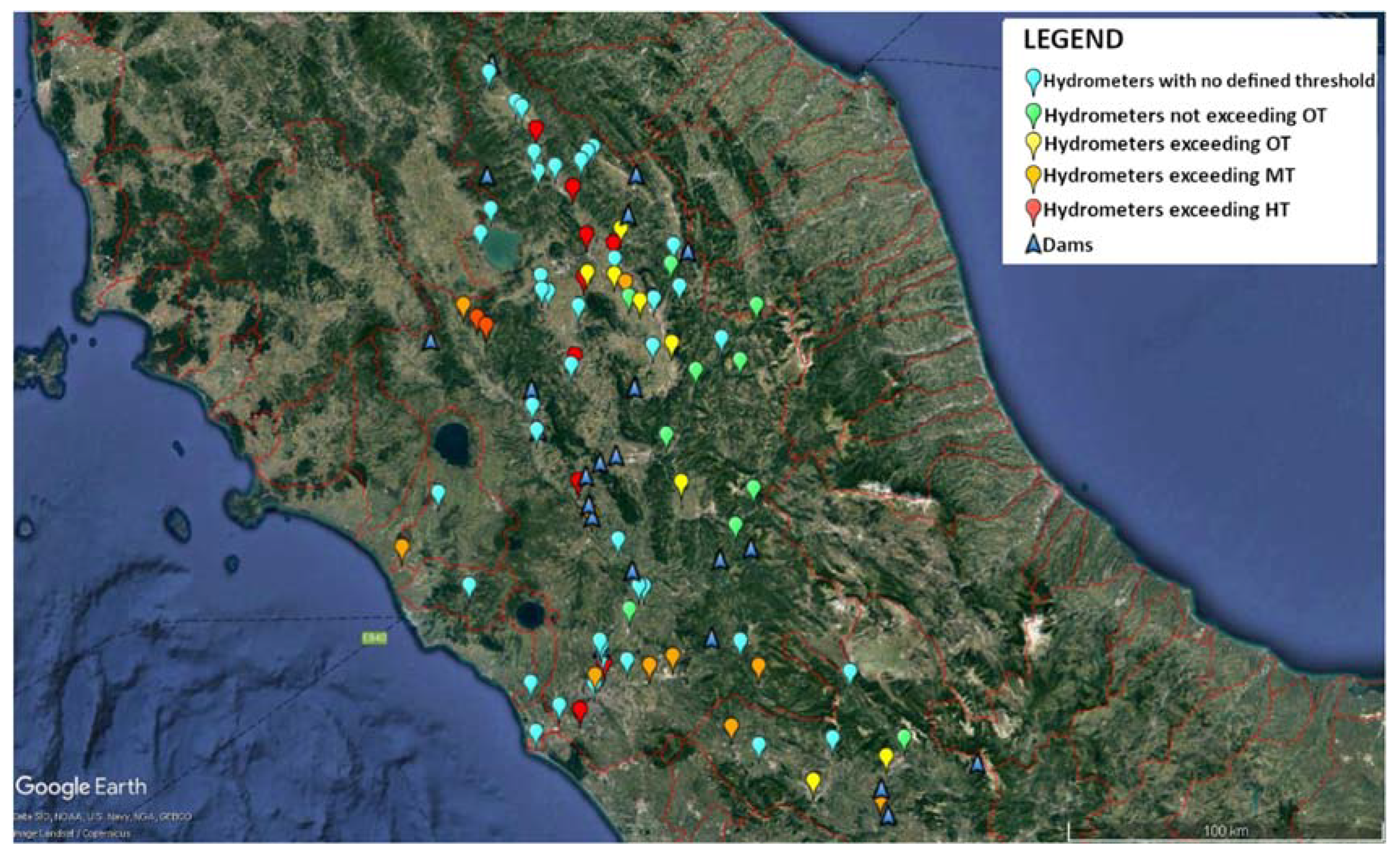
Critical water level thresholds have been defined by civil protection authorities for 34 hydrometric stations across the three basins. During the event, 8 stations recorded hydrometric levels exceeding the ordinary threshold (OT), 11 exceeded the moderate threshold (MT), and 10 exceeded the high threshold (HT). The water level time series for the remaining sensors remained below the OT (Figure 6).

8. Results and Discussion

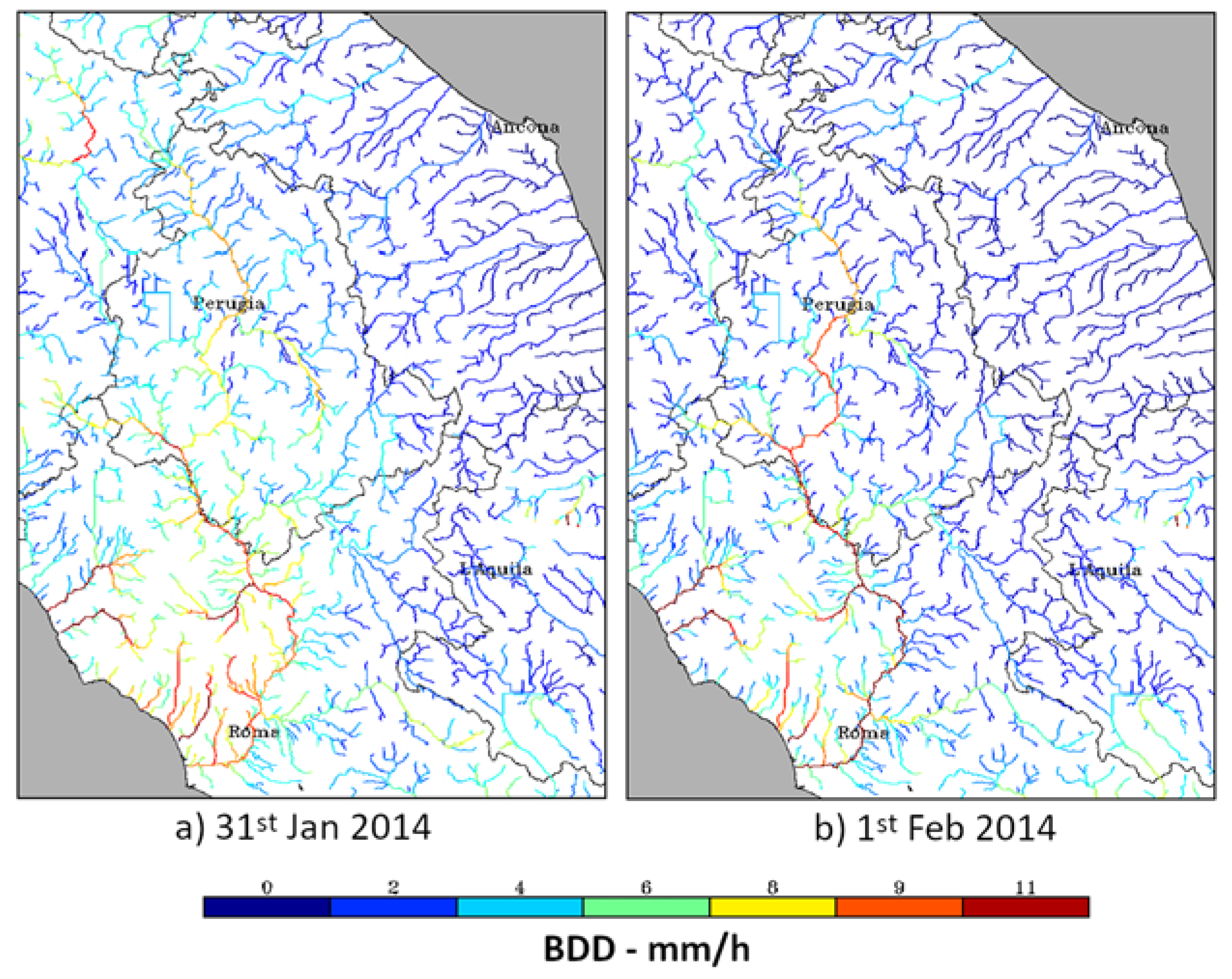
Figure 7 and Figure 8 show daily BDD and CAI maps for 31 January and 1 February 2014, the main days of the weather event. Both images were obtained by representing the maximum daily index value found at each grid-point of the drainage network; therefore, they are not synchronic maps referring to a specific hour of the day. This representation allows a general overview of the possible location of the most stressed river segments within 24 h, even when the weather event was evolving rapidly, causing flood occurrences at different time periods throughout the day. The event’s hour-by-hour temporal evolution can be investigated by observing a sequence of 24-hourly maps (not shown). The BDD index highlights the middle and lower course of the main branch of the Tiber River after the confluence of the Topino and Chiascio Rivers, where most of the inundation, as well as MT and HT exceedances, were reported. The upper part of the Tiber branch was characterized by low BDD values, although five sensors along the river path exceeded HT. In this area, the simulated hydrological stress result proved to be an underestimation. Ordinary to moderate stress was simulated in the final segment of the Aniene River before it joins the Tiber, and hydrologic criticality was slightly underestimated. Nevertheless, the highest BDD values were found in the lower Tiber, where the event was particularly severe. The hydrological stress simulated in NL-B was indicated by MT exceedance on the Marta River (station “Marta a Tarquinia”), which is the only river section in the area with defined criticality thresholds. In this case, the BDD index coherently indicated a moderate stress condition over the Marta branch. As for the LG-B upper basin, the index simulated ordinary hydrological stress, which was a slight underestimation.
The CAI hydrological stress spatial distribution was significantly different to that of the BDD. The main river branches, such as the Tiber and the Aniene, did not reach moderate or high stress conditions. However, almost the entire secondary drainage network, including the smallest tributaries, was observed to reach a significant hydrological stress status (above CAI moderate and high thresholds). Moreover, CAI identified moderate stress conditions in the north-eastern part of the Tiber basin (north of Perugia), where the BDD signal was weak. All Tiber tributaries (except for the Aniene) were highlighted and almost all of the north-western part of the watershed was under high stress. Since the secondary network is poorly gauged, it was not possible to establish if the CAI signal was overestimated in this area. In NL-B, the CAI index accentuated hydrological stress over small tributaries in the Marta catchment, as well as the Arrone River. The Marta main branch (with a drainage area of ~1000 km2) is the only river which had high threshold result in both indices.
A more objective assessment of the spatial coherence between the indices and the displacement of critical hydrological events is provided by contingency table scores, as reported in Table 4. The accuracy values for the BDD index were generally higher than 0.9, with the exception of the lower course of the Tiber, where A decreased to 0.74. FAR values were negligible in most cases, even if a slight stress overestimation resulted from the BDD signal in the upper course of the Tiber (FAR = 0.22). This last result was strongly influenced by the Ponte Osteria station, where MT was exceeded for only one hour, while the BDD index indicated a moderate stress threshold for ~15 h. The highest POD for BDD was obtained on the upper Tiber. The score then decreased, as the number of missed exceedances increased downstream due to lamination effects. The best BDD result was obtained at the “Marta a Tarquinia” river station. In the LG-B stations, index values remained below the MS, so that exceedance of the MT was not detected.
For the TR-B, the decreasing quality of statistical scores from the upper to lower part of the Tiber basin was noticeable. The effect was particularly evident in the POD values, which ranged from a highest value of 0.83, progressively decreasing to less than 0.5 in the lower course of the river. The decreasing quality of the score was affected by the high quantity of missing moderate threshold exceedances in the BDD index, which were mainly concentrated in both the lower course of the Tiber and in its primary tributary, the Aniene. CAI index scores were similar in accuracy, but POD values were much lower in TR-B. This effect was mainly due to the absence of hydrometric stations along the smallest tributaries, where the CAI index highlighted the maximum stress. As evidenced in Figure 6, the CAI index did not identify hydrological stress over the widest catchments, where most of the sensors are installed. Similar results were obtained by Alfieri & Thielen [48]. The hydrological stress index (EPIC) developed by the authors resulted in a POD of ~90% over small catchments (<2000 m2) for FFs events, while FLs events were less detectable by the index. Nevertheless, FAR was 56%.
An assessment of correct timing information provided by the BDD and CAI indices is shown in Table 5. This table also shows a breakdown of timing scores for the Tiber basin subunits. In this case, the effect of a time shift of peak discharge due to lamination activities significantly affected the results, especially in the middle course of the Tiber which starts just after the Corbara Dam, the largest water reservoir in the TR-B.
Worsening space-time location of both indices from north to south was due to the increasing impact of anthropic regulation on the many reservoirs built along the main branch of the Tiber and its main tributaries. However, timing in the lower TR-B was more accurate than upstream. This result was affected by the statistical scores of the Aniene catchment, where the timing of the simulated indices and observed data showed higher synchronicity. In the main branch of the Tiber, the lamination of the flood wave which propagated from higher to lower latitudes progressively altered the natural flow, resulting in a discrepancy between modelled and real overflow dynamics that became amplified in a southward direction.
The DDTW (Table 6) and the CTD take the increasing/decreasing rate of the two compared signals into account, while also considering their time-shift. CTD values were generally ~1 h, while DDTW values were close to the optimal value (a zero-value corresponds to a perfect overlap). This last outcome suggests that both indices are capable of describing the evolution of the hydrometric level and are representative of a hydrological hazard resulting from flood wave propagation. Our comparison of CAI and BDD indices shows similar results to Corral et al. [49], where two hydrological stress indices based on precipitation thresholds and discharge computed by a hydrological model were applied for flood forecasting. In their study, authors found that the ERICHA index, based on precipitation thresholds, is able to detect short-duration phenomena, such as flash flood events. To forecast a more complex and longer flood event over wider basins, the computation of the discharge was needed to obtain better results. Even if our conclusions are similar to those of other authors who implemented indices for different kind of floods detection, the indices thresholds determination is remarkably different. Actually, both Corral et al. [49] and Alfieri & Thielen [8] determined indices threshold basing on local climatology, therefore, indices thresholds are different for different basins. In our case, the BDD and CAI computation takes implicitly into account the basins dimension, and therefore our alert thresholds (see Table 2) are the same in any point of the drainage network. As a consequence, the climatological indices calibration is unnecessary in our case.
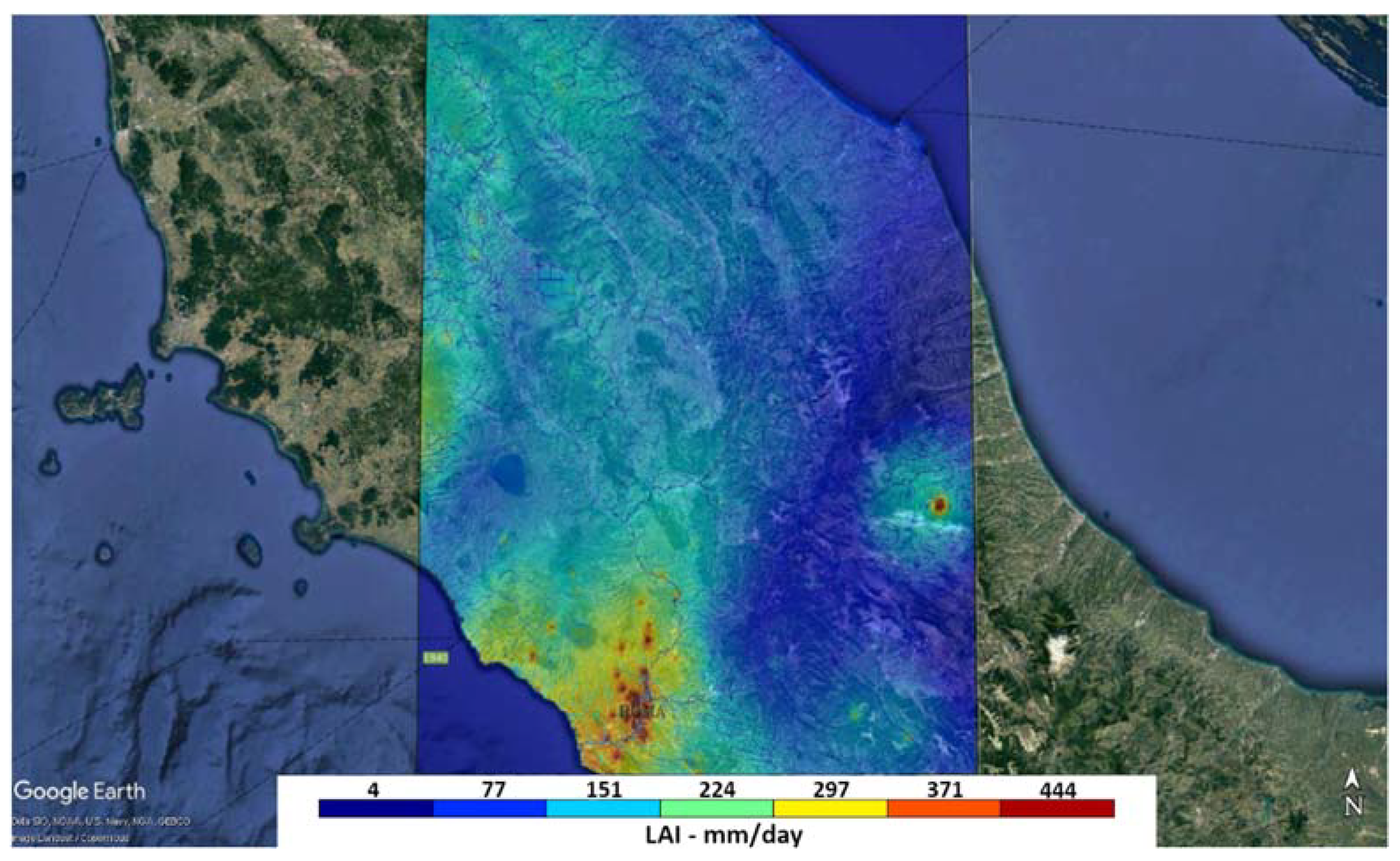
In addition, according to the official event report and local news reports, 111 landslides were reported for this weather event. The LAI daily map for 31 January 2014, covering the entire area, is shown in Figure 9. Of the reported landslides, 77% were triggered by heavy rain, and thus associated with LAI ordinary stress threshold exceedance, while 51% exceeded the moderate threshold. Higher peaks exceeding the high LAI threshold account for 37% of wet mass movements, which were mainly concentrated in the Rome metropolitan area. A moderate-to-ordinary stress, precursor of possible landslide activation, was also shown in the LG-B upper basin, along the southern boundary of the spatial domain. In the same area, one third of mass movements were recorded. Finally, only one landslide event, which occurred north of Bracciano Lake, was completely missed by the index.

9. Conclusions

The validation of a unique model-based application for identifying different rainfall-related hydrogeological stress conditions was presented in this work. The application is based on the CHyM hydrological distributed model and was thought to be applied in the context of civil protection early warning, providing an effective tool for the prediction of different phenomena.
Three hydrological stress indices were evaluated during a severe weather event, which caused several floods and landslides in central Italy. The flood-related indices, BDD and CAI, showed an accuracy >90% in identifying moderate stressed river segments, as well as very low values of false alarms, close to zero in most cases. However, the results differed with the catchment size and the heavy anthropic exploitation of the Tiber basin for hydropower production significantly affected timing results.
The LAI hydrogeological index was tested on 111 landslide events triggered by rainfall. The LAI lowest threshold allowed the identification of 77% of the recorded events over the entire domain of central Italy. In addition, the high LAI threshold identified the occurrence of landslides in metropolitan Rome. In general, main outcomes can be summarized as follows:
  • The BDD index is responsive to fluvial floods, generated over basins with extension greater than ~1000 km2;
  • The CAI index is more responsive to rapid flood phenomena, typical of smallest basins (flash floods);
  • The BDD and CAI timing with respect to fluvial and pluvial floods are accurate upstream, while the shift between the observed and simulated discharge peak increases downstream;
  • The LAI index is more responsive in the prediction in an urban context.
Stress conditions are identified through the use of indices to detect areas affected by FLs, FFs, and RLs. Moreover, the responsiveness of indices may represent a useful instrument for discriminating the evolution of FLs and FFs over complex basins, since all these phenomena are driven by the different interactions of rainfall with the landscape.

Supplementary Materials

The following supporting information can be downloaded at: https://www.mdpi.com/article/10.3390/hydrology9080139/s1.

Author Contributions

V.C., D.G., A.L. and B.T.: manuscript writing; V.C., A.L. and B.T.: conceptualization and design; V.C., A.L., B.T., D.G., E.R. and P.T.: formal analysis; R.L.: technical assistance; V.C., A.L., B.T., E.R., P.T., R.L. and M.V.: draft revision. V.C., A.L. and B.T. gave equal contribution to the work. All authors have read and agreed to the published version of the manuscript.

Funding

This research received no external funding.

Data Availability Statement

The data presented in this study are available on request from the corresponding author. The CHyM simulation outputs are in own native format and needs to be converted in other public format on request. The hydro-meteorological data are from third parties and needs to be requested to the hydrographic services of Lazio Region (https://protezionecivile.regione.lazio.it/gestione-emergenze/centro-funzionale/servizio-idrografico, accessed on 29 June 2022), Umbra Region (https://www.regione.umbria.it/ambiente/servizio-idrografico, accessed on 29 June 2022), Marche Region (https://www.regione.marche.it/Regione-Utile/Protezione-Civile/Progetti-e-Pubblicazioni/Annali-Idrologici, accessed on 29 June 2022) and Abruzzo Region (https://www.regione.abruzzo.it/content/idrografico-mareografico, accessed on 29 June 2022).

Conflicts of Interest

The authors declare no conflict of interest.

References

  1. Llasat, M.C.; Llasat-Botija, M.; Prat, M.A.; Porcú, F.; Price, C.; Mugnai, A.; Lagouvardos, K.; Kotroni, V.; Katsanos, D.; Michaelides, S.; et al. High-impact floods and flash floods in Mediterranean countries: The FLASH preliminary database. Adv. Geosci. 2010, 23, 47–55. [Google Scholar] [CrossRef] [Green Version]
  2. Paliaga, G.; Faccini, F.; Luino, F.; Roccati, A.; Turconi, L. A clustering classification of catchment anthropogenic modification and relationships with floods. Sci. Tot. Env. 2020, 740, 139915. [Google Scholar] [CrossRef]
  3. Tarasova, L.; Merz, R.A.; Kiss, A.; Basso, S.; Blöschl, G.; Merz, B.; Viglione, A.; Plötner, S.; Guse, B.; Schumann, A.; et al. Causative classification of river flood events. WIREs Water 2019, 6, e1353. [Google Scholar] [CrossRef] [Green Version]
  4. Hammond, M.J.; Chen, A.S.; Djordjević, S.; Butler, D.; Mark, O. Urban flood impact assessment: A state-of-the-art review. Urban Water J. 2013, 12, 14–29. [Google Scholar] [CrossRef] [Green Version]
  5. Seong, C.; Heejun, C. Recent research approaches to urban flood vulnerability, 2006–2016. Nat. Hazards 2022, 88, 1–17. [Google Scholar]
  6. Zhong, Q.; Wang, L.; Chen, S.; Shan, Z.; Shan, Q.; Ren, Q.; Mei, S.; Jiang, J.; Hu, L.; Liu, J. Breaches of embankment and landslide dams - State of the art review. Earth-Sci. Rev. 2021, 2016, 103597. [Google Scholar] [CrossRef]
  7. Moramarco, T.; Barbetta, S.; Pandolfo, C.; Tarpanelli, A.; Berni, N.; Morbidelli, R. Spillway collapse of the Montedoglio Dam on the Tiber River, Central Italy: Data collection and event analysis. J. Hydrol. Eng. 2014, 19, 1264–1270. [Google Scholar] [CrossRef]
  8. Manfreda, S.; Miglino, D.; Albertini, C. Impact of detention dams on the probability distribution of floods. Hydrol. Earth Syst. Sci. 2021, 25, 4231–4242. [Google Scholar] [CrossRef]
  9. Ridolfi, E.; Di Francesco, S.; Pandolfo, C.; Berni, N.; Biscarini, C.; Manciola, P. Coping with Extreme Events: Effect of Different Reservoir Operation Strategies on Flood Inundation Maps. Water 2019, 11, 982. [Google Scholar] [CrossRef] [Green Version]
  10. ISPRA. Dissesto Idrogeologico in Italia: Pericolosità e Indicatori di Rischio (Hydrogeological Instability in Italy: Danger and Risk Indicators); Report No. 287; ISPRA: Roma, Italy, 2018; ISBN 978-88-448-0901-0. Available online: https://www.isprambiente.gov.it/files2018/pubblicazioni/rapporti/rapporto-dissesto- (accessed on 29 June 2022).
  11. Marchesini, I.; Ardizzone, F.; Alvioli, M.; Rossi, M.; Guzzetti, F. Non-susceptible landslide areas in Italy and in the Mediterranean region. Nat. Hazards Earth Syst. Sci. 2014, 12, 2215–2231. [Google Scholar] [CrossRef] [Green Version]
  12. Kobiyama, M.; Goerl, R.F. Quantitative method to distinguish flood and flash flood as disasters. Hydrol. Res. Lett. 2007, 1, 11–14. [Google Scholar] [CrossRef] [Green Version]
  13. Wohl, E. The complexity of the real world in the context of the field tradition in geomorphology. Geomorphology 2013, 200, 50–58. [Google Scholar] [CrossRef]
  14. Smith, P.J.; Brown, S.; Dugar, S. Community Based Early Warning Systems for flood risk mitigationin Nepal. Nat. Hazards Earth Syst. Sci. 2017, 17, 423–437. [Google Scholar] [CrossRef] [Green Version]
  15. World Meteorological Organization–WMO. Management of Flash Floods, Integrated Management Tools Series no.16, Issue 16, May 2012. 2014. Available online: https://library.wmo.int/doc_num.php?explnum_id=7337 (accessed on 20 December 2021).
  16. Georgakakos, K.P. On the design of natural, real-time warning systems with capability for site-specific, flashflood forecasts. Bull. Am. Meteorol. Soc. 1986, 67, 1233–1239. [Google Scholar] [CrossRef]
  17. Turkington, T.; Breinl, K.; Ettema, J.; Alkema, D.; Jetten, V. A new flood type classification method for use in climate change impact studies. Weather. Clim. Extrem. 2016, 14, 1–16. [Google Scholar] [CrossRef] [Green Version]
  18. Alfieri, L.; Burek, P.; Feyen, L.; Forzieri, G. Global warming increases the frequency of river floods in Europe. Hydrol. Earth Syst. Sci. 2015, 19, 2247–2260. [Google Scholar] [CrossRef] [Green Version]
  19. Endo, T. Probable Distribution of the Amount of Rainfall Causing Landslides; Annual Report, Hokkaido Branch, 1970; Govern Forest Experiment Station: Sapporo, Japan, 1970; pp. 123–136. [Google Scholar]
  20. Oakley, N.S.; Lancaster, J.T.; Hatchett, B.J.; Stock, J.; Ralph, F.M.; Roj, S.; Lukashov, S. A 22-Year Climatology of Cool Season Hourly Precipitation Thresholds Conducive to Shallow Landslides in California. Earth Interact. 2018, 22, 1–35. [Google Scholar] [CrossRef]
  21. Guzzetti, F.; Peruccacci, S.; Rossi, M.; Stark, C.P. Rainfall thresholds for the initiation of landslides in central and southern Europe. Meteorol. Atmos. Phys. 2007, 98, 239–267. [Google Scholar] [CrossRef]
  22. Segoni, S.; Piciullo, L.; Gariano, S.L. Preface: Landslide early warning systems: Monitoring systems, rainfall thresholds, warning models, performance evaluation and risk perception. Nat. Hazards Earth Syst. Sci. 2018, 18, 3179–3186. [Google Scholar] [CrossRef]
  23. Guzzetti, F.; Gariano, S.L.; Peruccacci, S.; Brunetti, M.T.; Marchesini, I.; Rossi, M.; Melillo, M. Geographical landslide early warning systems. Earth-Sci. Rev. 2020, 200, 102973. [Google Scholar] [CrossRef]
  24. Arredi, F. Brevi richiami alle caratteristiche del Tevere (Short notes on the Tiber characteristics). In Idrotecnica 1; Gentile-Feb.: Roma, Italy, 1974. [Google Scholar]
  25. Raparelli, E.; Tuccella, P.; Colaiuda, V.; Marzano, F.S. Snow cover prediction in the Italian Central Apennines using weather forecast and snowpack numerical model. Cryosphere Discuss. 2021, 285. [Google Scholar]
  26. Alessi, D.; Bozzano, F.; Di Lisa, A.; Esposito, C.; Fantini, A.; Loffredo, A.; Martino, S.; Mele, F.; Moretto, S.; Noviello, A.; et al. Geological risk in large cities: The landslides triggered in the city of Rome (Italy) by the rainfall of 31 January–2 February 2014. Ital. J. Eng. Geol. Environ. 2014, 1, 15–34. [Google Scholar]
  27. Italian Civil Protection Department; CIMA Research Foundation. The Dewetra Platform: A Multi-perspective Architecture for Risk Management during Emergencies. In Information Systems for Crisis Response and Management in Mediterranean Countries; Hanachi, C., Bénaben, F., Charoy, F., Eds.; ISCRAM-med 2014, Lecture Notes in Business Information Processing; Springer: Cham, Switzerland, 2014; pp. 165–177. [Google Scholar]
  28. Verdecchia, M.; Coppola, E.; Tomassetti, B.; Visconti, G. Cetemps Hydrological Model (CHyM), a Distributed Grid-Based Model Assimilating Different Rainfall Data Sources. In Hydrological Modelling and the Water Cycle; Sorooshian, S., Hsu, K.L., Coppola, E., Tomassetti, B., Verdecchia, M., Visconti, G., Eds.; Water Sciences Technol. Library; Springer: Berlin/Heidelberg, Germany, 2008; Volume 63, pp. 165–201. [Google Scholar]
  29. Lombardi, A.; Colaiuda, V.; Verdecchia, M.; Tomassetti, B. User-oriented hydrological indices for early warning systems with validation using post-event surveys: Flood case studies in the Central Apennine District. Hydrol. Earth Syst. Sci. 2021, 25, 1969–1992. [Google Scholar] [CrossRef]
  30. Ferretti, R.; Lombardi, A.; Tomassetti, B.; Sangelantoni, L.; Colaiuda, V.; Mazzarella, V.; Maiello, I.; Verdecchia, M.; Redaelli, G. A meteorological–hydrological regional ensemble forecast for an early-warning system over small Apennine catchments in Central Italy. Hydrol. Earth Syst. Sci. 2020, 24, 3135–3156. [Google Scholar] [CrossRef]
  31. Colaiuda, V.; Lombardi, A.; Verdecchia, M.; Mazzarella, V.; Ricchi, A.; Ferretti, R.; Tomassetti, B. Flood Prediction: Operational Hydrological Forecast with the Cetemps Hydrological Model (CHyM). Int. J. Environ. Sci. Nat. Resour. 2020, 24, 556137. [Google Scholar] [CrossRef]
  32. Taraglio, S.; Chiesa, S.; La Porta, L.; Pollino, M.; Verdecchia, M.; Tomassetti, B.; Colaiuda, V.; Lombardi, A. DSS for smart urban management: Resilience against natural phenomena and aerial environmental assessment. Int. J. Sustain. Energy Plan. Manag. 2019, 24, 135–146. [Google Scholar]
  33. Sangelantoni, L.; Tomassetti, B.; Colaiuda, V.; Lombardi, A.; Verdecchia, M.; Ferretti, R.; Redaelli, G. On the use of original and bias-corrected climate simulations in regional-scale hydrological scenarios in the Mediterranean basin. Atmosphere 2019, 10, 799. [Google Scholar] [CrossRef] [Green Version]
  34. Coppola, E.; Verdecchia, M.; Giorgi, F.; Colaiuda, V.; Tomassetti, B.; Lombardi, A. Changing hydrological conditions in the Po basin under global warming. Sci. Total Environ. 2014, 493, 1183–1196. [Google Scholar] [CrossRef]
  35. Lombardi, A.; Colaiuda, V.; Manzi, M.P.; Di Giacinto, F.; Tomassetti, B.; Papa, M.; Ippoliti, C.; Giansante, C.; Ferri, N.; Marzano, F.S. Coastal water quality: Hydrometeorological impact of river overflow and high- resolution mapping from Sentinel-2 satellite. In Engineering Problems–Uncertainties, Constraints and Optimization Techniques; Tsuzuki Gueraa, M.S., Ed.; Intechopen: London, UK, 2022. [Google Scholar]
  36. Colaiuda, V.; Di Giacinto, F.; Lombardi, A.; Ippoliti, C.; Giansante, C.; Latini, M.; Mascilongo, G.; Di Renzo, L.; Berti, M.; Conte, A.; et al. Evaluating the impact of hydrometeorological conditions on E. coli concentration in farmed mussels and clams: Experience in Central Italy. J. Water Health 2021, 19, 512–533. [Google Scholar] [CrossRef]
  37. Coppola, E.; Tomassetti, B.; Mariotti, L.; Verdecchia, M.; Visconti, G. Cellular automata algorithms for drainage network extraction and rainfall data assimilation. Hydrol. Sci. J. 2007, 52, 579–592. [Google Scholar] [CrossRef] [Green Version]
  38. Bersani, P.; Bencivenga, M. Le Piene del Tevere a Roma dal V Secolo a.C. All’anno 2000 (The Tiber River floods in Rome from the 5th Century b.C. to 2000); Presidenza del Consiglio Dei Ministri, Dipartimento per i Servizi Tecnici Nazionali: Roma, Italy, 2001. [Google Scholar]
  39. Tomassetti, B.; Colaiuda, V.; Boscaino, G.; Tuccella, P.; Lidori, R.; Di Antonio, L.; Rossi, F.L.; Memmo, A.; Liberatore, S.; Lombardi, A. Hydro-geological risk prediction: The operational activity in Abruzzo Region for the rainfall-induced landslides forecasting. Plinius Conf. Abstr. 2022, 17, 17–61. [Google Scholar]
  40. Donnini, M.; Modica, M.; Salvati, P.; Marchesini, I.; Rossi, M.; Guzzetti, F.; Zoboli, R. Economic landslide susceptibility under a socio-economic perspective: An application to Umbria Region (Central Italy). Reiew Reg. Res. 2020, 40, 159–188. [Google Scholar] [CrossRef]
  41. Samia, J.; Temme, A.; Bregt, A.; Wallinga, J.; Guzzetti, F. Dynamic path-dependent landslide susceptibility modelling. Nat. Hazards Earth Syst. Sci. 2020, 20, 271–285. [Google Scholar] [CrossRef] [Green Version]
  42. Santangelo, M.; Marchesini, I.; Bucci, F.; Cardinali, M.; Cavalli, M.; Crema, S. Exposure to landslides in rural areas in Central Italy. J. Maps 2020, 17, 124–132. [Google Scholar] [CrossRef] [Green Version]
  43. Loche, M.; Alvioli, M.; Marchesini, I.; Bakka, H.; Lombardo, L. Landslide susceptibility maps of Italy: Lesson learnt from dealing with multiple landslide types and the uneven spatial distribution of the national inventory. Earth-Sci. Rev. 2022, 232, 104125. [Google Scholar] [CrossRef]
  44. Rabuffetti, D.; Ravazzani, G.; Corbari, C.; Mancini, M. Verification of operational Quantitative Discharge Forecast (QDF) for a regional warning system—The AMPHORE case studies in the upper Po River. Nat. Hazards Earth Syst. Sci. 2008, 8, 161–173. [Google Scholar] [CrossRef] [Green Version]
  45. Benesty, J.; Chen, J.; Huang, Y. Time-delay estimation via linear interpolation and cross correlation. IEEE Trans. Speech Audio Processing 2004, 12, 509–519. [Google Scholar] [CrossRef]
  46. Di Muzio, E.; Riemer, M.; Fink, A.H.; Maier-Gerber, M. Assessing the predictability of Medicanes in ECMWF ensemble forecasts using an object-based approach. Quart. J. R. Meteorol. Soc. 2019, 145, 1202–1217. [Google Scholar] [CrossRef] [Green Version]
  47. Lazio Region Functional Center. Rapporto di Evento del 31 Gennario–4 febbraio 2014 (Weather Report of 31 January–4 February 2014). 2014. Available online: https://paperzz.com/doc/5231087/rapporto-evento-31-gennaio---04-febbraio-14 (accessed on 20 December 2021).
  48. Alfieri, L.; Thielen, J.A. A European precipitation index for extreme rain-storm and flash flood early warning. Meteorol. Appl. 2015, 22, 3–13. [Google Scholar] [CrossRef] [Green Version]
  49. Corral, C.; Berenguer, M.; Sempere-Torres, D.; Poletti, L.; Silvestro, F.; Rebora, N. Comparison of two early warning systems for regional flash flood hazard forecasting. J. Hydrol. 2019, 572, 603–619. [Google Scholar] [CrossRef] [Green Version]
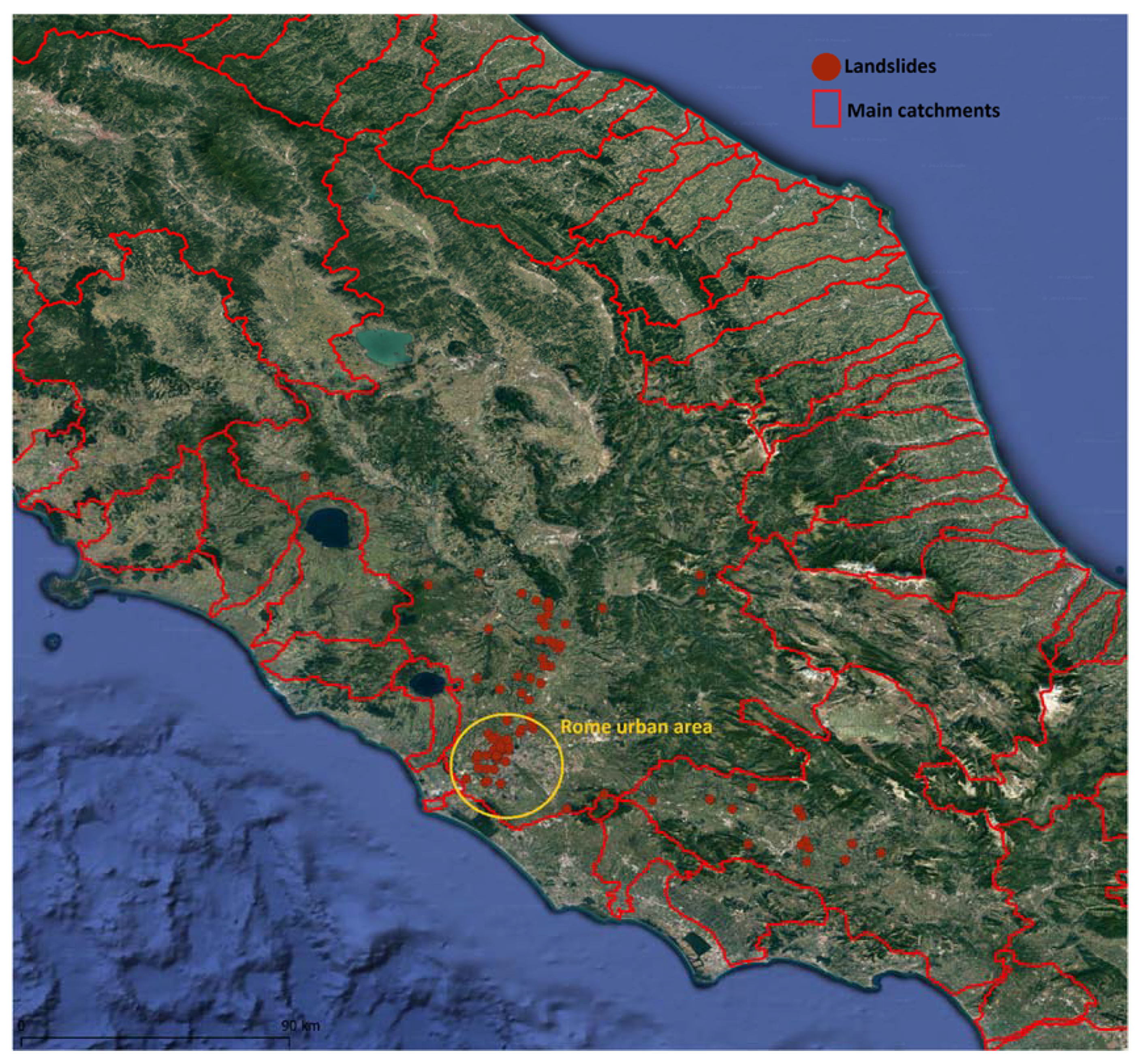
Figure 1. Location of landslide events (brown circles) reported during the event in the Lazio Region Civil Protection Report and press releases. The yellow circle indicates the urban area of Rome. For a better localization of each phenomenon, the file named “Domain.kmz” for the visualization on GoogleEarth© is provided in the Supplementary Material.
Hydrology 09 00139 g001
Figure 2. Location of flood events (cyan circles) reported during the event in the Lazio Region Civil Protection Report and press releases. The yellow circle indicates the urban area of Rome. For a better localization of each phenomenon, the file named “Domain.kmz” for the visualization on GoogleEarth© is provided in the Supplementary Material.
Hydrology 09 00139 g002
Figure 3. Geopotential height at 500 hPa (shades) and sea level pressure (white isolines) from 30 January to 4 February 2014 over Europe. Source: Global Forecast System Analyses Url: www.wetterzentrale.de (accessed 29 July 2022). For a better visualization of each panel, please refer to the document provided in the Supplementary Material, which contains a wide view of each single panel from page 16 to page 21.
Hydrology 09 00139 g003
Figure 4. Skew-T diagram related to the sounding on Pratica di Mare carried out at 00 UTC on 31 January 2014.
Hydrology 09 00139 g004
Figure 5. Accumulated rainfall from 30 January to 5 February 2014. The precipitation field is spatialized over the geographical domain starting from punctual range gauge data. Blue numbers indicate the location of the Riano (no. 1) and Ottavia (no. 2) rain gauges, where rainfall maxima were recorded. The image is taken from the Dewetra platform [27] (Accessed 31 July 2022).
Hydrology 09 00139 g005
Figure 6. Geographical location of dams and hydrometric sensors. Gauge pinpoints are colored according to their critical status. Red lines indicates main basins boundaries. For a better and interactive visualization, a. kmz file, named “Domain.kmz” is provided with the Supplementary Material.
Hydrology 09 00139 g006
Figure 7. BDD index daily maps for relevant days of the weather event.
Hydrology 09 00139 g007
Figure 8. CAI index daily maps for relevant days of the weather event.
Hydrology 09 00139 g008
Figure 9. LAI index daily map for 31 January 2014.
Hydrology 09 00139 g009
Table 1. Main hydrological processes parameterized in the CHyM model and their references.
Physical ProcessCalculation Method
Surface runoffKinematic wave approximation of the shallow water (Lighthill and Whitam, 1955)
EvapotranspirationFunction of the reference evapotranspiration according to Thornthwaite and Mather, 1957)
MeltingTemperature index (Pellicciotti et al., 2005)
Infiltration and percolationConceptual model from Overton (1964)
Table 2. BDD, CAI and LAI thresholds for Ordinary (OS), Moderate (MS) and High Stress (HS).
OSMSHS
BDD3 mm/h6 mm/h11 mm/h
CAI30 mm/day60 mm/day110 mm/day
LAI190 mm/day360 mm/day540 mm/day
Table 3. Statistical scores used to evaluate the indices timing, compared to the hydrometric level temporal evolution.
ScoreUnit of MeasureDescription
Lag Time Peak (LTP)hoursIt compares two timeseries of two different variables (signals) and investigates the synchronicity of the absolute maximum.
Relative Lag Time Peak (RLTP)/It is the LTP divided by the concentration time in the river section where the score is calculated [44]
Correlation Time Delay (CTD)hoursIt represents the value of the lag time (hours) needed to shift one timeseries toward the other, in order to maximize their correlation [45]
Derivative Dynamic Time Warping (DDTW)/It estimates the deformation (stretch or compress) needed to be applied to one timeseries, respect to a reference one, in order to maximize their fit. The calculation is applied to the local derivative of the two timeseries [46].
Table 4. Contingency table scores of BDD and CAI over the three investigated catchments.
BDD INDEXCAI INDEX
APODFARAPODFAR
TIBER RIVER BASIN0.900.480.060.810.030.05
Upper course0.980.830.220.960.190.09
Middle course0.940.570.000.880.040.00
Lower course0.740.400.080.520.010.00
NORTHERN LAZIO BASINS0.921.000.000.961.000.80
LIRI-GARIGLIANO BASIN0.920.000.000.931.000.00
Table 5. Timing scores of BDD and CAI indices.
Bdd IndexCai Index
LTPRLTPCTDLTPRLTPCTD
TIBER RIVER BASIN−4.0−0.71.4−10.6−1.21.0
Upper course−1.2−0.41.8−7.4−0.91.1
Middle course−11.6−1.51.1−16.5−2.11.1
Lower course0.6−0.21.2−8.1−0.61.0
NORTHERN LAZIO BASINS4.80.50.8−0.50.00.8
LIRI-GARIGLIANO BASIN1.60.40.8−7.1−0.50.8
Table 6. DDTW of BDD and CAI indices.
BDDCAI
TIBER RIVER BASIN0.120.16
Upper course0.200.25
Middle course0.130.22
Lower course0.040.01
NORTHERN LAZIO BASINS0.190.15
LIRI-GARIGLIANO BASIN0.010.26
Publisher’s Note: MDPI stays neutral with regard to jurisdictional claims in published maps and institutional affiliations.