Integrating Drone Technology into an Innovative Agrometeorological Methodology for the Precise and Real-Time Estimation of Crop Water Requirements

Abstract

Precision agriculture has been at the cutting edge of research during the recent decade, aiming to reduce water consumption and ensure sustainability in agriculture. The proposed methodology was based on the crop water stress index (CWSI) and was applied in Greece within the ongoing research project GreenWaterDrone. The innovative approach combines real spatial data, such as infrared canopy temperature, air temperature, air relative humidity, and thermal infrared image data, taken above the crop field using an aerial micrometeorological station (AMMS) and a thermal (IR) camera installed on an unmanned aerial vehicle (UAV). Following an initial calibration phase, where the ground micrometeorological station (GMMS) was installed in the crop, no equipment needed to be maintained in the field. Aerial and ground measurements were transferred in real time to sophisticated databases and applications over existing mobile networks for further processing and estimation of the actual water requirements of a specific crop at the field level, dynamically alerting/informing local farmers/agronomists of the irrigation necessity and additionally for potential risks concerning their fields. The supported services address farmers’, agricultural scientists’, and local stakeholders’ needs to conform to regional water management and sustainable agriculture policies. As preliminary results of this study, we present indicative original illustrations and data from applying the methodology to assess UAV functionality while aiming to evaluate and standardize all system processes.

1. Introduction

As a result of the environmental impact factors and the growing demands on food production and consumption, combined with the global market demand to keep merchandise prices low, the modern agricultural industry faces a major challenge [1,2]. There is greater urgency than ever before for producers, farmers, and agronomists around the world to improve the management of their agricultural practices on farms in response to the reduction in their budgets through the optimization in water-saving and farm inputs and, at the same time, maintain high product quality [3]. Future water requirements, combined with limited or bad quality water resources and requirements to adequately meet a growing population’s increasing nutritional needs, require improved crop yields and productivity and increased irrigated land, even in the planet’s arid areas.

Globally irrigated agriculture delivers 40% of the food production and consumes 70% of the available water [1,4]. Therefore, irrigation scheduling is an important tool for improving the efficient use of irrigation water. Recently, several new sensors and emerging technologies, such as the Internet of things (IoT), have been developed and applied in precision agriculture for the management of available water resources and the biometeorological monitoring of plants and soil [2,5]. These provide significant potential in precision agriculture (PA) and smart farming since it has a direct impact on improving the management of irrigation systems and enabling a long-term increase in productivity [6]. Nowadays, the scientific community focuses not only on estimating the duration of irrigation but also on the accurate calculation of actual needs (actual evapotranspiration (Eta)) regarding the water required by each crop [7]. This trend is contrary to the general tendency of determining the maximum rate of evapotranspiration of the crop (ET_C) in large estimation time steps. Additionally, the effect of the vegetation surface (temperature, physical characteristics, etc.) on the precise estimation of actual evapotranspiration values is also one of the main issues of research [7].

Earth observation data with variations in spectral, spatial, and temporal characteristics have been widely used for vegetation mapping and crop water stress monitoring [8,9,10,11]. Traditional remote sensing methods place remote sensors over crop fields or use aircraft and satellites where the appropriate fixed position or the temporal and spatial resolution significantly bounds their utility for PA [12,13,14]. However, freely available optical-sensors-based imagery is often unsuitable for monitoring crop water stress at the farm level due to the poor revisiting times and coarse spatial resolutions. At the same time, the higher accuracy data are too expensive [15,16]. Furthermore, these data are typically unavailable or not useful on cloudy days [2,17]. Nevertheless, for decades, a lot of studies were undertaken to monitor the crop water stress index using satellite- and aerial-based instruments in several crops, such as those of Rud et al. [18] and Cucho-Padin et al. [19] in potato fields, Veysi et al. [20] and Lebourgeois et al. [21] regarding sugarcane, da Silva et al. [22] regarding melon, Sepulcre-Cantó et al. [23] in olive orchards, and Gutiérrez et al. [24] regarding vineyards.

The synergistic utilization of innovative UAV advanced high-precision thermal cameras and other infrared sensors have enhanced the usefulness of these systems to monitor water statuses [25,26]. As a result, numerous studies have researched several different crops to evaluate the crop water stress conditions, such as those of Zhang et al. [16,27], Yang et al. [28], Gago et al. [12], Gonzalo-Dugo et al. [29], Bellvert et al. [30], Berni et al. [31], Matese et al. [32], and Santesteban et al. [33]. However, the process of calibrating and processing thermal images takes a long time to give the final decision on whether to irrigate. In addition, this process involves more empiricism. Therefore, even a high-precision thermal camera could not be described as a useful tool for everyday use on extensive arable land. The CWSI can be determined using at least two different methodologies: the theoretical model proposed by Jackson et al. [34], which is based on meteorological models, and the empirical model proposed by Idso et al. [35], which has achieved considerably more popularity due to the limited data requirements [8,16]. Due to its simplicity and requiring only three variables to be measured, this practical approach has received much attention in the literature. However, it received criticism concerning its inability to account for temperature changes due to radiation and wind speed [36]. The theoretical method is more complicated because it requires these two additional variables to be measured to evaluate the aerodynamic resistance. Moreover, given the assumed net radiation and wind speed, the theoretical approach to calculating the CWSI promises to improve the estimation of plant water trends [36]. Considering the above, the methodology for estimating the CWSI coefficients is based mainly on the theoretical approach. For this purpose, all the necessary sensor equipment was installed for the CWSI calibration stage for three crops independently.

The GreenWaterDrone (GWD) project proposed a pilot implementation of an innovative and autonomous system (onboard micrometeorological station) that identifies a farmer’s real-time irrigation needs through the CWSI to estimate each crop’s water status. The direct estimation of the CWSI is based on spatial data that is remote and directly from the field and is based mainly on the infrared temperature of the crop canopy. Even in the recent (2021) literature, but also in previous years, the calculation of the CWSI with direct spatial measurements of the temperature of the crop canopy has never been proposed or adapted [37,38,39,40,41,42,43]. Such measurements are constantly achieved indirectly through thermal images. The raw data and thermal images from the infrared camera were also used for comparison and calibration purposes. The use of the spatial measurements of canopy temperature, air temperature, and relative humidity from sensors incorporated into an unmanned aerial vehicle (UAV) may be a global novelty. This study aimed to present the new methodology and the equipment used in the assessment of crop water stress by presenting preliminary results from the initial stages of a pilot implementation in a potato cultivation field at the farm scale.

2. Description of the GWD Concept

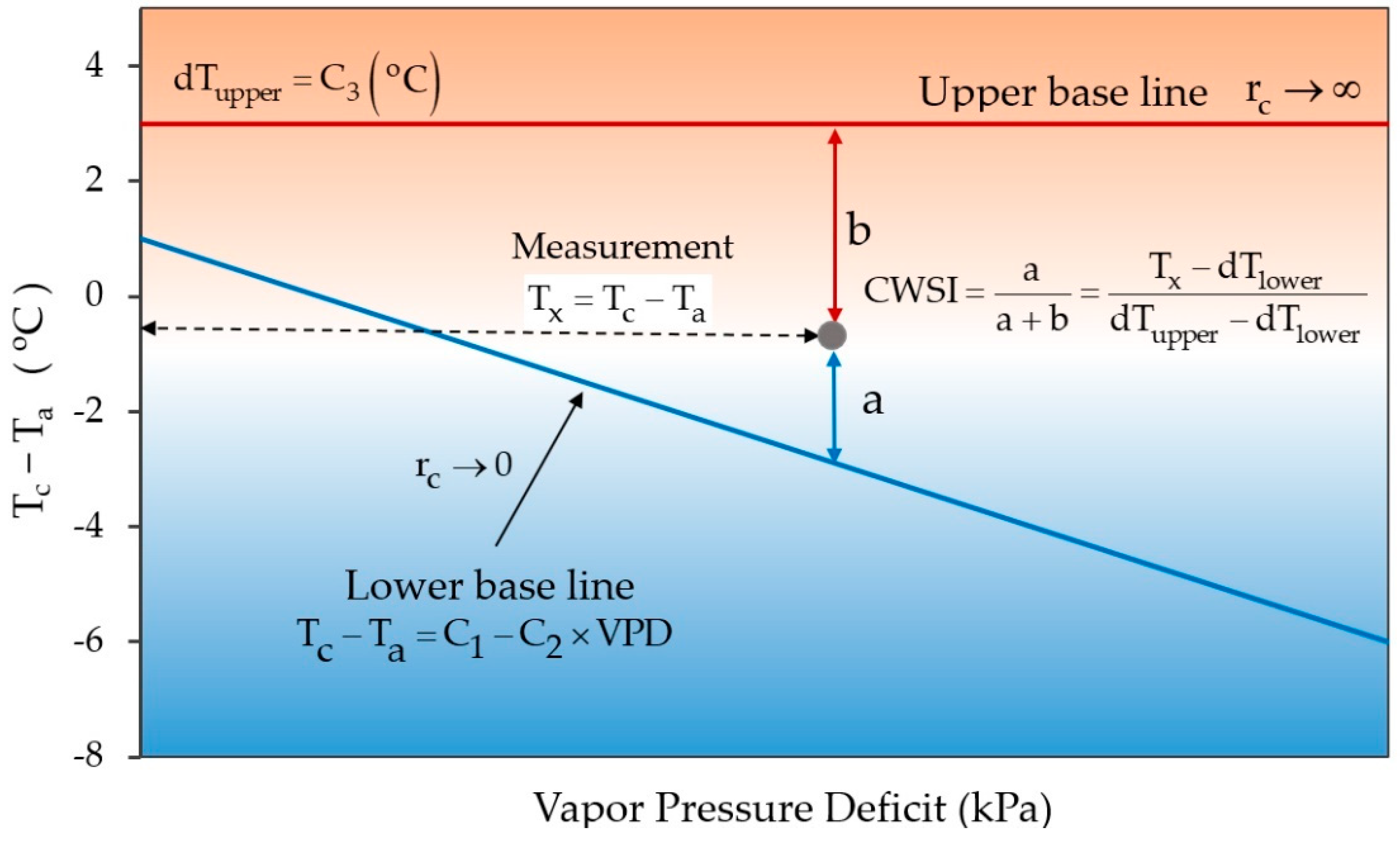
2.1. CWSI—Empirical and Theoretical Approaches

CWSI is a measure of the relative transpiration rate that occurs from a crop and is found by using the canopy temperature and the vapor pressure deficit as relevant variables. The latter measure is related to the atmospheric dryness over the crop. The CWSI approach [34] utilizes the energy balance theory that separates the net radiation over the canopy from the sensible heat (thermal content of the air) and latent heat that is consumed for transpiration. The energy balance considerations show how the difference between the canopy and air temperatures (T_c − T_a) is related to the vapor pressure deficit (VPD), and the flux density of the net radiation (R_net) presents a theoretical basis for the CWSI.

When the plant canopy is fully transpiring, the leaf temperature is some degrees below the overlying air layer temperature and the CWSI is equal to 0 (stomata are closed). Conversely, as the transpiration decreases, the leaf temperature rises and can reach some degrees above the overlying air temperature. When the canopy is no longer transpiring, the CWSI is equal to 1. Because of the scatter in the measured canopy minus air temperature vs. the vapor pressure deficit, the crop does not need to be watered until the CWSI reaches 0.1 to 0.15. For example, for eggplant crops, it could be possible to use values of CWSI between 0.18–0.20 for high and good quality yields. Irmak et al.’s [44] work showed that when the CWSI value exceeds more than 0.22, this resulted in a decreased corn grain yield. Determining the temperature upper line (maximum stress) is not a simple process for any crop. However, this empirical approach has attracted much interest due to its simplicity. It requires measuring the canopy temperature (T_c), air temperature (T_a), and the vapor pressure of the atmosphere’s deficit (VPD).

After the empirical approach suggested by Idso et al. [35], a theoretical method for calculating the CWSI was presented. The index’s practical estimation is calculated by determining the relative distance between the lower baseline representing the soil water adequacy conditions in the rhizosphere (no stress) and the upper baseline representing the crop’s maximum water stress (no transpiration by plants; Figure 1).

The two lines (blue and red) presented in Figure 1 are suitable for assessing a crop’s water status during the warm seasons of the year when irrigation is required. These lines are the result of local calibration and concern the specific crop that is studied each time. The lower baseline is determined for the crop by plotting (T_c − T_a) against the local VPD after a significant watering. A sufficient number of measurements (10 min time step) around midday were taken for the precise estimation of the canopy temperature (T_c). The canopy’s temperature sampling must be repeated several times, including measurements under dry and wet atmospheric conditions. This results in a full range of measures representing the lower regression line for a wide range of value pairs (Τc − T_a vs. VPD). The upper baseline could be determined after cutting the plant and taking the canopy temperature the next day, as the plant no longer transpires. The theoretical procedure requires a measurement of the net flux density of the radiation (R_n) and an aerodynamic resistance factor, in addition to the air temperature and relative humidity of the air that is required by the empirical approach [36].

The theoretical development of the CWSI is based on the well-known equation of energy balance of the surface ($R_n-G=H+\lambda E$), where $R_n$: net radiation, G: soil heat flux, H: sensible heat flux, and $\lambda E$: latent heat flux of evaporation. All the terms are in ${\mathrm{Wm}}^{-2}$. The terms H and $\lambda E$ are expressed in Equations (1) and (2), which are based on two assumptions (see [36,45,46,47]):

$$H=\rho C_p\left(T_c-T_a\right)/r_a$$

(1)

$$\lambda E=\left[\rho C_p\left(e_s-e_a\right)\right]/\left[\gamma \left(r_a+r_c\right)\right]$$

(2)

where $\rho :$ density of air (kg m⁻³), C_p: specific heat moist air (1.013 kJ kg⁻¹ °C⁻¹), $T_{c }$: canopy temperature (°C), $T_a$: air temperature (°C), $e_s$: saturated vapor pressure (kPa), $e_a$: actual vapor pressure (kPa), $\gamma :$ psychrometric constant (kPa °C⁻¹), $r_a$: aerodynamic resistance (sm⁻¹), and $r_c$: bulk surface resistance (s m⁻¹).

Clothier et al. [48] showed that the soil heat flux estimation can be calculated from R_n measurements with reasonable accuracy. The ratio G/R_n for full canopies (more than 45 cm) is nearly constant at 0.1. Thus, the soil heat flux does not contribute significantly to the energy balance above the canopy. Taking $G=0.1R_{net}$ the equation becomes $I_c{R}_n=H+\lambda E$, where $I_c$ = 0.9 is an interception coefficient.

$$T_c-T_a=\frac{r_a{I}_c{R}_n}{\rho C_p}\cdot \frac{{\gamma }^{\ast }}{\Delta +{\gamma }^{\ast }}-\frac{VPD}{\Delta +{\gamma }^{\ast }}$$

(3)

where γ* (kPa °C⁻¹) is the modified psychrometric constant and VPD is the vapor pressure deficit.

Equation (4) represents the slope of the saturated vapor pressure relation:

$$\Delta =\left(e_{s_C}-e_s\right)/\left(T_c-T_a\right)$$

(4)

where $e_{s_C}$ and $e_s$ represent the saturated vapor pressure of the canopy temperature and the air temperature, respectively.

The upper limit $T_c-T_a$ is determined when the canopy resistance tends to infinity $\left(T_c-T_a\to \infty \right)$ and Equation (3) becomes

$${\left[T_c-T_a\right]}_{ul}=\frac{r_a{I}_{cu}{R}_n}{\rho C_p}$$

(5)

The lower limit, determined by setting the bulk surface resistance $r_c=0$, is

$$T_c-T_a=\frac{r_a{I}_{cl}{R}_n}{\rho C_p}\cdot \frac{\gamma }{\Delta +\gamma }-\frac{VPD}{\Delta +\gamma }$$

(6)

Thom and Oliver [49] proposed an effective aerodynamic resistance $r_{ae}$ that represents a semi-empirical equation for $r_a$:

$$r_{ae}=4.72\mathrm{l}{\left\{\ln \left[\left(z-d\right)/z_o\right]\right\}}^2/\left(1+0.54u\right)$$

(7)

The crop water stress index can be estimated using the equation below:

$$CWSI=\frac{\left(T_c-T_a\right)-{\left(T_c-T_a\right)}_{ll}}{{\left(T_c-T_a\right)}_{ul}-{\left(T_c-T_a\right)}_{ll}}$$

(8)

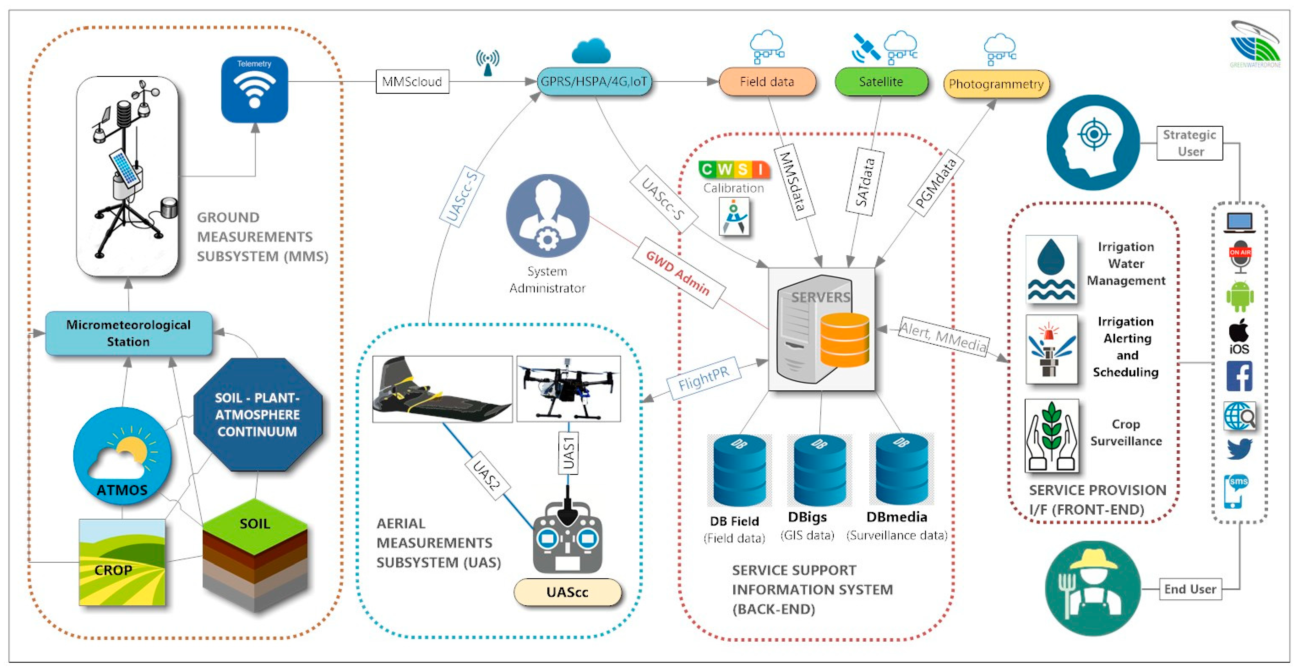
2.2. Structure and Architecture of the GWD Project

The GreenWaterDrone system is functionally and physically divided into four subsystems, as follows (Figure 2):

• The ground measurements subsystem (MMS), which is applied only during the calibration phase, consists of micrometeorological stations and their integrated/peripheral sensors, which are required to collect microclimatic and soil measurements of the crop field. Data collected from a station is used to calibrate and approximate the CWSI of a specific crop under the local climatic regime for one growing season. Data is communicated to the system over available mobile WAN infrastructures (2/3/4 G, IoT).
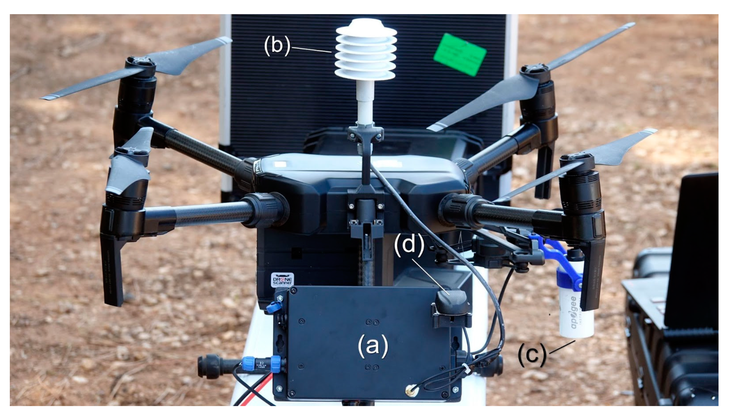
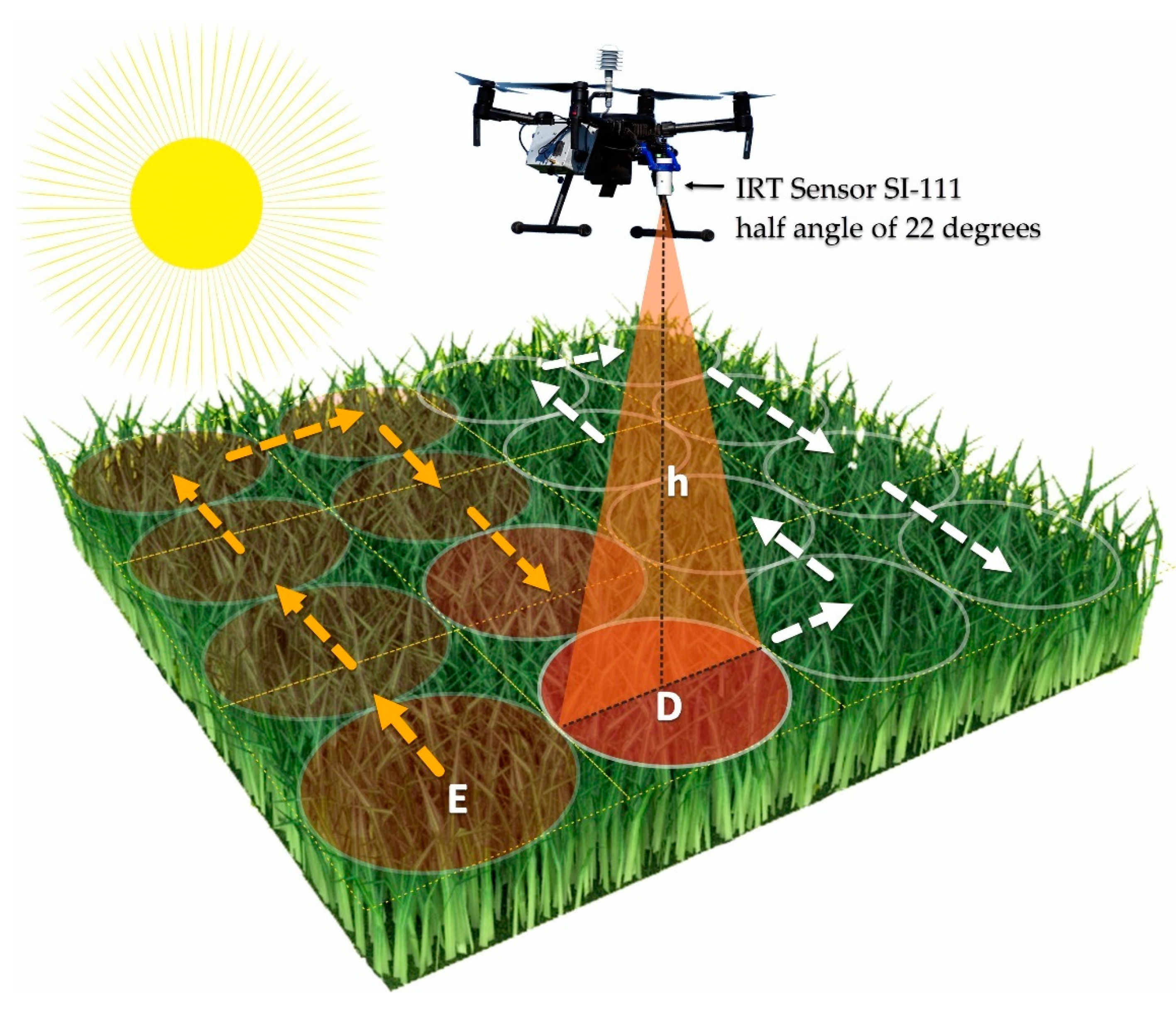
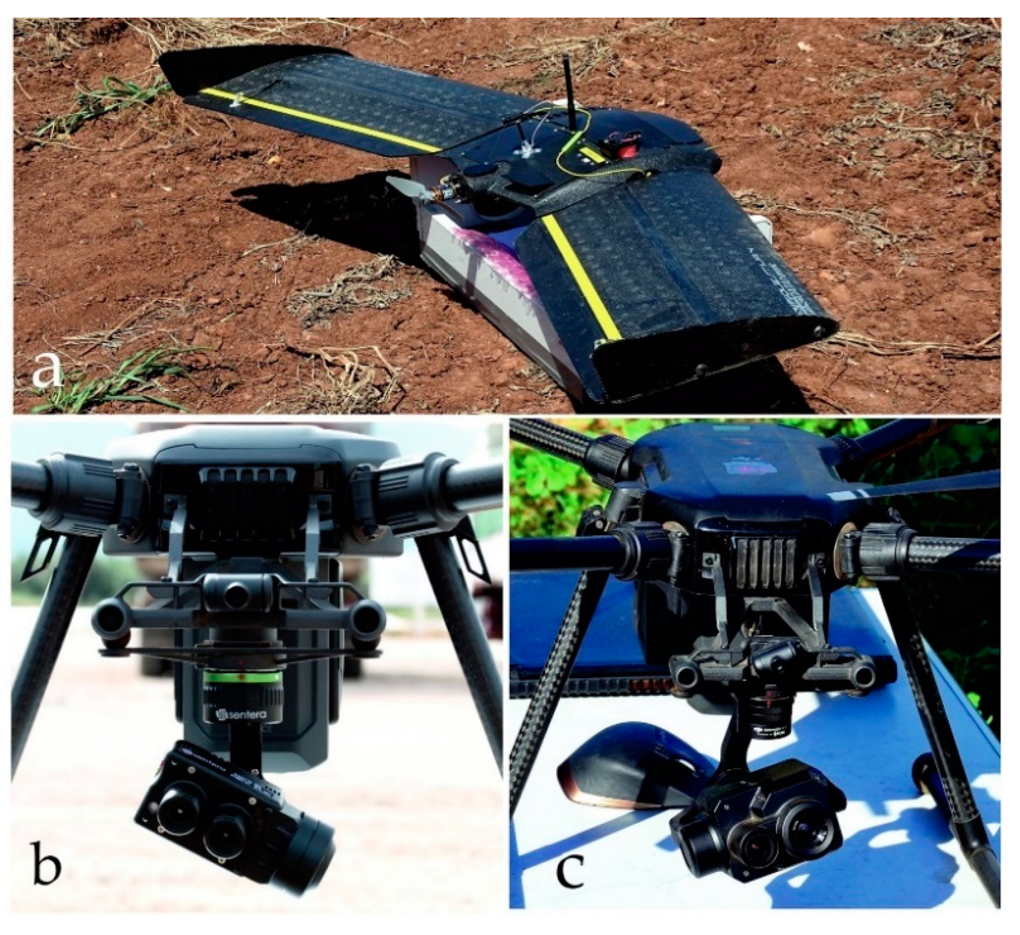
• The aerial measurement subsystem (UAS) consists of two types of UAVs. A quadcopter platform UAS1 uses an autonomous microstation to collect raw spatial data from the crop foliage and environment (infrared temperature, air temperature, relative humidity, accurate coordinates, and elevations). A fixed-wing platform UAS2 is required to collect thermal, multispectral, and photogrammetry images over large crop areas. Field data collected by the UAS is communicated to the system over available mobile WAN infrastructures (2/3/4 G, IoT). Both scheduled (e.g., during calibration and normal operation) and emergency (e.g., extreme weather conditions) flights are managed by the GWD System Administrator via the FlightPR interface.
• The service support information system (BackEnd) implements the crop data management necessary for the storage, classification, management, and updating of field measurements, empirical irrigation data, spatial and crop quality data, field status multimedia, end-user preferences, and interfaces with external services (satellite imagery, photogrammetry applications). In addition, it interconnects and supports all other subsystems and is responsible for providing the services of the system (alerting and multimedia content) to all types of supported end users.
• The service provision I/Fs (FrontEnd) includes appropriate web interfaces of the system to predefined types of GWD users, such as plain (farmers/agronomists), group (partnerships), and strategic (local/regional authorities) end users, with graded access to the three supported applications through different devices (PCs, smartphones, etc.) and relevant GUIs.

The GWD system supports the following applications to provide a comprehensive irrigation management and field surveillance framework to both the plain and strategic end users that are targeted:

• Irrigation alerting and scheduling (IRRas): The plain end user (farmer/agronomist/farmer partnership) receives alerts in near real time regarding the short-term need to irrigate (or not) a specific crop based on CWSI calculations and empirical irrigation scheduling.
• Crop surveillance (CS): The plain end user (farmer/agronomist/farmer partnership) can view on-demand, multimedia content (e.g., photos/video relating to crop condition) of a field or receive alerts in near real time regarding the availability of synchronous video/photos of his crop in the case of a natural disaster or a security issue triggering an emergency drone flight.
• Irrigation water management (IRRmgt): The strategic user (agricultural institute, local/regional authorities) may select zones (clusters) on a graphical interface with a map of the area covered by the GWD system (effectively calibrated crops in the area) and obtain irrigation requirements for specific crop patterns and periods, thus enabling the implementation of scenarios for future irrigation water policies.

3. Case Study—Materials and Methodology

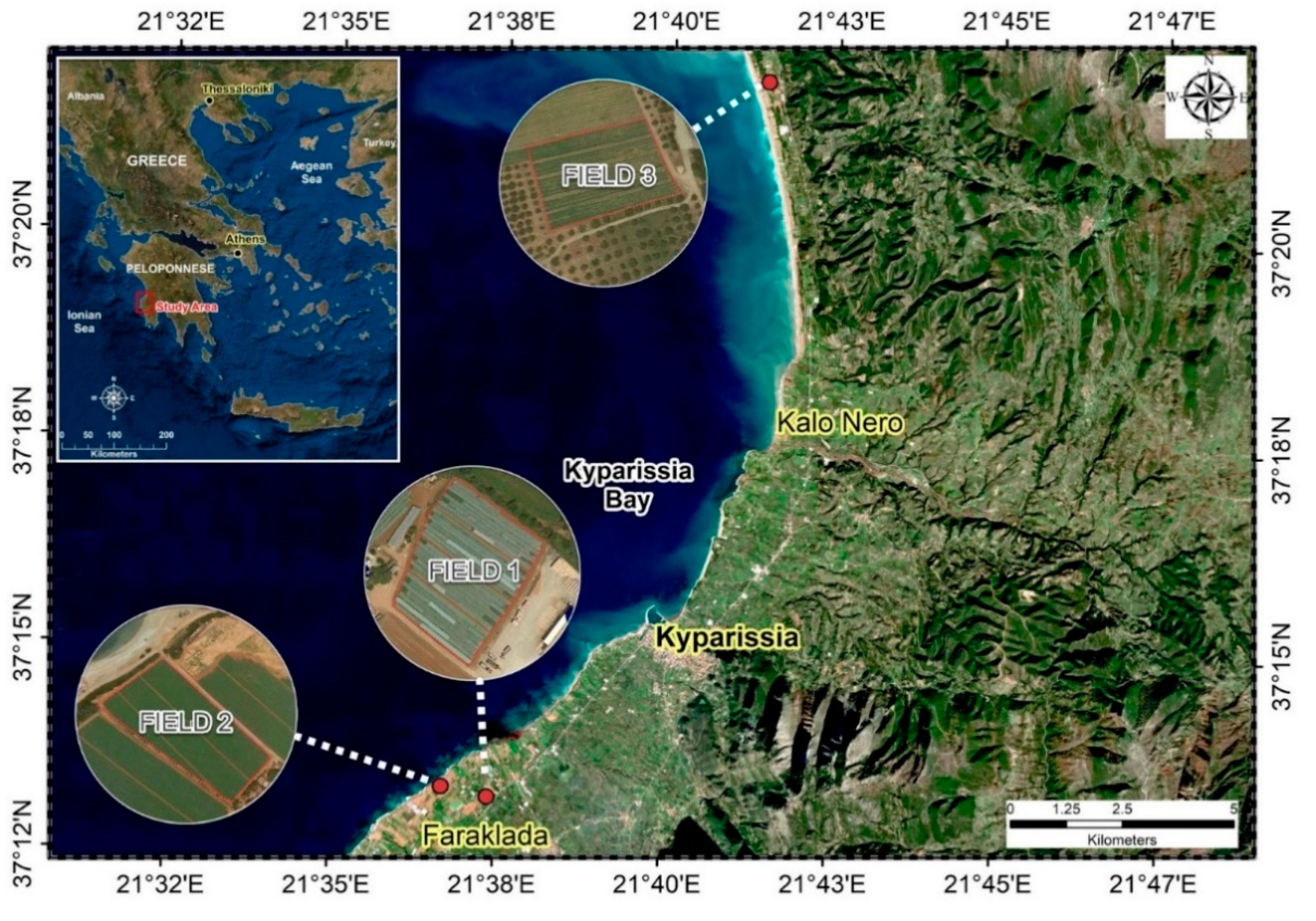
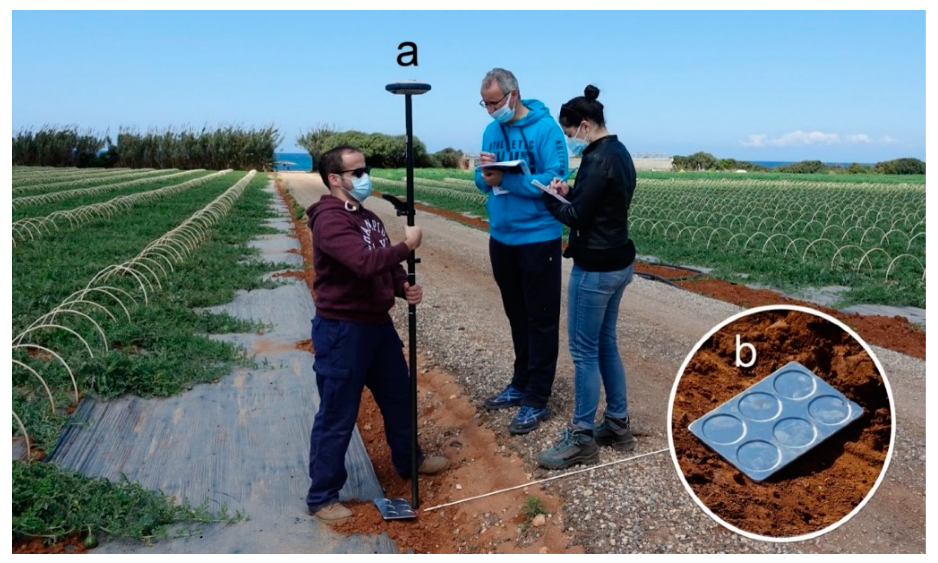
3.1. Study Area

The study area was situated in the prefecture of Messinia (western Peloponnese), close to the city of Kyparissia in the Municipality of Trifilia (Figure 3). Based on long-term data obtained from the nearby station of Kalamata (37.07° N, 22.10° E, alt. 8 m a.s.l.) over the last century, the broader area has a humid climate according to Thornthwaite’s climate classification system (UNEP 1992), which has, however, become drier nowadays compared to the past, as seen via the decreasing aridity index [50] values from 0.88–0.89 in the previous climatic periods (1900–1930 and 1930–1960) to 0.85 in the period 1960–1997 [51].

The experimentation was conducted in three fields with three different crops that are representative of the area, i.e., potato, watermelon, and tomato, which were utilized for the validation procedure of the GWD project methodology (Figure 3). Indicatively, in this work, potato field 2 (Solanum tuberosum; 1.25 hectares; 37°13′20.65″ N, 21°36′41.51″ E, alt. 1 m a.s.l.) was used throughout the next sections for demonstrating the preliminary results of the different imaging used in the project and GWD methodology validation during the 2019 growing season. The potato crop was selected by considering its relatively high water requirements, with its maximum in the hot and dry summer period, and the critical susceptibility of potato plants to water stress, which is attributed mainly to their relatively shallow root system (Figure 4a) [18]. The field had a small slope of 0–3% and a clay loam surface soil layer (0–20 cm depth), becoming sandy clay loam further down (20–60 cm depth; Figure 4b).

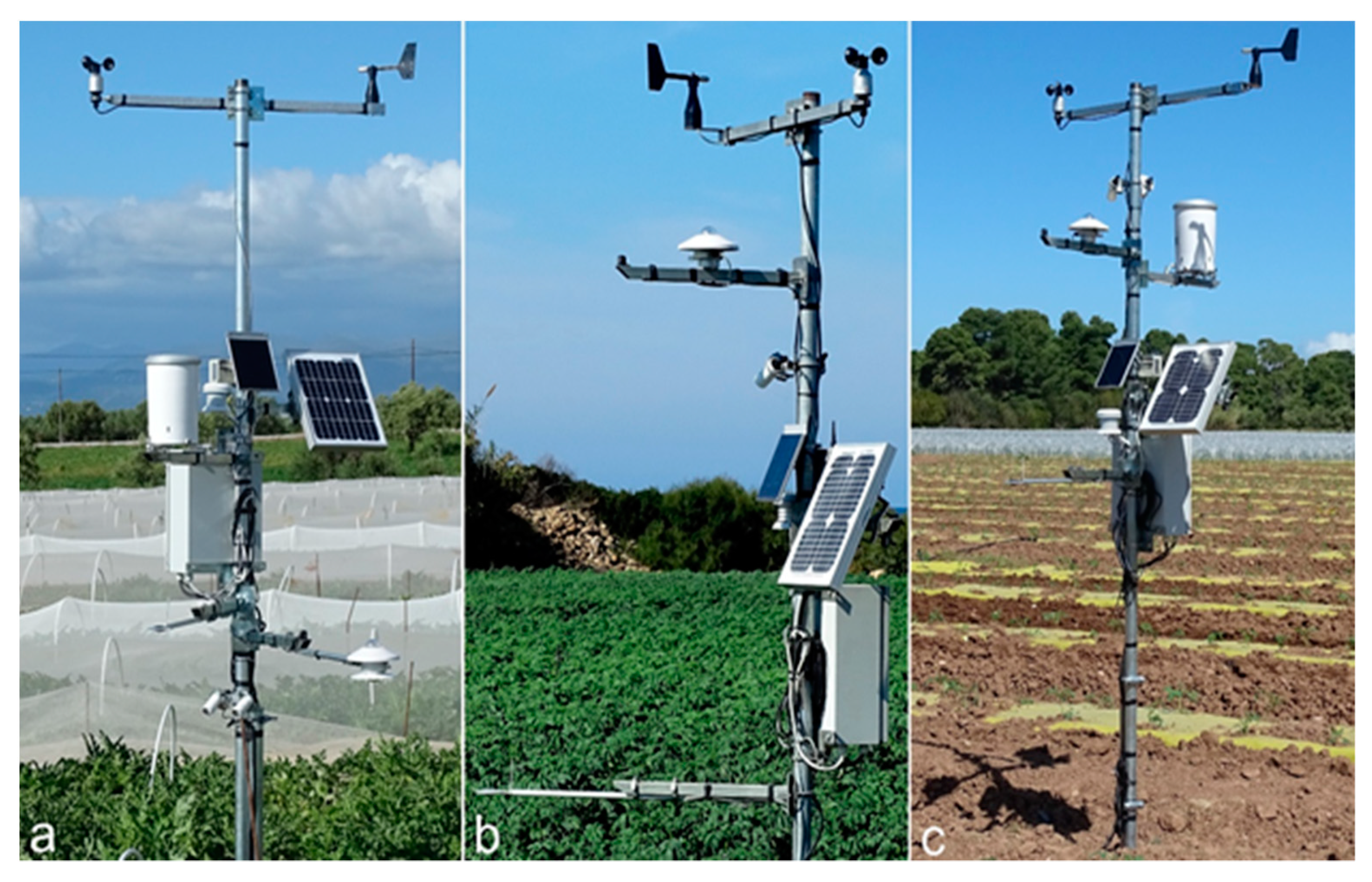
3.2. Ground Micrometeorological Station

Three automatic micrometeorological stations were installed in the middle of the fields (Figure 5) for observations of the upper atmospheric layer of the crops and measurements within the soil profile (at the root zone). This was an indispensable condition for the accurate estimations of CWSI and the determination of all the biophysical attributes of the cultivations during all stages of the growing season. This ground-based measuring system composed the core of the calibration for estimating the CWSI of each crop, which was the basis for determining the real-time irrigation needs according to the methodology proposed by the GWD project.

3.2.1. Measurements above Crops

The three ground micrometeorological stations (GMMS) were equipped with the following sensors:

• A high-precision miniature air temperature (T) and relative humidity (RH) sensor model EE08 (Elektronik Ges.m.b.H, Austria) working over a wide range was installed at a 2 m level.
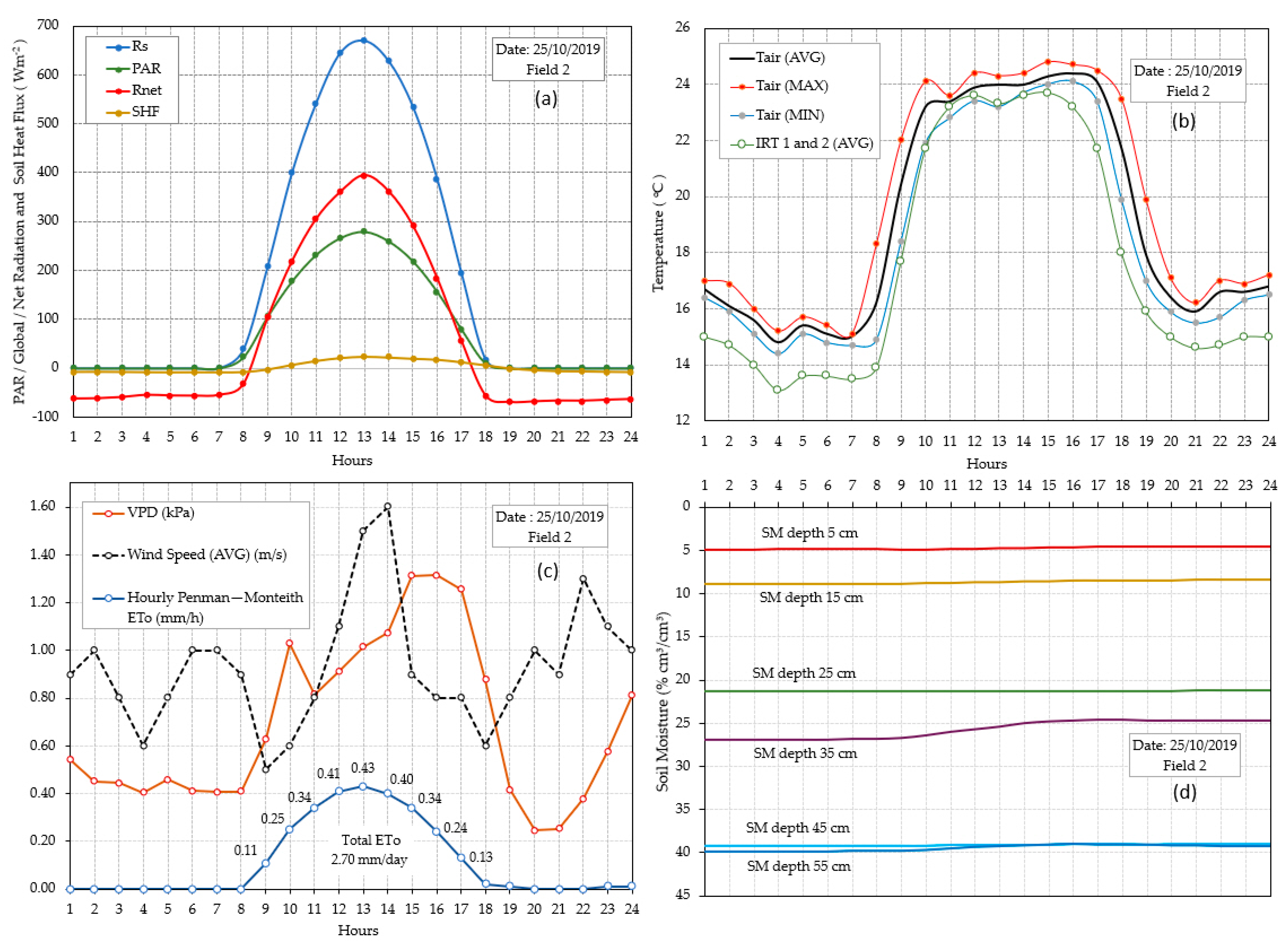
• The LPPYRA02 fitted on stations 2 and 3 is a spectrally first-class pyranometer that measures the shortwave (Rs) solar radiation flux density on a flat surface (in Wm⁻²; global irradiance, sum of direct and diffuse radiation).
• A pyranometer following ISO 9060:2018 with the criteria of the WMO “Guide to Meteorological Instruments and Methods of Observation.” An albedometer LP PYRA 05 (Delta OHM, Italy) was fitted on station 1 and measured the global radiation (in Wm⁻²) and the albedo of any surface. It was manufactured incorporating two LPPYRA02 pyranometers into only one body.
• Net radiation pyranometer (RNET LP NET 07 Delta OHM, Italy) for the net flux density measurement (Rn) passing through a surface across the near-ultraviolet and the far-infrared spectral ranges.
• Photosynthetically active radiation sensor PAR (QUANTUM SENSOR Model SQ-100-SS APOGEE, Italy) that measured the total radiation across the range of 400–700 nm expressed as photosynthetic photon flux density (in µmol m⁻² s, equal to μE m⁻² s).
• Two tipping bucket rain gauges, model HD2015 and model HD2015 (Delta OHM, Italy), for precipitation measurements in millimeters (Pre) were installed on stations 1 and 3. It should be noted the distance between meteostations 2 and 3 was 15 km along the north–south axis, while the distance between meteostations 1 and 2 was 1 km.
• Cup anemometers for horizontal wind speed (WS) measurement (in m/s; model 4.3519.00.167 Thies GmbH & Co, Germany) and wind direction (WS) sensor (in degrees; model 4.3140.51.010 Thies) were installed on the mast at a height of 3.4 m for the three meteostations.

Given the importance of measuring the temperature of the plant foliage (canopy) remotely, reliable infrared radiometer sensors were crucial for achieving the program’s objectives. The model SI-111-SS (Apogee, Berkeley, CA, USA), which is an unamplified analog sensor with a standard field of view, was selected to measure the canopy temperature. The response time of the sensor is 0.6 s, with a measurement repeatability of less than 0.05 °C, and the calibration uncertainty is 0.2 °C. The spectral range of the measurement is between 8 and 14 µm, that is, the atmospheric window. The sensor has a 22° half-angle field of view. The placement height and the angle formed between the mast with the longitudinal axis of the infrared thermometer determine the elliptical area of measurement (in m²) of the surface of the dense canopy.

Moreover, portable infrared thermometers (Model MI-210 Apogee, USA) were used for conducting spatial measurements in all fields’ canopies during the flights of the UAV for calibration and comparative data analysis.

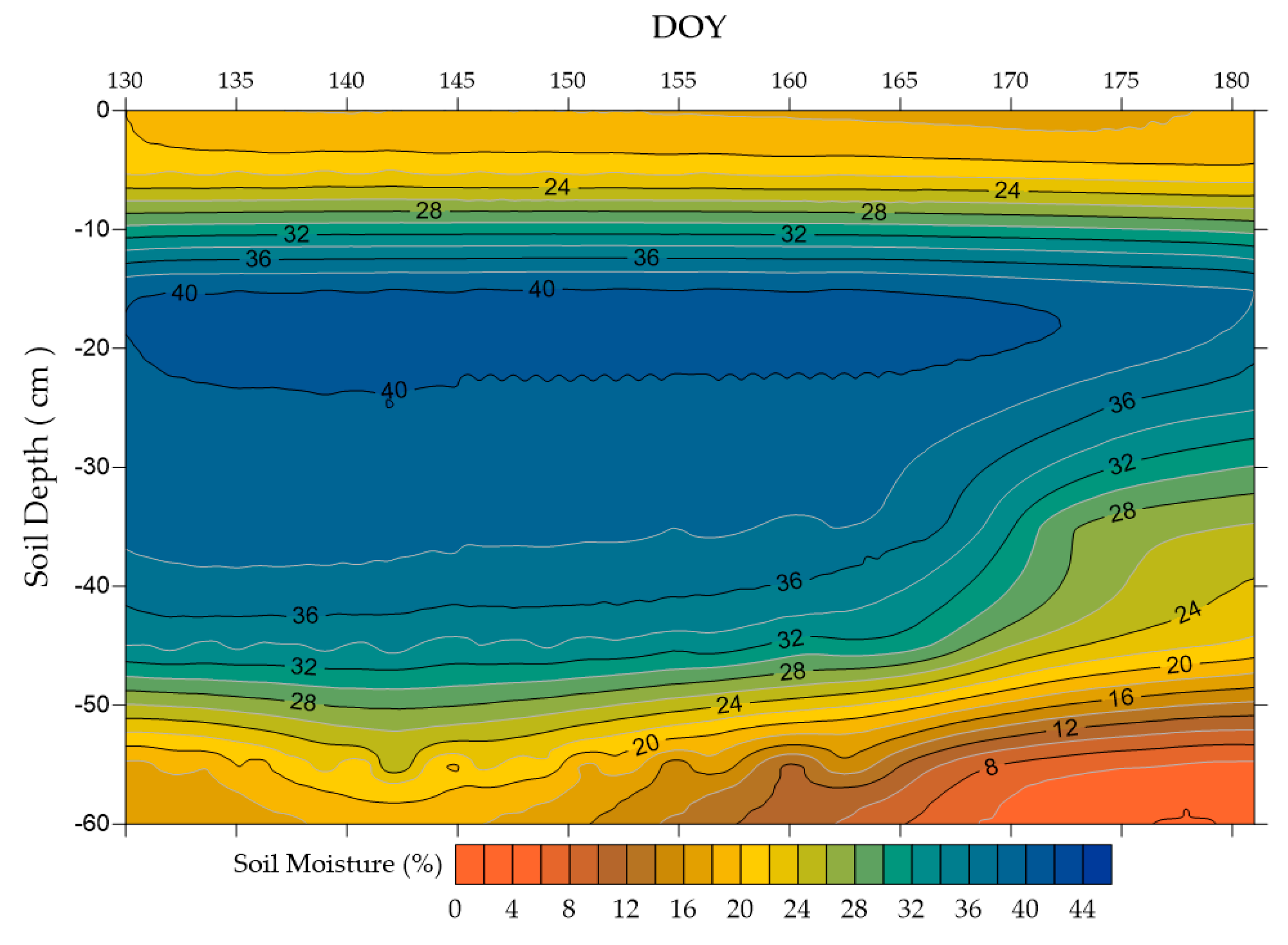
3.2.2. Measurements in the Root Zone

The soil moisture (SMois) (v/v%) and soil temperature (Tsoil) were measured continuously at six soil layers (from 0–10 cm to 50–60 cm in 10 cm intervals) using the Drill and Drop probe (model 00620 Sentek Technologies, Australia). In this way, the actual changes in soil moisture were constantly obtained throughout the depth of the root zone at any time. Furthermore, a soil heat flux plate (HFP01 Hukseflux Thermal Sensor, Netherlands) was installed in the topsoil layer (at a 5 cm depth). Figure 6 graphically shows the soil moisture profile estimated using a geostatistical gridding method (Kriging), which was proven to be useful in many fields. The Kriging method estimates the surface at successive nodes in the grid using only a selection of the nearly closed data points and produces surfaces from irregularly spaced data.

The method efficiently and naturally incorporates anisotropy and underlying trends from a data set by specifying the appropriate variogram model. To create this graph, 1080 daily soil moisture measurements were used from six depths that were monitored in the potato cultivation field for 51 days.

For the detailed fluctuations of the soil moisture of the potato field at depths of 0–10 and 10–20 cm (the two most variable layers), we used 17,284 average values of ten-minute continuous soil moisture measurements. These measurements are shown in Figure 6 and refer to the interval from 10 May to 9 July. The smooth, continuous, and detailed data-collection process, which took place throughout the growing season in the soil profiles, allowed us to accurately estimate the actual evapotranspiration (ETa) from the soil moisture profile in hourly time steps. Moreover, from the observations and characteristics of the plants in all stages (height, LAI, aerodynamic, and surface resistance), in combination with the micrometeorological observations just above the crop (Rs, Rn, albedo, soil heat flux, T, RH), we estimated the crop potential evapotranspiration (ET_c) with satisfactory accuracy. All the above estimates contributed to estimating the crop water stress index (CWSI), both practically and theoretically.

3.2.3. Data Acquisition System and Telemetry

The telemetry unit (model A753 addWAVE GPRS RTU, ADCON (Business Unit of OTT HydroMet GmbH)) provided the possibility of local storage in EPROM Memory for at least half a million measurements. The telemetry unit has an internal rechargeable battery that is charged using a solar panel, which is independent of the one used for the energy needs of the sensors. The duration of operation in normal operation is up to 14 days. According to the GSM standard, the frequency band is 850/900/1800/1900 MHz, and the maximum transmission distance is 36 km. To achieve the maximum accuracy (connecting sensors to a central station unit), especially in the connection of thermocouple sensors (pyranometers, soil heat flux plate) to a central station a unit HD978TR3 (Delta OHM), signal amplifiers were used.

The time step for storing the average data values for each sensor is ten minutes for all stations (144 average values per 24 h). From the ten-minute average values, we obtained and recorded hourly and daily average values for all sensors. All average values from each sensor were found using 4320 reads per 24 h. This means that almost all sensors were automatically excited to give a reading sample every 20 s (3 readings per minute). Of course, this programming considers the response time of each sensor, i.e., the ability of the sensor to respond to two different successive values in time.

3.3. Experimental Design—Unmanned Aerial Vehicle, Cameras, and IR-TH

In the present study, the quadcopter DJI Matrice 200 (DJI Technology Co., Ltd., Shenzhen, China) was used for the measurements of the multispectral and IR-TH data, and the fixed-wing Q100 Datahawk was employed for the photogrammetric mapping of the fields. The quadcopter was selected due to the compatibility of incorporating both multispectral and thermal cameras, and because the flights with infrared sensors require a low flight altitude, low-speed navigation, and high stability, which cannot be achieved with a fixed-wing platform [52]. The accuracy of the system is 10 cm in the vertical and 30 cm in the horizontal, which is considered suitable for PA applications, while at the same time, it offers the possibilities of low, slow, and stable flight. It has significant autonomy and a maximum take-off mass with a large payload (6.14 and 1.61 kg, respectively) and can withstand strong winds (up to 12 m/s), which ensures its smooth operation in demanding flight environments. In addition, the system incorporates an advanced obstacle recognition and avoidance subsystem, which consists of a combination of optical, infrared, and ultrasonic sensors, making the platform one of the safest for flight operations in existence, and incorporates inertial measurement units (IMU) sensors, supporting both automatic, semi-automatic, and manual flights.

The flight planning of the photogrammetric, multispectral, and thermal cameras was conducted with the ground control station software, GS PRO (for the IR), Pix4D (for the thermal camera), Field Agent (for the multispectral camera), and the SkyCircuits Plan and Flight (for the photogrammetric camera), which allow the user to generate a route over a grid path as a function of the field of view of the sensor, flight altitude, flight speed, direction, degree of overlap between images, and ground resolution.

3.3.1. UAV for IR Spatial Row Data Measurements

The DJI Matrice quadcopter was selected to install an autonomous aerial micrometeorological system (MicroStation) consisting of a high-performance data logger (Symetron type Stylitis-12), as well as four sensors: IR radiometer (SI-111-SS Apogee), miniature Thermo-Hygrometer EE08, and an accurate GPS (Figure 7). Through the “Opton 4” Symetron software, the data logger operation was managed and controlled. Furthermore, all the appropriate equations and precalibrated factors for any crop were incorporated into the CWSI estimation software.

The radiation shield plates (which protected the temperature and RH sensors), the watertight box (which protected the data logger), and all the sensors’ mounts were made from lightweight synthetic materials. All these components were designed in a 3D CAD program and printed using a 3D printer in the lab. Particular attention was paid to the placement of the thermo-hygrometer so that it was not affected by the flow of the drone propellers (Figure 7). The vertical positioning of the radiation shield on top of the UAV ensured mild air vortexing and mixing, avoiding the violent airflow from the downside of the drone due to the propellers.

One of the most important parts of the IR instrument sampling workflow was the calculation and design of the most suitable flight planning in order to have the best point samples coverage and complementarity to ideally cover the whole cultivated area. The flight height depends on the sensor type and the characteristics of the crop. For a specific IRT sensor, the visible surface area is a function of height. For the sensor SI-111 that was placed on the UAV in such a way to be vertical to the foliage for a flight height of 4 m (h), the surface area was estimated to be 8.2 m² (E), and the diameter of the circular surface was about 3.2 m (Figure 8).

3.3.2. UAVs for Photogrammetric, Multispectral, and Thermal Measurements

The photogrammetric camera that was used for the present study was the SONY rx 100, with a 20.2 megapixels CMOS lens that has a ground resolution of 3.2 cm/pixel. The camera was adjusted on a fixed-wing Q100 Datahawk UAV (Figure 9a). By processing the images that were produced, an accurate description of the canopy height and a digital surface model (DSM) were created. This information is significant in endeavoring to explore the surface slope inclination and, indirectly, the conditions of drainage and water flow in the soil, as well as the growth conditions of the crop (canopy height and density).

The DSM from UAV image stereo pairs used the structure from motion (SfM) algorithm, which is a photogrammetric technique that was initially developed for archaeological sites [53,54,55]. The algorithm assesses the unknown camera orientations through a comparison of multiple detected image feature points in multiple images. It subsequently produces the 3D structural model of a scene from the overlapping two-dimensional (2D) image sequences that are taken from various spots and orientations [56].

The multispectral camera that was used in the present study was the Sentera AGX710 (12.3 megapixels) multi-spectral sensor with five bands (Sentera Inc., Minneapolis, MN, USA), which cover the blue, green, red, red edge, and near-infrared parts of the electromagnetic spectrum (Figure 9b). Their central wavelengths are 446 nm, 548 nm, 650 nm, 720 nm, and 840 nm, respectively. A 15 cm × 15 cm white reference panel (MicaSense Inc., Seattle, DC, USA) with a 60% nominal reflectance was used for the radiometric correction. UAV imaging was conducted in sunny weather and the period between 11 a.m. and 12 p.m. was chosen for imaging to minimize sunshade. To certify correct image acquisition during the flight, the FieldAgent Mobile App from Sentera was used to plan the flight path and automate the operation of the UAV. A constant flight height was maintained at 30 m and the flight speed was set to 3 m/s. The ground sample distance of the imagery was approximately 1 cm/pixel and a 90% overlap between two images both for side-lap and front-lap was implemented. In total, about 820 images were taken for the experimental field and stacked into a single image for analysis.

Agisoft Metashape Professional (v 1.5.5) was preferred as the Structure for Motion Multi-View Stereo (SfM-MVS) processing software to generate the digital surface model (DSM) and the correspondent normalized difference red-edge index (NDRE) vegetation index.

NDRE is a narrowband greenness VI that was designed to provide a measure of the overall amount and quality of photosynthetic material in vegetation, which is essential for understanding the state of vegetation (photosynthetic capacity and canopy chlorophyll content, structure, and plant health status). NDRE (Equation (9)) was measured by using the NIR and red-edge band (RE; 705 nm), where RE replaces the red band in the widely used normalized difference vegetation index (NDVI) equation. Compared with the NDVI, the NDRE index as a widely used red-edge-based VI was shown to be more resistant to the saturation problem and is more sensitive than the NDVI to chlorophyll content in vegetation [57].

$$\mathrm{NDRE}=\frac{\left({\mathrm{B}}_{\mathrm{NIR}}-{\mathrm{B}}_{\mathrm{RedEdge}}\right)}{\left({\mathrm{B}}_{\mathrm{NIR}}+{\mathrm{B}}_{\mathrm{RedEdge}}\right)}$$

(9)

The final image nominal spatial resolution, expressed as a ground sample distance (GSD), was about 1.2 cm [58].

The final NDRE image ideally demonstrates the plant health status and the existing gaps in the canopy cover and along the cultivation lines, which are important to distinguish and exclude since the reflection from the soil significantly affects the calculation results of the CWSI. Thus, the results of the NDRE image were used to create a binary mask of the soil. Sunlit soil parts were extracted from the image by utilizing a threshold value on a local spatial statistic that characterized the illumination levels [18,59]. This final mask was applied on the co-registered TIR image to produce the thermal product with pixels belonging only to sunlit leaves.

The thermal camera used in the present study was the DJI Zenmuse XT2 (12 MP), which incorporates a high-resolution forward-looking infrared FLIR Tau 2 thermal sensor (FLIR Systems, Wilsonville, OR, USA; resolution 640 × 512 pixels, lens 9 mm; thermal sensitivity of <50 mK) and a 4 K visual camera (1/1.7″ active-pixel CMOS) with a leading stabilization and machine intelligence technology (Figure 9c) [60]. In general, the Zenmuse XT2 camera used in the present study is a very high technological and sophisticated camera that performs radiometric calibration of the acquired thermal images through its advanced digital system, which records the absolute temperature. The calibration of the FLIR camera was performed annually according to the factory specifications, which is carried out by the official supplier by measuring targets with known temperatures and comparing the known and the measured temperatures (e.g., boiling water and melting ice) [16,61]. The thermal lens has a focal length of 19 mm, which avoids previous deformations and obtains rectilinear images. The second lens has a focal length of 8 mm and it also retrieves high-resolution RGB images [62]. The ground sample distance of the imagery was approximately 2 cm/pixel and an 85% overlap between two images for both side-lap and front-lap was implemented. In total, about 382 images were acquired for the experimental field and stacked into a single image for analysis.

UAV thermal imaging was performed in sunny weather from 12:00 to 1:00 p.m. to minimize sunshade and because it has general unique image-acquiring conditions since the maximum temperature differences occur between the soil and vegetation [63,64].

The thermal images acquired by UAV were mosaicked using Pix4D mapper (version 4.5 from PIX4D, Prilly, Switzerland). This software offers an automated SfM procedure, taking a set of images as input and routinely going through the steps of feature identification, matching, and bundle adjustment. The process aligned the images that were acquired by the thermal camera. A polygon mesh was calculated from the dense 3D point, and the pixel values of each image were then projected onto the mesh to create an orthomosaic. When combined with the GPS locations, this procedure allowed for the establishment of a high-resolution orthophoto and a digital elevation model (DEM) of the crop field [33,65].

The final steps considered the exclusion of the soil cover and the gaps among the canopy by using the very high resolution multispectral and true color orthomosaic. Then, the interpolation of the selected points for the selected area comprised the most homogeneous and appropriate parts of the canopy for the following measurements.

For the better calibration of the thermal image and IR data derived from the UAV, field samples and continuous measurements of the meteorological station using the same IR instrument were utilized and evaluated (Figure 10).

The information on GPS locations for each image was obtained from the UAV during collection; however, to achieve higher accuracy, eight rectangular aluminum plates were used as ground control points (GCPs), which were equally spread around the potato field and were surveyed using an RTK GNSS with a range of <1 cm in the horizontal plane and 1.7 cm in the vertical axis (Figure 11).

Finally, for the temperature calibration, a linear regression model for the precise acquisition height (30 m) of the UAV thermal data was applied since the temperature obtained using the IR sensors considerably decreased with increasing flight height [28,66,67]. Thus, a linear regression model using ground truth temperatures (measured with the handheld IR) and those obtained from the UAV was formed following analogous results that were in the recent literature, which found that the linear regression model based on data acquired at a 1 m height had a slope of 1.0, while that based on data acquired at a 50 m height had a slope of 1.4 [16].

4. Preliminary Results and Discussion

The results listed below came from flights that took place over an autumn potato field (25 October 2019). The pilot flights were conducted around midday. The meteorological conditions prevailing during the day were characterized by a clear sky with maximum global solar and net radiation flux densities of 670 and 395 Wm⁻², respectively, at 13:00 (Figure 12a). The air temperature attributes were normal for the season with a daily Tavg = 19.1 °C, Tmax = 24.8 °C, and Tmin = 14.4 °C (Figure 12b). The VPD, ET_c, and wind speed hourly averages depicted in Figure 12c indicate that during the flights, the wind speed was about 1.5 m/s and the ET_c maximum rate was 0.43 mm/h. For the specific day, the total ET_c reached 2.7 mm/day. The relatively low crop evapotranspiration rate was in line with the small changes in the soil moisture profile presented in Figure 12d.

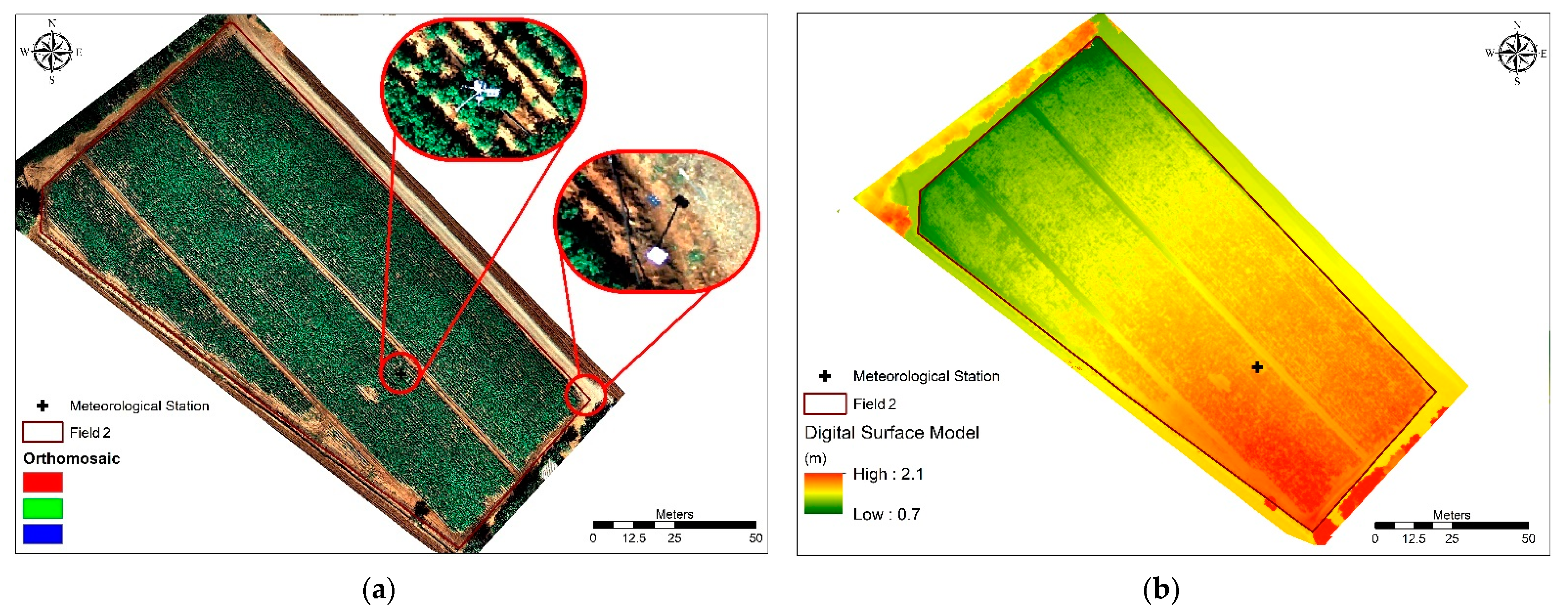
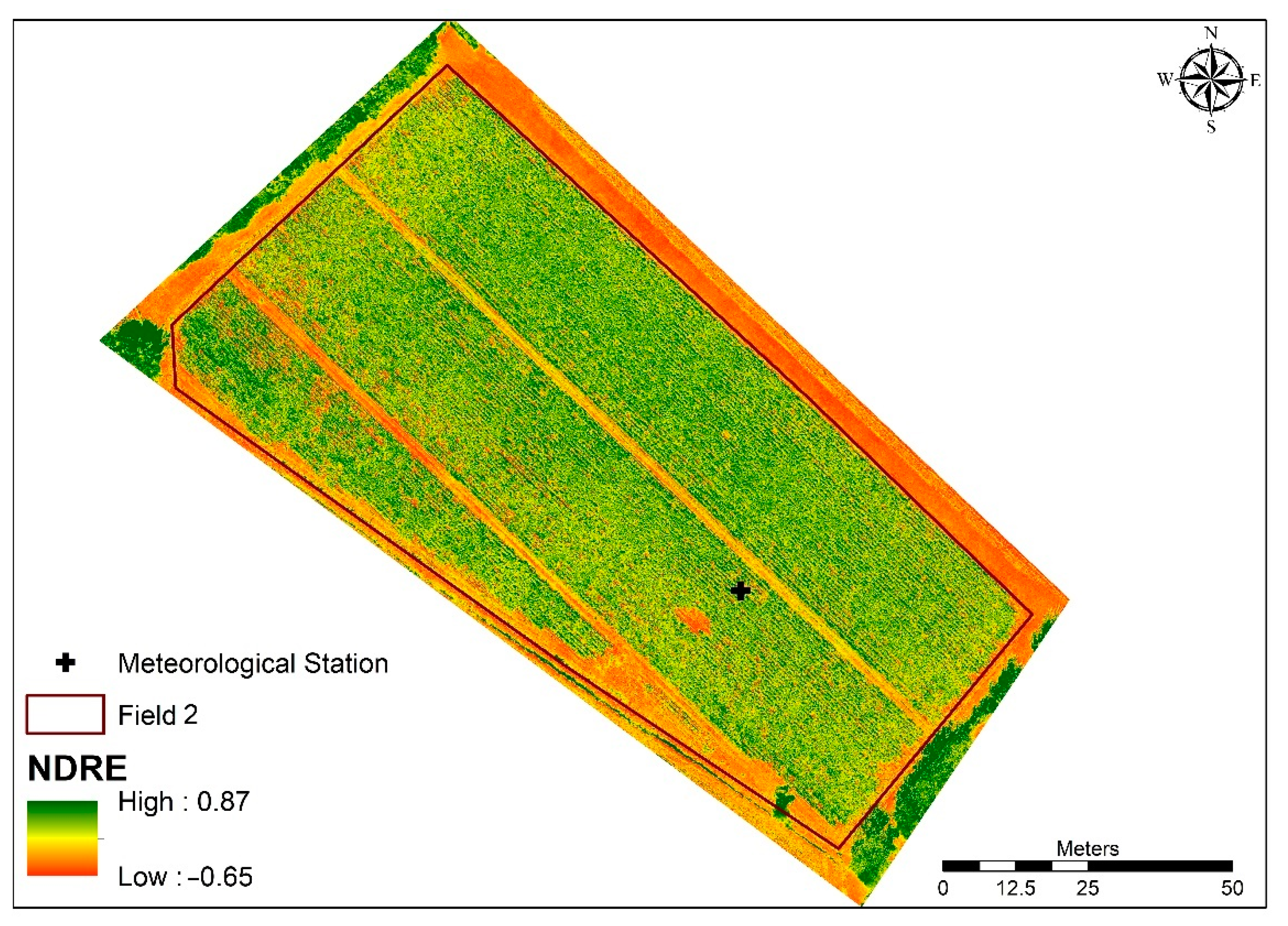
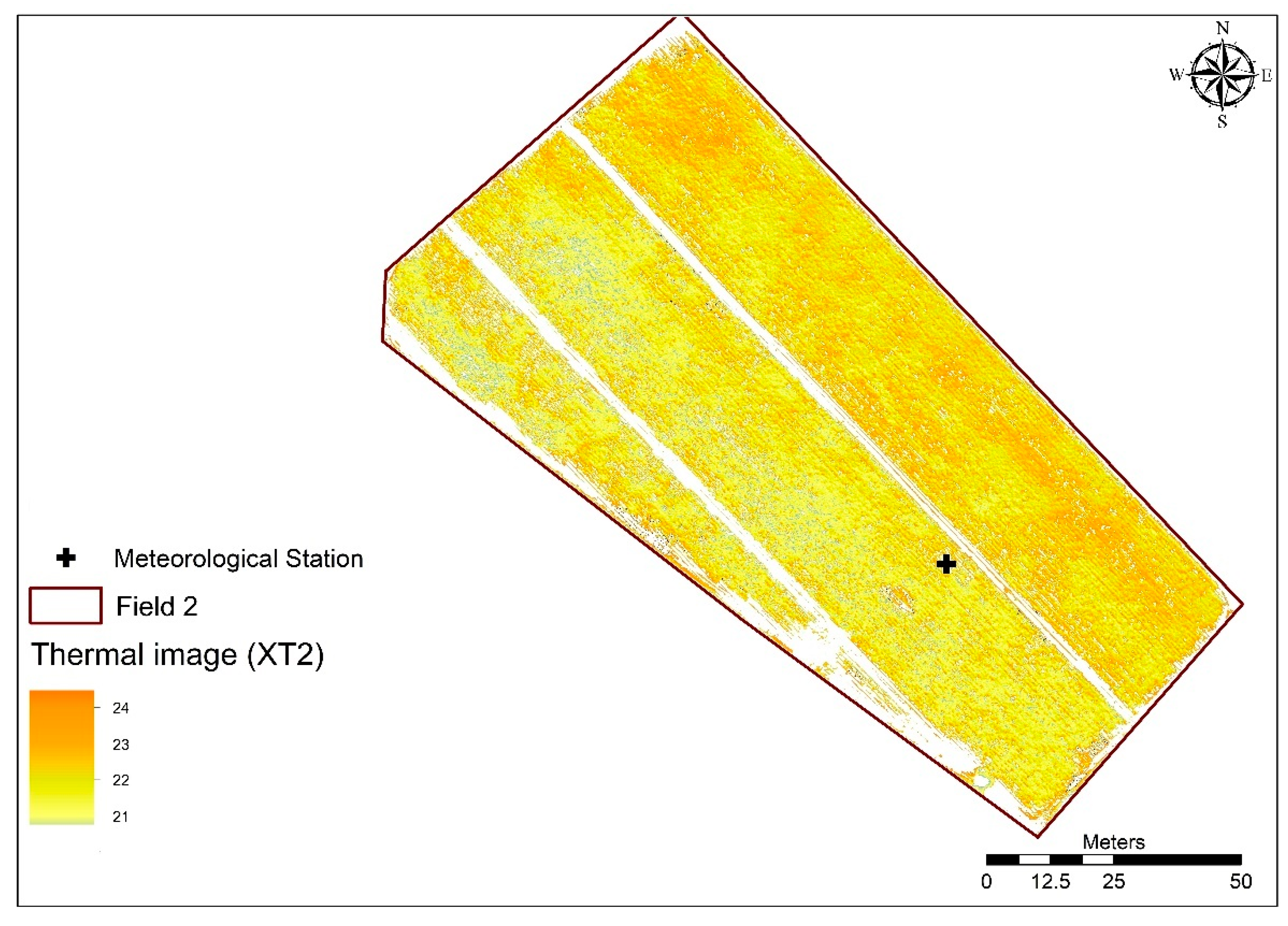
4.1. Photogrammetry—Multispectral and Thermal Imagery

The photogrammetric analysis provided very high-resolution information about the canopy conditions by creating the RGB true-color imagery of the field (Figure 13a), which revealed all the aspects of the canopy attributes and its surrounding area.

The DSM indicated a gentle inclination of the field, which was ideal for the appropriate drainage of the field and avoiding overlogging situations, where the elevation varied from 1.1 m at the south-southeastern part to 0.4 m at the north-northwestern part of the field (Figure 13b).

The result of the NDRE equation provided an image with continuum pixel values that ranged from −1 to 1, where negative values corresponded to non-vegetated surfaces, in this case, soil cover, while positive values corresponded to the vegetation reflectance (Figure 14). The values between 0.25 and 0.64 were related to healthy photosynthetic vegetation of potato canopy, while lower values, especially those <0.2, were related to stressed vegetation or bare soil. Values higher than 0.64 represented the dense tree cover in the northwestern and southeastern parts of the field. As it was mentioned before, the NDRE image was utilized to mask the soil cover from the co-registered TIR image (XT2) and the interpolation image derived from the IR sensor point values to produce the thermal products with pixels belonging only to sunlit leaves.

The thermal image (Figure 15) that was taken by the Zenmuse XT2 on the UAV was used to calculate the canopy temperature (T_c) of the experimental field. The image was classified (using custom classification), keeping only the pixels of the crop canopy area to separate and present the reliable foliage temperature values. The canopy temperatures (from the thermal image) ranged between approximately 21.2 and 24.3 °C (range of about 3 °C), which was very close to the station average IRT temperature (23.9 °C) and the average spatial IRT (21.8 °C), respectively. These measurements were taken during a day with clear sky conditions and relatively low temperatures. The crop was in the middle stage of growth (almost full canopy cover), where the soil and atmospheric conditions are presented in the following charts.

Although thermal RS has various potential advantages in crop monitoring, there are several practical difficulties in its use, including atmospheric attenuation and absorption, calibration, climatic conditions, crop growth stages, and complex soil and plant interaction that have to be adequately addressed.

The high-resolution multispectral and thermal imagery acquired using the UAV platform ideally enables the extraction and identification of crop conditions (vegetation vigor, spatial distribution, canopy cover, and bare ground gaps) and the temperature of the canopy. Furthermore, they demonstrate great capability for the recognition and monitoring of drought stress and were used in several different crops, such as potato, cotton, soybean, cotton, maize, vineyards, and orchards, over the last two decades [16,18,26,27,68,69,70,71]. Additionally, several studies showed that cloud cover and other haze or dew conditions can influence the quality of the thermal data obtained (due to lower contrast and poor radiometric resolution) [72,73,74]. Hence, these variables, along with relative humidity, altitude, and viewing angle, should be thoroughly examined while acquiring thermal data [71,73]. Moreover, the acquisition time during midday was demonstrated by several scientists that were the optimal time for thermal image acquisition [75].

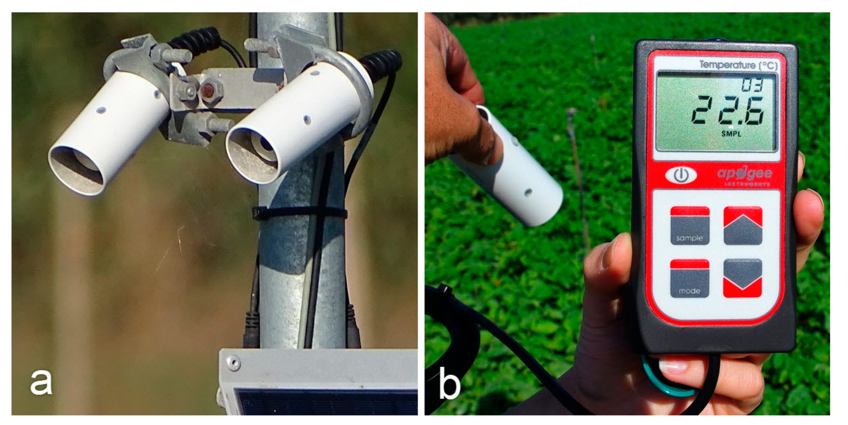
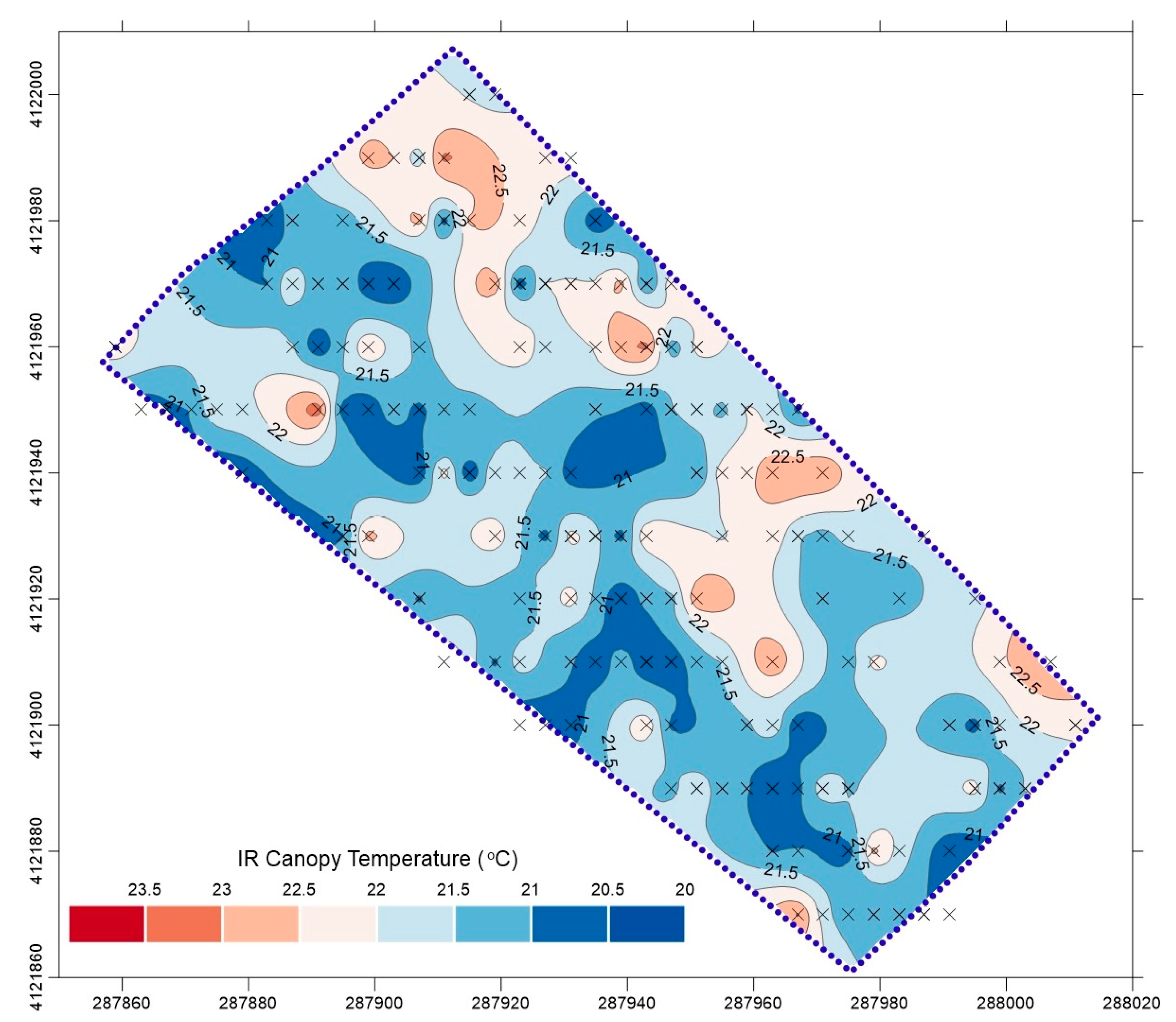
4.2. Direct Canopy IRT Measurements and Spatial CWSI Estimation

The first pilot flight with the UAV that brought the aMMS (aerial micrometeorological system) equipment took place on 25 October 2019 over field 2 during late potato cultivation. It was essentially the first comprehensive process for estimating the CWSI spatial mapping. In the same field, during the early cultivation of potatoes in May 2019, a previous estimation of CWSI calibration coefficients from specific days with ideal weather conditions was undertaken. We used all ground station data and parameters to determine the lower and upper baselines using theoretical and practical approaches. The day of the UAV flight was a clear sunny day with relatively low temperature levels, as the period was in the middle of autumn. The crop was in the middle stage of development. The UAV flight for the spatial measurements of the canopy temperature, air temperature, and relative humidity started at 12:14 p.m., which corresponded to the local solar time of the ground station (lat. 37.222194 N, long. 21.611806 E in degrees). The flight duration was 21 min, and 217 primary spatial measurements of infrared temperature from the crop canopy, air temperature, and relative humidity were collected from a height of 4 m above the ground (about 3.5 m from the top of the foliage). The flight was autonomous and scheduled following the standard flight plan described in Section 3.3.1 (Figure 8). The speed of the quadcopter was 1 m/s, and the excitation of the sensors for measurement was every 6 s (measurement every 6 m along the flight line). All microclimatic data obtained from the ground station (GMMS) above the crop, as well as the mean spatial values (N = 217) from the sensors of the aerial micrometeorological system, are shown in

Table 1. Ten-minute average climatic data from the ground micrometeorological station (GMMS) from field 2 and the averages values from 217 measurements of the air temperature, canopy infrared temperature, and relative humidity from the aerial micrometeorological system (AMMS).

Solar Time	Tair	IRT	RH	Wind Direction	Wind Speed	Solar Radiation	Net Radiation
	(°C)		(%)	(°)	(ms−1)	(Wm−2)
12:15	23.9	23.4	66.6	314	1.6	675	399
12:25	24.0	24.0	64.1	320	1.5	667	394
12:35	24.1	24.2	62.2	320	1.2	665	393
GMMS *	24.0	23.9	64.3	318	1.4	669	395
AMMS *	24.3	21.8	56.0

* Mean values of measurements.

.

Moreover,

Table 2. Soil water moisture (vol%) for the depth of 60 cm of the soil profile in the potato field.

	Volumetric Soil Water Content (%) of the Soil Layer (in cm)						Soil Heat Flux
Time	0–10	10–20	20–30	30–40	40–50	50–60	(Wm−2)
12:30 p.m.	4.7	8.6	25.4	39.2	39.1	21.3	23.7
12:40 p.m.	4.7	8.6	25.3	39.2	39.1	21.3	23.5
12:50 p.m.	4.7	8.5	25.2	39.2	39.1	21.3	23.2
Average	4.7	8.6	25.3	39.2	39.1	21.3	23.5

presents the moisture conditions in the six layers (from 0–60 cm with 10 cm intervals), and the soil heat flux density at a depth of 8 cm. As shown in Figure 16, the surface layer (0–10 cm) had lost 67% of its moisture from the total height of the available water between two irrigation events. Usually, the irrigation frequency for this period was every 3–4 days, as shown in Figure 16 for the last three irrigation events (16, 20, and 23 October 19).

Figure 17 presents the isothermal lines from a spatial-observation-derived analysis (N = 217) using the geostatistical gridding Kriging method, which produces maps from atypical, spaced data.

The method is very flexible and produces an accurate data grid by a smoothing interpolator depending on the user-specified parameters. The spacing nodes grid size used 86 rows × 100 columns (total nodes: 8600). Some univariate grid statistics for the canopy IR temperature for the grid data (in °C) were min: 21.603, max: 22.133, mean: 21.886, root mean square: 21.8869, standard deviation: 0.1486, average abs. deviation: 0.1252, and relative mean diff.: 0.0078.

The exact area (enclosed area by the boundary line) of field 2 was 9940.3 m². Each observation was taken from about 4 m above the crop and corresponded to the mean value of the infrared temperature of the circular surface of the cone base radius (target) of about 3 m (Figure 8).

The evaluation of the CWSI index during the clear sky and dry hours of the day offered a real and more direct method to determine the ideal time for irrigation, as it effectively found and normalized the short-term microclimatic changes of the environment in which the crop grew up and responded reliably to maintaining the optimal water content of the soil porosity into the rhizosphere zone. This significantly improved the irrigation efficiency and water-saving at all stages of plant growth. The spatial estimates of the CWSI are shown in Figure 18.

The calibration resulting from the spring potato cultivation (non-stressed lower baseline: T_c − T_a = −1.74 × VPD − 1.23, stressed upper baseline T_c − T_a = 2.32 °C) was used in the first pilot approach of the spatial CWSI in the autumn potato cultivation. The high relative humidity that prevailed during the calibration season, in combination with the low temperatures, gave a limited range of vapor pressure deficit of the atmosphere (VPD), leading to a high slope of the lower non-stressed baseline bottom line with a relatively high dispersion of the observed measurements (r² = 0.613). However, this calibration provided satisfactory values for the spatial CWSI estimates in conjunction with the actual water loss from the ground profile just before the next irrigation (Figure 16 and Table 2).

5. Conclusions

The integration of new, improved methods and tools in modern agriculture, combined with the limitations of the water availability for irrigation, pushes research into new and smart approaches. A major advantage in this context is that, nowadays, it is both feasible and affordable to use proven and reliable methods that required expensive instruments and high installation costs in the past. Furthermore, in agricultural production, the involvement of irrigation water is crucial in maintaining the quality and conservation of it as a natural resource.

Nowadays, the use of UAVs in agriculture is universal. The continuous evolution of UAV technology with lighter materials and the evolution of battery technology allows for long flight periods with heavier equipment loads. However, spatial data from crops are mostly acquired only through multispectral and thermal cameras to date.

Taking advantage of the UAV evolution, GreenWaterDrone (GWD) proposes an innovative system, integrating aerial measurements of canopy temperatures for the near-real-time calculation of crop irrigation needs (crop water stress detection) and dynamic crop surveillance, achieving measurements with high temporal and spatial resolution, while at the same time, minimizing the intervention in crop activities and system maintenance costs. The GWD solution is especially suited for relatively small fields with increased crop diversity that cannot be efficiently addressed by satellite remote sensing. An onboard aerial micrometeorological system (AMMS) allows for calculating the known CWSI (crop water stress index) in spatial estimation for many crops in the area. Using the thermal images in parallel with spatial measurements by the infrared radiometers is an advantage that allows us to compare and calibrate the methodology at an accurate level. Furthermore, it must be noted that the estimation of the CWSI at the implementation level is achieved by the spatial estimates of the infrared thermometers from UAVs (AMMS). Moreover, it must be mentioned that the multispectral and photogrammetric cameras significantly assist the results by providing information concerning the canopy cover and field conditions useful for crop surveillance.

In this work, we present the GWD methodology, along with the equipment specifications used. All processes at all steps of applying the methodology on a pilot potato field are described, and preliminary results from the application are presented. From the pilot study, the functionality of the proposed system (GWD) was certified (accuracy of the UAV path and flight altitude, reliability of the aerial data acquisition system, communication stability between UAVs and ground base). Our findings indicated that the canopy temperatures derived from the ground meteorological station (GMMS), the AMMS, and the portable IRT radiometers produced a suitable thermal image from the surface of the crop. However, it should be noted that the scheduled flight took place in the middle of the autumn season when the crop evapotranspiration rate was very low (ET_c was 2.7 mm/d and the soil moisture profile remained almost unchanged).

The project subsystems can be useful for supporting applications that are significant for irrigation water management and programming, such as irrigation alerting and scheduling, crop surveillance, and irrigation water management. However, more efforts are necessary to make these technologies more user-friendly and available for all end users, covering different advantages for a precise crop water stress evaluation. Still, the stakeholders, farmers, and industry responded positively to this effort’s augmented interest. Furthermore, similar pilot campaigns need to be conducted in other regions on different crops to enhance the applicability of the GWD system. There is ongoing work by the authors to collect data for calibrating the methodology for other crops.

References

1. Bin Abdullah, K. Use of water and land for food security and environmental sustainability. Irrig. Drain. 2006, 55, 219–222. [Google Scholar] [CrossRef]
2. Mulla, D.; Miao, Y. Precision Farming; CRC Press: Boca Raton, FL, USA, 2015; pp. 161–178. [Google Scholar]
3. Yang, Y.; Shang, S.; Jiang, L. Remote sensing temporal and spatial patterns of evapotranspiration and the responses to water management in a large irrigation district of North China. Agric. For. Meteorol. 2012, 164, 112–122. [Google Scholar] [CrossRef]
4. Peña-Arancibia, J.L.; Mainuddin, M.; Kirby, J.M.; Chiew, F.H.S.; McVicar, T.R.; Vaze, J. Assessing irrigated agriculture’s surface water and groundwater consumption by combining satellite remote sensing and hydrologic modelling. Sci. Total Environ. 2016, 542, 372–382. [Google Scholar] [CrossRef] [PubMed]
5. Vecchio, Y.; De Rosa, M.; Adinolfi, F.; Bartoli, L.; Masi, M. Adoption of precision farming tools: A context-related analysis. Land Use Policy 2020, 94, 104481. [Google Scholar] [CrossRef]
6. Tsouros, D.C.; Bibi, S.; Sarigiannidis, P.G. A review on UAV-based applications for precision agriculture. Information 2019, 10, 349. [Google Scholar] [CrossRef] [Green Version]
7. Alexandris, S.; Proutsos, N. How significant is the effect of the surface characteristics on the Reference Evapotranspiration estimates? Agric. Water Manag. 2020, 237, 106181. [Google Scholar] [CrossRef]
8. Egea, G.; Padilla-Díaz, C.M.; Martinez-Guanter, J.; Fernández, J.E.; Pérez-Ruiz, M. Assessing a crop water stress index derived from aerial thermal imaging and infrared thermometry in super-high density olive orchards. Agric. Water Manag. 2017, 187, 210–221. [Google Scholar] [CrossRef] [Green Version]
9. Xie, Y.; Sha, Z.; Yu, M. Remote sensing imagery in vegetation mapping: A review. J. Plant. Ecol. 2008, 1, 9–23. [Google Scholar] [CrossRef]
10. Kavvadias, A.; Psomiadis, E.; Chanioti, M.; Gala, E.; Michas, S. Precision agriculture—Comparison and evaluation of innovative very high resolution (UAV) and LandSat data. In Proceedings of the 7th International Conference on Information and Communication Technologies in Agriculture, Food and Environment (HAICTA 2015), Kavala, Greece, 17–20 September 2015; Volume 1498. [Google Scholar]
11. Kavvadias, A.; Psomiadis, E.; Chanioti, M.; Tsitouras, A.; Toulios, L.; Dercas, N. Unmanned Aerial Vehicle (UAV) data analysis for fertilization dose assessment. In Proceedings of the SPIE—Remote Sensing for Agriculture, Ecosystems, and Hydrology XIX, Warsaw, Poland, 11–14 September 2017; Volume 10421. [Google Scholar]
12. Gago, J.; Douthe, C.; Coopman, R.E.; Gallego, P.P.; Ribas-Carbo, M.; Flexas, J.; Escalona, J.; Medrano, H. UAVs challenge to assess water stress for sustainable agriculture. Agric. Water Manag. 2015, 153, 9–19. [Google Scholar] [CrossRef]
13. Jones, H.; Sirault, X. Scaling of Thermal Images at Different Spatial Resolution: The Mixed Pixel Problem. Agronomy 2014, 4, 380–396. [Google Scholar] [CrossRef] [Green Version]
14. Nahry, A.H.E.; Ali, R.R.; Baroudy, A.A.E. An approach for precision farming under pivot irrigation system using remote sensing and GIS techniques. Agric. Water Manag. 2011, 98, 517–531. [Google Scholar] [CrossRef]
15. Anderson, K.; Gaston, K.J. Lightweight unmanned aerial vehicles will revolutionize spatial ecology. Front. Ecol. Environ. 2013, 11, 138–146. [Google Scholar] [CrossRef] [Green Version]
16. Zhang, L.; Niu, Y.; Zhang, H.; Han, W.; Li, G.; Tang, J.; Peng, X. Maize Canopy Temperature Extracted From UAV Thermal and RGB Imagery and Its Application in Water Stress Monitoring. Front. Plant. Sci. 2019, 10, 1270. [Google Scholar] [CrossRef]
17. Zhang, C.; Kovacs, J.M. The application of small unmanned aerial systems for precision agriculture: A review. Precis. Agric. 2012, 13, 693–712. [Google Scholar] [CrossRef]
18. Rud, R.; Cohen, Y.; Alchanatis, V.; Levi, A.; Brikman, R.; Shenderey, C.; Heuer, B.; Markovitch, T.; Dar, Z.; Rosen, C.; et al. Crop water stress index derived from multi-year ground and aerial thermal images as an indicator of potato water status. Precis. Agric. 2014, 15, 273–289. [Google Scholar] [CrossRef]
19. Cucho-Padin, G.; Rinza, J.; Ninanya, J.; Loayza, H.; Quiroz, R.; Ramírez, D.A. Development of an Open-Source Thermal Image Processing Software for Improving Irrigation Management in Potato Crops (Solanum tuberosum L.). Sensors 2020, 20, 472. [Google Scholar] [CrossRef] [PubMed] [Green Version]
20. Veysi, S.; Naseri, A.A.; Hamzeh, S.; Bartholomeus, H. A satellite based crop water stress index for irrigation scheduling in sugarcane fields. Agric. Water Manag. 2017, 189, 70–86. [Google Scholar] [CrossRef]
21. Lebourgeois, V.; Labbé, S.; Jacob, F.; Bégué, A. Atmospheric corrections of low altitude thermal infrared airborne images acquired over a tropical cropped area. In Proceedings of the International Geoscience and Remote Sensing Symposium (IGARSS), Boston, MA, USA, 7–11 July 2008; Institute of Electrical and Electronics Engineers Inc.: Piscataway, NJ, USA, 2008; Volume 3, pp. 672–675. [Google Scholar]
22. da Silva, B.B.; Ferreira, J.A.; Rammana, T.V.; Rodríguez, V.P. Crop Water Stress Index and Water-Use Efficiency for Melon (Cucumis melo L.) on Different Irrigation Regimes. Agric. J. 2007, 2, 31–37. [Google Scholar]
23. Sepulcre-Cantó, G.; Zarco-Tejada, P.J.; Jiménez-Muñoz, J.C.; Sobrino, J.A.; De Miguel, E.; Villalobos, F.J. Detection of water stress in an olive orchard with thermal remote sensing imagery. Agric. For. Meteorol. 2006, 136, 31–44. [Google Scholar] [CrossRef]
24. Gutiérrez, S.; Diago, M.P.; Fernández-Novales, J.; Tardaguila, J. Vineyard water status assessment using on-the-go thermal imaging and machine learning. PLoS ONE 2018, 13, e0192037. [Google Scholar] [CrossRef]
25. Baluja, J.; Diago, M.P.; Balda, P.; Zorer, R.; Meggio, F.; Morales, F.; Tardaguila, J. Assessment of vineyard water status variability by thermal and multispectral imagery using an unmanned aerial vehicle (UAV). Irrig. Sci. 2012, 30, 511–522. [Google Scholar] [CrossRef]
26. Moller, M.; Alchanatis, V.; Cohen, Y.; Meron, M.; Tsipris, J.; Naor, A.; Ostrovsky, V.; Sprintsin, M.; Cohen, S. Use of thermal and visible imagery for estimating crop water status of irrigated grapevine. J. Exp. Bot. 2006, 58, 827–838. [Google Scholar] [CrossRef] [Green Version]
27. Zhang, L.; Zhang, H.; Niu, Y.; Han, W. Mapping Maize Water Stress Based on UAV Multispectral Remote Sensing. Remote Sens. 2019, 11, 605. [Google Scholar] [CrossRef] [Green Version]
28. Yang, W.; Li, C.; Yang, H.; Yang, G.; Feng, H.; Han, L.; Niu, Q.; Han, D. Monitoring of canopy temperature of maize based on UAV thermal infrared imagery and digital imagery. Nongye Gongcheng Xuebao/Trans. Chin. Soc. Agric. Eng. 2018, 34, 68–75. [Google Scholar] [CrossRef]
29. Gonzalez-Dugo, V.; Zarco-Tejada, P.; Nicolás, E.; Nortes, P.A.; Alarcón, J.J.; Intrigliolo, D.S.; Fereres, E. Using high resolution UAV thermal imagery to assess the variability in the water status of five fruit tree species within a commercial orchard. Precis. Agric. 2013, 14, 660–678. [Google Scholar] [CrossRef]
30. Bellvert, J.; Zarco-Tejada, P.J.; Girona, J.; Fereres, E. Mapping crop water stress index in a “Pinot-noir” vineyard: Comparing ground measurements with thermal remote sensing imagery from an unmanned aerial vehicle. Precis. Agric. 2014, 15, 361–376. [Google Scholar] [CrossRef]
31. Berni, J.A.J.; Zarco-Tejada, P.J.; Suárez, L.; Fereres, E. Thermal and narrowband multispectral remote sensing for vegetation monitoring from an unmanned aerial vehicle. IEEE Trans. Geosci. Remote Sens. 2009, 47, 722–738. [Google Scholar] [CrossRef] [Green Version]
32. Matese, A.; Baraldi, R.; Berton, A.; Cesaraccio, C.; Di Gennaro, S.; Duce, P.; Facini, O.; Mameli, M.; Piga, A.; Zaldei, A. Estimation of Water Stress in Grapevines Using Proximal and Remote Sensing Methods. Remote Sens. 2018, 10, 114. [Google Scholar] [CrossRef] [Green Version]
33. Santesteban, L.G.; Di Gennaro, S.F.; Herrero-Langreo, A.; Miranda, C.; Royo, J.B.; Matese, A. High-resolution UAV-based thermal imaging to estimate the instantaneous and seasonal variability of plant water status within a vineyard. Agric. Water Manag. 2017, 183, 49–59. [Google Scholar] [CrossRef]
34. Jackson, R.D.; Idso, S.B.; Reginato, R.J.; Pinter, P.J. Canopy temperature as a crop water stress indicator. Water Resour. Res. 1981, 17, 1133–1138. [Google Scholar] [CrossRef]
35. Idso, S.B.; Jackson, R.D.; Pinter, P.J.; Reginato, R.J.; Hatfield, J.L. Normalizing the stress-degree-day parameter for environmental variability. Agric. Meteorol. 1981, 24, 45–55. [Google Scholar] [CrossRef]
36. Jackson, R.D.; Kustas, W.P.; Choudhury, B.J. A reexamination of the crop water stress index. Irrig. Sci. 1988, 9, 309–317. [Google Scholar] [CrossRef]
37. Awais, M.; Li, W.; Cheema, M.J.M.; Hussain, S.; AlGarni, T.S.; Liu, C.; Ali, A. Remotely sensed identification of canopy characteristics using UAV-based imagery under unstable environmental conditions. Environ. Technol. Innov. 2021, 22, 101465. [Google Scholar] [CrossRef]
38. Mwinuka, P.R.; Mbilinyi, B.P.; Mbungu, W.B.; Mourice, S.K.; Mahoo, H.F.; Schmitter, P. The feasibility of hand-held thermal and UAV-based multispectral imaging for canopy water status assessment and yield prediction of irrigated African eggplant (Solanum aethopicum L.). Agric. Water Manag. 2021, 245, 106584. [Google Scholar] [CrossRef]
39. Shao, G.; Han, W.; Zhang, H.; Liu, S.; Wang, Y.; Zhang, L.; Cui, X. Mapping maize crop coefficient Kc using random forest algorithm based on leaf area index and UAV-based multispectral vegetation indices. Agric. Water Manag. 2021, 252, 106906. [Google Scholar] [CrossRef]
40. Zhou, Z.; Majeed, Y.; Diverres Naranjo, G.; Gambacorta, E.M.T. Assessment for crop water stress with infrared thermal imagery in precision agriculture: A review and future prospects for deep learning applications. Comput. Electron. Agric. 2021, 182, 106019. [Google Scholar] [CrossRef]
41. de Castro, A.I.; Shi, Y.; Maja, J.M.; Peña, J.M. UAVs for Vegetation Monitoring: Overview and Recent Scientific Contributions. Remote Sens. 2021, 13, 2139. [Google Scholar] [CrossRef]
42. Han, Y.; Tarakey, B.A.; Hong, S.-J.; Kim, S.-Y.; Kim, E.; Lee, C.-H.; Kim, G. Calibration and Image Processing of Aerial Thermal Image for UAV Application in Crop Water Stress Estimation. J. Sens. 2021, 2021, 1–14. [Google Scholar] [CrossRef]
43. Zhang, L.; Han, W.; Niu, Y.; Chávez, J.L.; Shao, G.; Zhang, H. Evaluating the sensitivity of water stressed maize chlorophyll and structure based on UAV derived vegetation indices. Comput. Electron. Agric. 2021, 185, 106174. [Google Scholar] [CrossRef]
44. Irmak, S.; Haman, D.Z.; Bastug, R. Determination of Crop Water Stress Index for Irrigation Timing and Yield Estimation of Corn. Agron. J. 2000, 92, 1221–1227. [Google Scholar] [CrossRef]
45. Thom, A.S. Momentum, mass and heat exchange of vegetation. Q. J. R. Meteorol. Soc. 1972, 98, 124–134. [Google Scholar] [CrossRef]
46. Monteith, J.; Unsworth, M. Principles of Environmental Physics: Plants, Animals, and the Atmosphere; Academic Press: Cambridge, MA, USA, 2013. [Google Scholar]
47. Brutsaert, W. Evaporation into the Atmosphere: Theory, History and Applications; Springer: Berlin/Heidelberg, Germany, 2013. [Google Scholar]
48. Clothier, B.E.; Clawson, K.L.; Pinter, P.J.; Moran, M.S.; Reginato, R.J.; Jackson, R.D. Estimation of soil heat flux from net radiation during the growth of alfalfa. Agric. For. Meteorol. 1986, 37, 319–329. [Google Scholar] [CrossRef]
49. Thom, A.S.; Oliver, H.R. On Penman’s equation for estimating regional evaporation. Q. J. R. Meteorol. Soc. 1977, 103, 345–357. [Google Scholar] [CrossRef]
50. Thornthwaite, C.W. An Approach toward a Rational Classification of Climate. Geogr. Rev. 1948, 38, 55. [Google Scholar] [CrossRef]
51. Tsiros, I.X.; Nastos, P.; Proutsos, N.D.; Tsaousidis, A. Variability of the aridity index and related drought parameters in Greece using climatological data over the last century (1900–1997). Atmos. Res. 2020, 240, 104914. [Google Scholar] [CrossRef]
52. McEvoy, J.F.; Hall, G.P.; Mcdonald, P.G. Evaluation of unmanned aerial vehicle shape, flight path and camera type for waterfowl surveys: Disturbance effects and species recognition. PeerJ 2016, 4, e1831. [Google Scholar] [CrossRef] [PubMed] [Green Version]
53. Mouazen, A.M.; Alexandridis, T.; Buddenbaum, H.; Cohen, Y.; Moshou, D.; Mulla, D.; Nawar, S.; Sudduth, K.A. Monitoring. In Agricultural Internet of Things and Decision Support for Precision Smart Farming; Elsevier Inc.: Amsterdam, The Netherlands, 2020; pp. 35–138. ISBN 9780128183731. [Google Scholar]
54. Verhoeven, G.; Doneus, M.; Briese, C.; Vermeulen, F. Mapping by matching: A computer vision-based approach to fast and accurate georeferencing of archaeological aerial photographs. J. Archaeol. Sci. 2012, 39, 2060–2070. [Google Scholar] [CrossRef]
55. Alexiou, S.; Deligiannakis, G.; Pallikarakis, A.; Papanikolaou, I.; Psomiadis, E.; Reicherter, K. Comparing High Accuracy t-LiDAR and UAV-SfM Derived Point Clouds for Geomorphological Change Detection. ISPRS Int. J. Geo-Inf. 2021, 10, 367. [Google Scholar] [CrossRef]
56. Kung, O.; Strecha, C.; Beyeler, A.; Zufferey, J.-C.; Floreano, D.; Fua, P.; Gervaix, F. The accuracy of automatic photogrammetric techniques on ultra-light UAV imagery. In Proceedings of the UAV-g 2011—Unmanned Aerial Vehicle in Geomatics, Zürich, Switzerland, 14–16 September 2011. [Google Scholar]
57. Darra, N.; Psomiadis, E.; Kasimati, A.; Anastasiou, A.; Anastasiou, E.; Fountas, S. Remote and Proximal Sensing-Derived Spectral Indices and Biophysical Variables for Spatial Variation Determination in Vineyards. Agronomy 2021, 11, 741. [Google Scholar] [CrossRef]
58. Andriolo, U.; Gonçalves, G.; Bessa, F.; Sobral, P. Mapping marine litter on coastal dunes with unmanned aerial systems: A showcase on the Atlantic Coast. Sci. Total Environ. 2020, 736, 139632. [Google Scholar] [CrossRef] [PubMed]
59. Rud, R.; Shoshany, M.; Alchanatis, V. Spatial-spectral processing strategies for detection of salinity effects in cauliflower, aubergine and kohlrabi. Biosyst. Eng. 2013, 114, 384–396. [Google Scholar] [CrossRef]
60. Melis, M.T.; Da Pelo, S.; Erbì, I.; Loche, M.; Deiana, G.; Demurtas, V.; Meloni, M.A.; Dessì, F.; Funedda, A.; Scaioni, M.; et al. Thermal remote sensing from UAVs: A review on methods in coastal cliffs prone to landslides. Remote Sens. 2020, 12, 1971. [Google Scholar] [CrossRef]
61. Processing Thermal Images—Support. Available online: https://support.pix4d.com/hc/en-us/articles/360000173463-Processing-thermal-images (accessed on 15 June 2021).
62. López, A.; Jurado, J.M.; Ogayar, C.J.; Feito, F.R. A framework for registering UAV-based imagery for crop-tracking in Precision Agriculture. Int. J. Appl. Earth Obs. Geoinf. 2021, 97, 102274. [Google Scholar] [CrossRef]
63. Bellvert, J.; Zarco-Tejada, P.J.; Marsal, J.; Girona, J.; González-Dugo, V.; Fereres, E. Vineyard irrigation scheduling based on airborne thermal imagery and water potential thresholds. Aust. J. Grape Wine Res. 2016, 22, 307–315. [Google Scholar] [CrossRef] [Green Version]
64. García-Tejero, I.F.; Costa, J.M.; Egipto, R.; Durán-Zuazo, V.H.; Lima, R.S.N.; Lopes, C.M.; Chaves, M.M. Thermal data to monitor crop-water status in irrigated Mediterranean viticulture. Agric. Water Manag. 2016, 176, 80–90. [Google Scholar] [CrossRef]
65. Tang, Z.; Parajuli, A.; Chen, C.J.; Hu, Y.; Revolinski, S.; Medina, C.A.; Lin, S.; Zhang, Z.; Yu, L.X. Validation of UAV-based alfalfa biomass predictability using photogrammetry with fully automatic plot segmentation. Sci. Rep. 2021, 11, 3336. [Google Scholar] [CrossRef] [PubMed]
66. Bian, J.; Zhang, Z.; Chen, J.; Chen, H.; Cui, C.; Li, X.; Chen, S.; Fu, Q. Simplified Evaluation of Cotton Water Stress Using High Resolution Unmanned Aerial Vehicle Thermal Imagery. Remote Sens. 2019, 11, 267. [Google Scholar] [CrossRef] [Green Version]
67. Sagan, V.; Maimaitijiang, M.; Sidike, P.; Eblimit, K.; Peterson, K.; Hartling, S.; Esposito, F.; Khanal, K.; Newcomb, M.; Pauli, D.; et al. UAV-Based High Resolution Thermal Imaging for Vegetation Monitoring, and Plant Phenotyping Using ICI 8640 P, FLIR Vue Pro R 640, and thermoMap Cameras. Remote Sens. 2019, 11, 330. [Google Scholar] [CrossRef] [Green Version]
68. Vamvakoulas, C.; Argyrokastritis, I.; Papastylianou, P.; Papatheohari, Y.; Alexandris, S. Crop water stress index relationship with soybean seed, protein and oil yield under varying irrigation regimes in a Mediterranean environment. Isr. J. Plant. Sci. 2020, 67, 1–13. [Google Scholar] [CrossRef]
69. Cohen, Y.; Alchanatis, V.; Sela, E.; Saranga, Y.; Cohen, S.; Meron, M.; Bosak, A.; Tsipris, J.; Ostrovsky, V.; Orolov, V.; et al. Crop water status estimation using thermography: Multi-year model development using ground-based thermal images. Precis. Agric. 2015, 16, 311–329. [Google Scholar] [CrossRef]
70. Cohen, Y.; Alchanatis, V.; Saranga, Y.; Rosenberg, O.; Sela, E.; Bosak, A. Mapping water status based on aerial thermal imagery: Comparison of methodologies for upscaling from a single leaf to commercial fields. Precis. Agric. 2017, 18, 801–822. [Google Scholar] [CrossRef]
71. Berni, J.A.J.; Zarco-Tejada, P.J.; Sepulcre-Cantó, G.; Fereres, E.; Villalobos, F. Mapping canopy conductance and CWSI in olive orchards using high resolution thermal remote sensing imagery. Remote Sens. Environ. 2009, 113, 2380–2388. [Google Scholar] [CrossRef]
72. Thomson, S.J.; Ouellet-Plamondon, C.M.; DeFauw, S.L.; Huang, Y.; Fisher, D.K.; English, P.J. Potential and Challenges in Use of Thermal Imaging for Humid Region Irrigation System Management. J. Agric. Sci. 2012, 4, p103. [Google Scholar] [CrossRef]
73. Khanal, S.; Fulton, J.; Shearer, S. An overview of current and potential applications of thermal remote sensing in precision agriculture. Comput. Electron. Agric. 2017, 139, 22–32. [Google Scholar] [CrossRef]
74. Fuchs, M.; Kanemasu, E.T.; Kerr, J.P.; Tanner, C.B. Effect of Viewing Angle on Canopy Temperature Measurements with Infrared Thermometers. Agron. J. 1967, 59, 494–496. [Google Scholar] [CrossRef]
75. Alchanatis, V.; Cohen, Y.; Cohen, S.; Moller, M.; Sprinstin, M.; Meron, M.; Tsipris, J.; Saranga, Y.; Sela, E. Evaluation of different approaches for estimating and mapping crop water status in cotton with thermal imaging. Precis. Agric. 2010, 11, 27–41. [Google Scholar] [CrossRef]
Figure 1. A schematic representation of the CWSI, which equals the relative distance of the measurement between the lower and the upper baselines.
Hydrology 08 00131 g001
Figure 2. The concise physical architecture of the system with the basic physical entities, implementing the respective groups of functional entities and their placement in the above subsystems, as well as the relevant interfaces between entities and subsystems.
Hydrology 08 00131 g002
Figure 3. Location of the GWD project’s experimental fields in Trifilia.
Hydrology 08 00131 g003
Figure 4. (a) Experimental field 2 with the potato cultivation; (b) categorization of the soils of the three experimental fields at depths of 0–20, 20–40, and 40–60 cm in the soil triangle. The soil texture classification according to the USDA (U.S. Department of Agriculture).
Hydrology 08 00131 g004
Figure 5. Three stations were installed in the middle of the experimental fields: (a) the first station in field 1, with early watermelon cultivation with a plastic cover for protection against the spring frost; (b) the second station in field 2 with the cultivation of spring potato in the middle growing stage; (c) the third station installed in field 3 with young tomato plants.
Hydrology 08 00131 g005
Figure 6. Soil water content isolines (%) in the irrigated spring potato crop (field 2) for 10 May–9 July 2019 (DOY: 130–181).
Hydrology 08 00131 g006
Figure 7. (a) Watertight box (data logger Stylitis-12 inside); (b) temperature and relative humidity (thermo-hygrometer) sensor in the radiation shield; (c) infrared sensor and the mounting base; (d) GPS sensor.
Hydrology 08 00131 g007
Figure 8. Graphic illustration of the measurement process with an infrared radiometer adapted to a UAV over dense cultivation foliage under a clear sky. The flight height depends on the sensor type and the characteristics of the crop. For a specific IRT sensor, the visible surface area is a function of height. For the sensor SI-111 that was placed vertically to the foliage with a height of flight h = 4 m, the surface area was E = 8.2 m2, and the diameter of the circular surface was about 3.2 m.
Hydrology 08 00131 g008
Figure 9. (a) The fixed-wing Q100 Datahawk; (b) the multispectral Sentera camera; (c) the thermal infrared camera Zenmuse XT2.
Hydrology 08 00131 g009
Figure 10. The field measurements that were taken using the IR sensors on (a) the meteorological station and (b) a portable device.
Hydrology 08 00131 g010
Figure 11. (a) The RTK GNSS that was used for the collection of the GCPs; (b) the rectangular aluminum plates that were used as ground control points on the field.
Hydrology 08 00131 g011
Figure 12. Hourly values for the date 25/10/2019 for the (a) global solar radiation Rs, net radiation Rnet, photosynthetically active radiation PAR, and soil heat flux SHF; (b) air and canopy temperatures; (c) vapor pressure deficit VPD, wind speed WS, crop evapotranspiration; (d) soil moisture profile for six depths measured in the potato field.
Hydrology 08 00131 g012
Figure 13. (a) The very high-resolution true color orthomosaic and (b) the very high-resolution digital surface model of field 2.
Hydrology 08 00131 g013
Figure 14. The red-edge normalized difference vegetation index of field 2, which was calculated using the multispectral camera data.
Hydrology 08 00131 g014
Figure 15. Thermal image acquired by the Zenmuse XT2 camera showing only the crop vegetation’s temperature values by masking all the non-vegetation pixels.
Hydrology 08 00131 g015
Figure 16. The fluctuation of the soil moisture in the surface layer of the soil (0–10 cm) after three consecutive irrigations.
Hydrology 08 00131 g016
Figure 17. The temperature values that were derived from the IR sensor measurements.
Hydrology 08 00131 g017
Figure 18. Spatial estimates (isolines of CWSI) from the first pilot flight with AMMS.
Hydrology 08 00131 g018