Abstract
We describe modified sampling and analysis methods to quantify nutrient atmospheric deposition (AD) and estimate Utah Lake nutrient loading. We address criticisms of previous published collection methods, specifically collection table height, screened buckets, and assumptions of AD spatial patterns. We generally follow National Atmospheric Deposition Program (NADP) recommendations but deviate to measure lake AD, which includes deposition from both local and long-range sources. The NADP guidelines are designed to eliminate local contributions to the extent possible, while lake AD loads should include local contributions. We collected side-by-side data with tables at 1 m (previous results) and 2 m (NADP guidelines) above the ground at two separate locations. We found no statistically significant difference between data collected at the different heights. Previous published work assumed AD rates would decrease rapidly from the shore. We collected data from the lake interior and show that AD rates do not significantly decline away from the shore. This demonstrates that AD loads should be estimated by using the available data and geostatistical methods even if all data are from shoreline stations. We evaluated screening collection buckets. Standard unscreened AD samples had up to 3-fold higher nutrient concentrations than screened AD collections. It is not clear which samples best represent lake AD rates, but we recommend the use of screens and placed screens on all sample buckets for the majority of the 2020 data to exclude insects and other larger objects such as leaves. We updated AD load estimates for Utah Lake. Previous published estimates computed total AD loads of 350 and 153 tons of total phosphorous (TP) and 460 and 505 tons of dissolve inorganic nitrogen (DIN) for 2017 and 2018, respectively. Using updated collection methods, we estimated 262 and 133 tons of TP and 1052 and 482 tons of DIN for 2019 and 2020, respectively. The 2020 results used screened samplers with lower AD rates, which resulted in significantly lower totals than 2019. We present these modified methods and use data and analysis to support the updated methods and assumptions to help guide other studies of nutrient AD on lakes and reservoirs. We show that AD nutrient loads can be a significant amount of the total load and should be included in load studies.
1. Introduction and Background
1.1. Atmospheric Deposition
It is generally assumed that the majority of nutrient loadings to lake ecosystems is from point sources such as influent flows from wastewater treatment plants, ground water, and surface water or non-point sources such as overland flow and runoff [1]. Most point sources are relatively easy to quantify, while non-point sources are more difficult to estimate [1,2]. Atmospheric deposition (AD) can be a significant nutrient source and is challenging to measure [2,3,4,5]. Most early AD research was associated with acidic deposition and focused on chemical elements such as sulfur, mercury, and chloride [5]. More recent research has evaluated AD contributions to lake and reservoir nutrient loads [4,6,7,8,9,10]. There has been significant research into the long-range atmospheric transport of dust, with the subject receiving wide attention by the publication of articles on transport of dust from arid regions in China to the Pacific region and from Africa to South America by the journals Science and Nature, respectfully [11,12], with the Science article [12] having over 1000 citations and the Nature article [11] cited over 500 times according to Google Scholar in June 2020. Local, regional atmospheric nutrient loading through wet and dry deposition is one of the least understood pathways of nutrient transport, but can be a significant source of nutrient transport into lakes and reservoirs [7,13,14,15].
With academic focus on long-range transport of toxins and ammonia, the National Atmospheric Deposition Program (NADP) developed to locate sampling stations focused primarily on regional transport and deposition throughout the US. Sampling stations were intentionally placed in remote and often high-elevation locations in the western US. Locations that measure short-range transport from more local sources within the Great Basin and urban sources that can be deposited on important water bodies at risk for eutrophication are generally not part of the NADP.
1.2. Atmospheric Depoistion of Nutrients
There is significant literature on atmospheric transport and deposition of nitrogen (N), but phosphorous (P) has been considered a minor constituent in atmospheric studies [6]. Yet, increasing evidence shows that airborne P may have a large impact on our water [16] and several studies identify the need to measure the atmospheric deposition of P to better understand and characterize this process [3,7,9,13,17,18].
While the literature on atmospheric deposition of P is scarce, recent research suggests that atmospheric P deposition can be a significant source for many aquatic ecosystems, especially nutrient loads to shallow lakes [9,19]. Some studies have shown that deposition decreases with the distance from the shoreline, but these same studies demonstrate that loads from the atmosphere can have 50- to 70-fold more P than loads from streams [9,13] particularly when there is a great deal of P in the geology/geography around the affected water body.
1.3. Utah Lake Overview
Utah Lake is a eutrophic freshwater basin-bottom lake that sustains a diverse ecosystem, which often leads to algal blooms that include cyanobacteria. Recent studies have shown that AD provides significant nutrient loads to the lake [9]. It is a popular recreation area and supplies water to many irrigation companies. Utah Lake experiences high P, and N loadings from multiple sources. Total phosphorus (TP) and chlorophyll-a values [20] indicate that the lake is moderately eutrophic based on the Carlson Index [21]. However, the lake experiences significant algae blooms more typical of a eutrophic lake.
In 2004, Utah Lake exceeded state criteria for TP and total dissolved solids (TDS) concentrations based on the Utah’s §303(d) exceedance list. The State of Utah Division of Water Quality (DEQ) estimated TP loads for each inflow to Utah lake. The sources that were included in this study were tributaries (including WWTPs), groundwater, springs, and miscellaneous surface flows; tributaries were found to contribute 97.2% of the total phosphorus loading [22]. The study did not consider AD or sediment sources, as little information was available. Abu-Hmeidan, et al. [23] showed that lake sediments have high phosphorous concentrations and can contribute between 0.24 and 19 mg/L of TP to water in laboratory columns and found that soils near Utah Lake have high phosphorous values, up to 1000 mg/kg, with average values over 700 mg/kg [23]. A more recent study postulated that sediment sources control Utah Lake TP levels and confirmed high levels of phosphorous in lake sediments and surrounding soils [24]. The Jordan river is the only outflow from Utah Lake, with an estimated TP export of approximately 83.5 tons/year. These estimates show that Utah Lake is a P sink, with much of the influent load being retained within the lake.
Merritt and Miller [20] estimated TP and DIN loads similar to the DEQ studies and did not include nutrient loads from AD or sediment sources. They evaluated the impact of the estimated nutrient loadings to Utah Lake using the Larsen and Mercier Trophic State Model and the Carlson Trophic State Index Model [21,25]. They concluded that estimated inflow loadings for TP and DIN are approximately 15- to 20-fold larger than that required to support eutrophic levels of algal growth. They estimated an N/P molar ratio of approximately 8, which they state shows that N is the limiting nutrient, rather than TP. Merritt and Miller [20] concluded that TP and DIN loadings, which ignored loads from AD or sediments, could not be reduced enough to make nutrients the overall limiting factors to algal growth. They concluded, using the Larsen–Mercier Model, that 17 Mg (tons) year−1 would maintain the current eutrophic state of Utah Lake. If one assumes an N/P molar ratio of 16, the “Redfield Ratio”, they estimate that a load of approximately 200 Mg (tons) year−1 of nitrogen would be needed to maintain the current trophic state.
Merritt and Miller [26] noted it would not be feasible to increase N loadings to this level. Moreover, with the continual shallow, primarily inorganic turbidity of the lake and such nutrient abundance, Merritt and Miller [26] concluded that low light penetration (summer Secchi depth = 17–20 cm; based on their personal observations) is the limiting growth factor for phytoplankton. They recommended additional studies of AD and sediment sources, of which this paper is a part.
More recent studies have shown that Utah Lake has high natural nutrient inputs in addition to those from the influent streams—these include AD, sediments in overland flows and runoff, and diffusion from sediments [24]—and that even if there were no anthropogenic inputs to Utah Lake, there is enough DIN and TP for the lake to stay eutrophic [26].
Two recent studies have suggested that either sediment or AD sources alone would be large enough to cause Utah Lake to be eutrophic. These include a study which concluded that sediment sources alone could control nutrient concentrations in the Utah Lake water column [24] and a study of AD nutrient sources indicated that AD sources alone could raise the lake to eutrophic status [9], though there was criticism of some of the sampling methods and assumptions in this study which are addressed in this manuscript. In summary, published literature suggests that either sediments [23,24] or AD [9] alone provide nutrient loads high enough to make the lake eutrophic.
1.4. Atmospheric Deposition to Utah Lake
Utah Lake is susceptible to atmospheric deposition due to its large surface area to volume ratio, high phosphorous levels in local soils, and proximity to a large urban area as well as Great Basin dust sources. NADP, the primary atmospheric deposition monitoring program in the United States, does not measure P in precipitation samples [27,28]. As a result, few data are available to estimate atmospheric deposition of P in Utah lakes. However, there have been several N deposition studies performed in the Western United States which showed that nitrate deposition in the Utah Wasatch Front had N deposition rates as high as 2.0 kg-N/ha/year [29].
The NADP is focused on measuring and understanding regional- and global-scale atmospheric particle transport and deposition. Because of this, their stations are sited to minimize contributions from short-range contributions from local sources. The NADP program has 5 AD monitoring stations throughout Utah, but none in Utah Valley, where Utah Lake is located. The five Utah NADP sites located in remote (>150 miles; 320 km) areas well away from Utah Lake and the Wasatch Front and generally at high-elevation sites. NADP sites selection guidelines are designed to minimize influence from local dust sources and are not suited to measuring local AD loads to a lake. Previous work has shown that these local rates can be significant [9].
We deemed the NADP sites are not unusable for quantifying the total AD to Utah Lake. This is because studies have shown that sediments and shoreline soil in and around Utah Lake have high phosphorous concentrations with laboratory tests demonstrating that sediments can contribute between 0.24 and 19 mg/L of TP to the water column [23,24]. The surrounding soils have high phosphorous concentrations, up to 1000 mg/kg, with average values over 700 mg/kg [23,24] and may directly contribute AD loads. Goodman, et al. [30] evaluated dust along the Wasatch Front in urban areas and in the mountain snowpack and found that urban and snow dust originate from historic playas. They also note that urban aerosols contribute substantial amounts of anthropogenic trace elements which are soluble and readily available in the environment. The sampling locations used in this study follow NADP guidelines designed to measure regional or global dust transport, they do not account for local transport mechanism as these do not affect regional deposition [30]. Data from this urban area study are representative of regional deposition to Utah Lake and point to playas as a major source of nutrients [30]. This study focused on long-range transport of dust and did not consider local dust sources, which we believe provide a significant nutrient load to Utah Lake.
Local dust sources include both wind erosion and anthropogenic sources such as unpaved roads or agricultural activities [31]. Unpaved roads can generate significant dust loads with studies showing concentrations over 100 mg/m3 [32]. However, the majority of this mass is represented by large particles above 10 µm in size which settle quickly, with concentrations measured at roadside samples dropping nearly 5 orders of magnitude (from over 100 mg/m3 to ~0.02 mg/m3) in approximately 2 min [32]. The smaller particles, less than 10 µm in size, have much slower settling rates and can be transported longer distances. Experiments in the Utah west desert showed that atmospheric dust concentrations at 95 m from the source were ~10% of concentrations 3 m from the source [33]. Chow, et al. [34] showed that atmospheric dust concentrations decreased rapidly from the source as measured near-ground, with a zone of influence of less than 1 km. The soils surrounding Utah lake have high phosphorous concentrations, up to 1000 mg/kg with average values over 700 mg/kg [23,24] and directly contribute to local AD sources, which we argue are a significant nutrient source for Utah Lake.
Olsen, Williams, Miller and Merritt [9] estimated that on the high end, approximately 350 tons of TP, and 460 tons of DIN entered the lake during the sampling period of less than a year in 2017. They positioned their samplers to collect samples at the lake boundaries, and thus included dust from long-range and local sources, as the sample stations did not follow all the NADP guidelines which view local sources as contamination [35]. This siting was deliberate, as they hypothesized that short-range transport is the dominant source for Utah Lake. Olsen, Williams, Miller and Merritt [9] contains a table that documents the sample locations and whether the locations follow NADP guidelines. Most guidelines are followed, though 3 of the sites have irrigated fields within 20 m, one has a small gravel driveway within 25 m, but it is not heavily trafficked, and one has a parking lot 60 m from the site. As noted, these do not meet the NADP guidelines for long-range transport, but instead are sited to measure total nutrient loads to Utah Lake.
Our current studies attempt to estimate and quantify AD loads to Utah Lake which include local dust sources but are not biased by measuring high concentrations that occur near anthropogenic high-load sources such as unpaved roads or agricultural fields and do not reach the lake. We do, however, want to capture dust loads from these local sources that are transported and deposited on Utah Lake. As discussed later in this paper, to accomplish this task, we located our sample sites near the edge of the lake, with one sampling site located within the lake. We believe that these sites provide a good estimate of the AD load to Utah Lake.
1.5. Study Area and Goals
A previous study involved constructing AD sampling tables and locating them at various locations around Utah Lake selected to provide information on the spatial distribution of AD loadings, as shown in Figure 1 [9]. These tables were constructed following the earlier design from the NADP [8] and were used from 2017 to 2019 with no changes. After publication of the initial results of the previous study [9], we received comments from NADP officials and the Utah Science Panel (ULSP) about the samplers and how they may be modified to address local conditions and concerns.
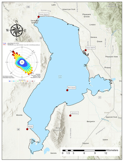
Figure 1.
AD sampling sites around and in Utah Lake and a wind rose showing the wind direction at the Provo Municipal Airport based on data from June 1990 to June 2021, generated by Iowa Environmental Mesonet (IEM), Iowa State University generated 2 June 2021 (https://mesonet.agron.iastate.edu, accessed 2 June 2021).
The three main concerns were:
- (1)
- Does the height of the sample table bias the measurements?
- (2)
- Does using a screen, which excludes insects and debris from the sample, make a difference on the measurements (despite not being a NADP rule or recommendation, the ULSP recommended small-mesh screens on the dry side bucket to prevent insects and plant debris from entering the sample), and
- (3)
- How well do measurements from the lake shore represent the deposition across the water surface?
While these questions are of interest to the ULSP and local stakeholders, they are also important to other AD research projects attempting to quantify the contribution of AD rates to the nutrient budget of lakes and reservoirs. These questions are critical in determining the nutrient budget and for developing valid Total Maximum Daily Load (TMDL) estimates designed to restore desirable conditions for lakes or reservoirs and particularly in the arid western US. Such questions are important in determining whether controllable sources of nutrients would be sufficient to meet TMDL or other management objectives.
This manuscript details the changes we made to address these concerns and how the changes affected the results. We modified the sampling tables to determine the effect that the sampler height had on AD measurements. We evaluated the effects on measured AD from a screen placed inside the sampling buckets to minimize insect intrusion or capture by the sampling. Earlier studies had assumed significant reduction in AD deposition rates across the lake. To quantify the deposition gradient, we installed a sampler on Bird Island (Figure 1), which is in the southern portion of Utah Lake near the center of an east–west transect line. Prevailing winds are generally in an NW–SE direction.
We constructed and placed the Bird Island station to evaluate assumptions about deposition gradients and analyze whether concentrations near the center of the lake were correlated with shoreline samplers. Previous studies [9,36] assumed different distribution patterns for AD on the lake with deposition rates decreasing to either background levels or zero deposition, respectively. The Bird Island sample location allowed us to collect data to better understand AD gradients and use more accurate assumptions for spatial interpolations to estimate total AD loads.
We used the information gained from this sample location to re-interpolate previous data to quantify the uncertainty in our previous estimates.
We will present the modifications we made to our sampling methods and procedures, then a statistical analysis to compare the effect of (1) sampler table heights, (2) screens in the sample buckets, and (3) an analysis of correlations among the shoreline and mid-lake sampler locations. Finally, we present an estimate of the total nutrient loads from AD for 2019 and 2020 and discuss the differences.
2. Materials and Methods
2.1. Sampling and Analysis Overview
To collect field samples, we followed the NADP sampling procedure using the details presented in Olsen, Williams, Miller and Merritt [9]. We collected samples weekly, acquiring both a wet-deposition sample and a dry-deposition sample from five sites in and around Utah Lake (Figure 1). As addressed in Olsen, Williams, Miller and Merritt [9], we simulated the dry-deposition collection properties of a wet lake surface by loading each dry-deposition sample bucket with 3 L of deionized water as recommended by Jassby, Reuter, Axler, Goldman and Hackley [7] and Anderson and Downing [6]. Each week, we replaced the field sample buckets with buckets that had been cleaned in an acid wash and rinsed with deionized water.
Figure 2 shows the sampling site at Mosida with both dry and wet deposition buckets. We collected samples from all five sites (Figure 1) using 500 mL clean Nalgene© wide-mouth amber HDPE bottles. Samples were analyzed by the Environmental Analytical Laboratory on the campus of Brigham Young University (https://pws.byu.edu/eal, accessed on 2 June 2021). We computed deposition rates as follows: we multiplied the nutrient concentration of each sample (mg/L) by the volume of the sample (L), which resulted in mg of nutrients deposited in the sample bucket. We used deionized water to bring samples up to analytical volume. We calculated unit area deposition rates by dividing the total deposition mass in milligrams for each sample by the surface area of the sample bucket (0.0615 m2) and the time represented by the sample (usually 1 week) following previous studies [9,36].
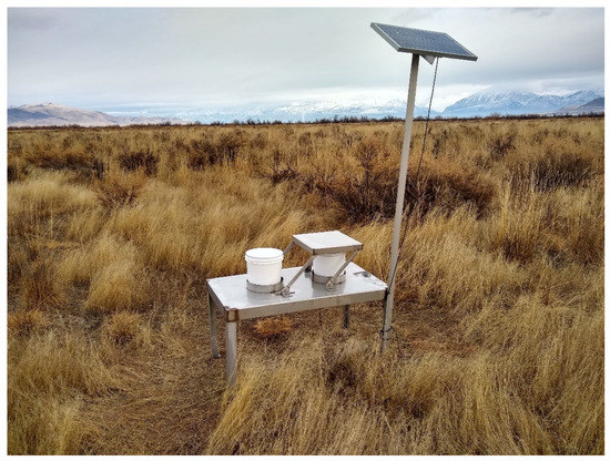
Figure 2.
The sampling site at Mosida showing the early design (1916–1919) of our sampling apparatus. When rain is detected, the lid transfers to close the dry deposition sample bucket and open the wet deposition sample bucket.
2.2. Sample Table Height
NADP guidelines for samplers require that the table should be 1 to 2 m from the ground. In our previous work, our tables were approximately 1.2 m from the ground, at the lower limit of the NADP guidelines. For the 2020 season, we raised the bucket height to 2 m to reduce the potential of near-ground transport from soil or vegetation that might not reach Utah Lake from entering the sample buckets.
To evaluate the effectiveness of raising the tables, we evaluated the data from the two locations with side-by-side tables (Figure 3). At each site, one table used the original 1.2 m table height, and one was at the new 2 m height (Figure 4). These tables were installed at the Central Davis Wastewater Treatment Plant location and the Ambassador Duck Club location (Figure 3). Both sites are located near Farmington, Utah for a similar study underway on Farmington Bay, part of the Great Salt Lake. We selected these sites as the sites were new, we were installing tables for sampling, and the general climate and landcover is similar to that around Utah Lake. This also provides data from an area different from Utah Lake to support generalizing the findings from this paper. Figure 3 shows the location of those samplers and Figure 4 shows a tall sampler next to a short sampler at the Ambassador Duck Club location.
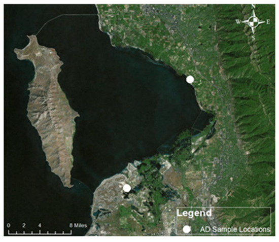
Figure 3.
Field locations that had side-by-side sample tables at ~1 m and ~2 m heights. These sample locations are near Farmington Bay on the Great Salt Lake approximately 50 km north of Utah Lake.
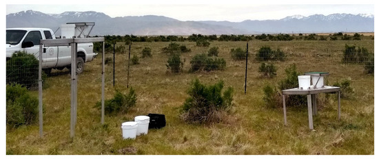
Figure 4.
High (~2 m) sample table on the left and the low (~1 m) sample table on the right.
2.3. Impacts of Screens on Samples
One of the major challenges for AD measurement near water involves sample contamination by insects, plant matter, or bird excrement [2,3]. Attempts have been made in other AD studies to solve this problem by installing additional samplers to increase the chance of collecting enough uncontaminated samples for analysis and locating the stations in areas less likely to have high insect populations [6]. Since we are attempting to measure AD to Utah Lake, our samplers need to be located near the shoreline and installing samplers in locations without significant insect populations is not possible. Tamatamah [10] explored limiting the impact of large outlier samples by removing contaminated samples, but this strategy leads to frequent missing data. There is no agreement on whether or not to include these local contaminants as part of the deposition as arguments could be made that insects and other contaminants are also deposited in the lake or conversely that these contaminants are only local and do not represent lake deposition [4].
Our earlier work included insects and other materials that were collected in the sample buckets as we reasoned these samples, including insects, represented contributions to the nutrient load on the lake [9,36]. However, including these contaminants—mostly insects—often resulted in large AD rates and was subject to criticism. Previously, we identified large amounts of insects, with the great majority being a terrestrial bee species Halictidae Lasioglossum, mostly at the Mosida location (Figure 5). For example, during the 2019 sampling year, from July to August, we counted approximately 100+ bugs per sample at the Mosida location in samples taken over a 4 week period.
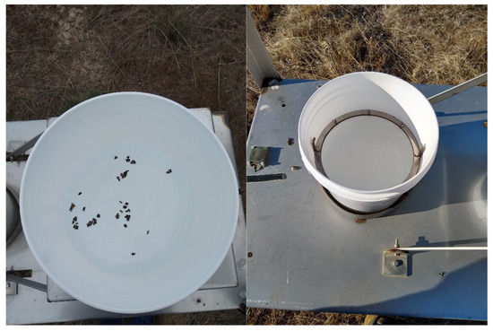
Figure 5.
A sample bucket at the Mosida site without screens after two days (left image) and with screens after one week (right image). The screens significantly lower the number of large objects in the sample.
To quantify the impact of including or excluding insects or other larger contaminants such as plant parts, we installed 500 micron mesh screens in each of the buckets for the 2020 year Figure 5. These screens exclude insects from being captured in the sample bucket. We immediately observed the impact of screens on the samples. For example, as shown in Figure 5, samples from the Mosida site had a significant number of insects in a sample period of only two days prior to installing the screen but had no insects for a sample period over a full week with the screens installed. We installed screens on each of our sample locations. After installing the screens, we saw no indication of large insects or plants in the samples. To quantify the difference between screened and unscreened samples, we performed a statistical analysis on 7 months of data that is reported later.
2.4. Bird Island Sampler
The largest concern with our previous sampling efforts and an issue that could arise when implementing AD sampling at other lakes or reservoirs is the assumption on the attenuation gradient in the rate of AD across a large lake, such as Utah Lake. Utah Lake has a small above water feature from hydrothermal processes called Bird Island. Bird Island is located in the south central portion of Utah Lake, as shown in Figure 2. We installed the AD sampler on the east side of Bird Island, as shown in Figure 6. The sampling table was slightly approximately 5 m above the lake surface. The sampler was secured by guywires and weights.
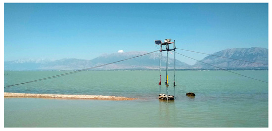
Figure 6.
The mid-lake sample location on the east side of Bird Island.
In addition to quantifying the AD gradient over the lake and addressing assumptions about the fall-off rates, we also evaluated whether we could estimate AD rates in the center of the lake only using shoreline samplers using traditional geospatial interpolation methods.
2.5. Other Modifications
2.5.1. Solar Panel Locations
One criticism of our sample table design was the location of the solar panel and associated support pole. The concern was that the solar panel and pole were too close to the samplers and could cause rain to deflect from the solar panel assembly and splash into the sample bucket, biasing the sample. We removed the solar panels and support pole from the sample table and moved the solar panel to a pole approximately 5 m from the sample table (Figure 7).
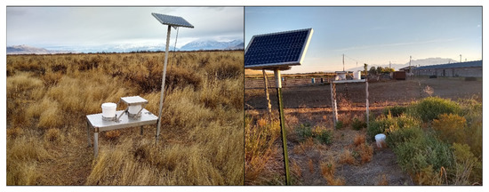
Figure 7.
Old solar panel installation shown in the right, with the new, modified installation moving the solar panel 5 m away from the sample table shown on the right.
2.5.2. Miners Moss Installation
A similar concern was raised about the sample table surface, which was smooth stainless steel. When a rain sensor detects moisture, the lid covering the wet deposition bucket is moved to cover the dry deposition bucket and expose the wet-side bucket. The concern was that during a rain event, there could be splash or bounce from the lid surface to the sample bucket. To address this issue, we glued miners moss on the lids. This can be seen as the green material on the bucket covering in Figure 4. NADP addressed this problem with their most recent design.
We performed some simple experiments to judge the effectiveness of the miner’s moss. We simulated heavy rainfall by pouring approximately 4 L of dyed water on the lid when it was situated on the dry side. Only a few milliliters reached the wet-side bucket, this visually confirmed that the miners moss absorbed the energy of raindrop impact and eliminated droplet splash or bounce that previously could have entered the wet sample buckets.
3. Results
3.1. High vs. Low Tables Comparison
We collected 38 pairs of data from the high–low table pairs over 8 months, collected from the Central Davis and Ambassador locations. This included 21 and 17 pairs from the Central Davis and the Ambassador site, respectively. To determine whether there were differences in the data collected at the different heights, we performed a paired t-test on these data pairs. In addition, we graphically evaluated that data using both time-history and box-and-whisker plots, as shown in Figure 8 and Figure 9, respectively.
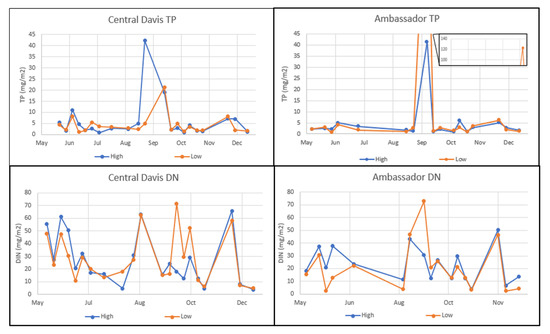
Figure 8.
A graphical comparison of TP data (top panel) and DIN data (bottom panel) collected over 8 months from paired high and low tables at two different sites, Central Davis and Ambassador, in the left and right panels, respectively. We did not remove any outliers from these data.
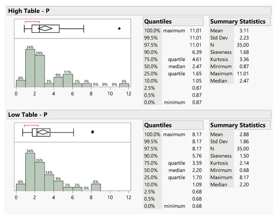
Figure 9.
Distributions and statistics of P data collected from the high table (top panel) and low table (bottom panel). Each panel includes a box-and-whisker plot (top left corner) a histogram (bottom left corner) and descriptive statistics (right side) for paired samples collected using a high or low table in the top and bottom panels, respectively. The distributions are skewed but have similar means and medians. Three outliers were removed. Data units are mg/m2.
In the box-and-whisker plot the line within the box represents the median sample value or the 50th quartile. The box ends represent the 25th and 75th data quartiles also expressed as the 1st and 3rd quartile, respectively. The diamond represents the mean and the upper and lower 95% of the mean as the center and left and right ends of the triangle, respectively. The size of the diamond is a visual representation of the size of the confidence interval. If the 50th quartile line is not in the center of the box or if the diamond is not centered on the 50th quartile line, then the data are skewed. The difference between the 1st and 3rd quartiles is called the interquartile range which is shown graphically on the plot and in the summary statistics. The lines that extend from the box, called whiskers, extend to the outermost data point that falls within:
- the 1st quartile − 1.5 × (interquartile range) and
- the 3rd quartile + 1.5 × (interquartile range).
If the data points do not reach these computed ranges, then the whiskers end at the upper and lower data point values (not including outliers). The red bracket outside the box identifies the shortest half, which is the densest 50% of the observations.
Figure 8 shows that visually, there is no correlation between table height and concentration. However, at the Central Davis location the low table seems to have slightly higher values during low deposition and higher values during high deposition, in contrast the plot of the data from the Ambassador site seems to exhibit the opposite trend. However, these patterns are not consistent even at a single site.
Figure 9 and Figure 10 show histograms, box-and-whisker plots, and descriptive statistics for data collected over 8 months in 2020 from the high and low paired collection sites for DIN and P, respectively. The box-and-whisker plots (top left corner of each panel) summarize the data distributions. The plots are on the same scale, so they can be compared visually. A visual comparison of both the P data and the DIN data, as shown in Figure 9 and Figure 10, respectively, show that the whisker plots appear very similar, with little differences between the distributions. This is a preliminary indication that the table height has no significant impact on the sample collection concentrations.
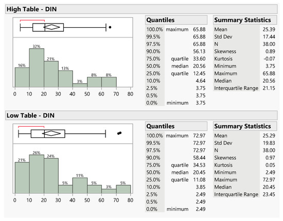
Figure 10.
Distributions and statistics describing DIN data collected from the high table (top panel) and low table (bottom panel). Each panel includes a box-and-whisker plot (top left corner) a histogram (bottom left corner) and descriptive statistics (right side) for paired samples collected using a high or low table in the top and bottom panels, respectively. The distributions are skewed but have similar means and medians. No outliers were removed. Data units are mg/m2.
Figure 9 and Figure 10 show that both the TP and DIN data are skewed by both the shape of the histogram and by the fact that the mean (center of the diamond) and the median (center of the box) are not aligned. The whisker plot is also asymmetric, another indication of a skewed distribution. The red brackets show that the densest region that contains 50% of the data is below the median value, but above the 25th quartile, indicating a data cluster.
The summary statistics, as shown in the right panels of Figure 9 and Figure 10, do indicate differences between the high and low table data with differences between both the mean and median values for the different data collection heights. We used several statistical tests to determine whether these differences in the mean values were significant.
Since we had paired measurements, e.g., measurements taken at the same location and time on both the high and low sampling tables, we used a paired t-test metric to determine whether the differences between the data collected from the high and low tables were significant.
The paired t-test compares two variables, one defines the paired setting for the measurements, in this case data collected at the high versus low table, the second variable is the measurement itself, in this case the measured deposition rate. We use the paired t-test to evaluate whether there is a difference between measurements taken at the high and low tables.
We selected a significance level of , where is the significance level, and then compared the t-test statistic to a t value from a standard chart or table based pm the degrees of freedom The resulting t value is written as , which for the P data with 34 measurements and is .
If the test statistic is lower than the t value, we cannot reject the null hypothesis that the mean difference is zero, so there is no statistical significance difference in the two datasets at the level which would indicated the measurements at the high and low table are not different at this significance level. If the test statistic is higher than the t value, then we reject the hypothesis that the mean difference is zero, and that means that the two sets of measurements are different.
Our data are well suited for this test because not only were the heights of the tables different, but each pair of measurements was collected at the same site at the same time.
Table 1 presents the results of the two-sided and one-sided paired t-tests on the P and DIN data. We performed the test using JMP® Pro, version 15.2.1 (SAS Institute, Inc., Cary, NC, USA). JMP reports the probability that, given for the P data, or for the N data, of observing a mean of the differences value greater than the observed value. Table 1 shows that the mean difference between the AD rates were 0.24 and 0.10 mg/m2 for the P and DIN data, respectively. For this dataset, the data collected by the high table was ~8% and ~0.3% higher than data from the low table for P and DIN, respectively.

Table 1.
Student t-test results comparing measurements from the collectors with high tables and low tables.
In Table 1, the column labeled presents the values for the two-sided t-test, presents values for the one-sided t-test on the high side, and presents results for the one-sided t-test on the low side. For both the two-sided (i.e., any difference in the mean difference) or one-sided tests which only look at the probability of exceeding the lower or upper bound, the probabilities are significantly higher than the value. We cannot reject the null hypothesis. These tests indicated that there is no statistical difference among the datasets.
We conducted a one-way ANOVA test with results almost identical to the two-sided t-test. The one-way ANOVA test also indicated no statistical difference between the two datasets. As the results were essentially identical to the values for the two-sided t-test, we did not include them in Table 1.
The data distributions are skewed, which for small datasets can affect the results of the t-test and the ANOVA test. To determine whether this affected the results, we performed the non-parametric (i.e., does not depend on the distribution) Wilcoxon/Kruskal–Wallis test, also known as the Mann–Whitney test, which evaluates rank-sums, it is resistant to outliers and does not require normality. For this test, we computed two-sided and one-sided probabilities greater than 0.95 for both datasets, values significantly higher than the 0.05 value we selected to test for significance.
The t-test and Wilcoxon/Kruskal test values for both P and DIN show that there is no statistical significance in the difference between data collected using a high or low table. These results do not prove that there is no difference, but the datasets are relatively large and collected occurred over an 8 month period which included periods of both high and low AD rates.
Based on this analysis, we can answer the criticism about the table heights. The data from the 1 m (low) tables are not statistically different than data from the 2 m (high) tables and we can use these data in our analysis.
3.2. Insects, Outliers and Screens
The second question we addressed was how screening the samples to exclude insects would affect the measured AD rates. There was some debate on this as insects do contribute to the lake AD loading. The issue is whether the sampling stations measured AD rates representative of the lake, or whether they only measured near-shore rates in specific locations. Visual examination of the samples indicated that certain stations, such as Mosida, had significantly more insects in the samples than others.
We previously addressed this issue by removing outliers in the data assuming that these outliers were caused by insect contamination. In 2020, we added screens to the sample buckets to exclude insects. This allows legitimate outlier samples, such as those caused by dust storms, to be included in the data.
We present this analysis in two parts. First, we compare data from all the sites, four in 2019 and five in 2020, with and without outliers included in the sample average. We present the results and discuss the differences and the impacts that removing the outliers has on the mean concentration calculations. Second, at two sites we installed sample buckets next to each other, one with a screen and one without. We statistically analyzed these paired data to describe and quantify the differences that a screen makes on the collected data.
3.2.1. Outlier Removal
At the end of May 2020, screens were added to the sample buckets. This means that the 2019 data were all collected without screens, but that approximately 7 months of 2020 data were collected with screens in place. This, importantly, included the summer months when insects are present. However, insects were present in both April and May before the screens were added.
We compared samples collected in 2019 and 2020 with and without outliers removed to better characterize the impact of outliers on AD concentrations. Historically and for this work, we considered a measurement an outlier if the concentration was greater than 1 mg/L for TP or 8 mg/L for DIN; these values are approximately 3 standard deviations above the mean for TP and DIN, respectively.
Table 2 presents the number of outliers and average weekly concentration with and without the outliers for 2019 and 2020. Table 2 shows that the majority of outliers occur at the Mosida site and are typically associated with large numbers of visible insects in the samples. The other outliers occur at the Lakeshore site and are also associated with insects.
Table 2.
A comparison of all the data with and without outliers removed from 2019 and 2020. This includes four and five stations for 2019 and 2020, respectively.
For TP samples at all sites in 2019 and 2020, there were 13 and 6 TP outliers, respectively. Of the six outlier samples in 2020, three occurred before screen installation. The remaining three outliers occurred during high wind days with large amounts of visible dust in the sample. For the DIN samples, all the sites in 2019 and 2020 had outliers. This includes the 2020 DIN data collected after screen installation.
Table 3 compares data taken at all the sample sites in 2019 and 2020 with and without outliers removed. The 2019 data for both TP and DIN, the mean concentrations for data with the outliers removed is approximately 15% of the concentration with the outliers included in the mean calculation. For 2020 data for both TP and DIN, the mean concentrations for data with the outliers removed is approximately 50% of the concentration with the outliers included in the mean calculation.
Table 3.
Comparison of the mean TP and DIN concentrations with and without outliers removed for the years 2019 and 2020. For part of 2020, screens were installed on the sample buckets.
These data show that outliers have a significant impact on the mean concentration, even though these outliers occur at only two sites, Mosida and Lakeshore. Though it is difficult to exactly quantify the impact of screens as they were not in place for all of 2020, the data show that screens affect both the number of outliers and the average concentration. While in 2019, the mean with outliers removed was only 15% of the mean of the data without the outliers removed, in 2020, it was 50%, significantly closer.
3.2.2. Screened vs. Unscreened Samples
We collected these data side by side over 6 months in 2020 at the Central Davis and Orem sites. Both the screened and unscreened samples were taken on 2 m tables. Between the two sites, Orem and Central Davis, there were 41 different pairs of samples collected, with 17 and 24 samples taken at the Central Davis and Orem sites, respectively.
The unscreened data generally had higher nutrient concentrations than the screened data. There are a few times when that is not the case; for example, in the largest discrepancy, the TP results from 10/29/2020 showed the screened Orem data to be 34.5 mg/m2 while the unscreened sampler at Orem for the same day was only 1.6 mg/m2. However, the results for most other samples showed the screened data to be lower in AD concentration than the unscreened data.
Figure 11 and Figure 12 show a graphical analysis and comparison of the distributions for the screened and unscreened TP and DIN data, respectively. This includes both a histogram and a box-and-whisker plot. The box-and-whisker plot is in the upper left of each panel, with a histogram plot in the lower left; descriptive statistics are included on the right. The histogram x-axis does not include the full range of the data to better present the data distribution in the lower range.
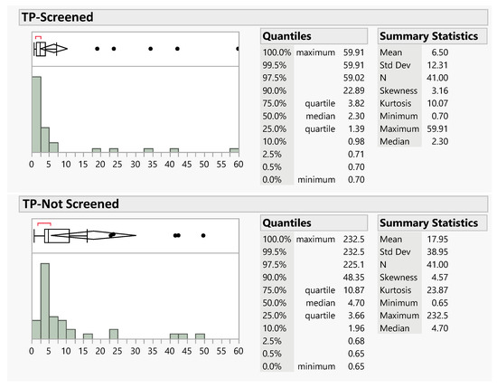
Figure 11.
Distributions and summary statistics for the screened and unscreened TP samples collected side by side. The x-axis does not include the full range of the data to better show detail in the lower range. Data units are mg/m2/week.
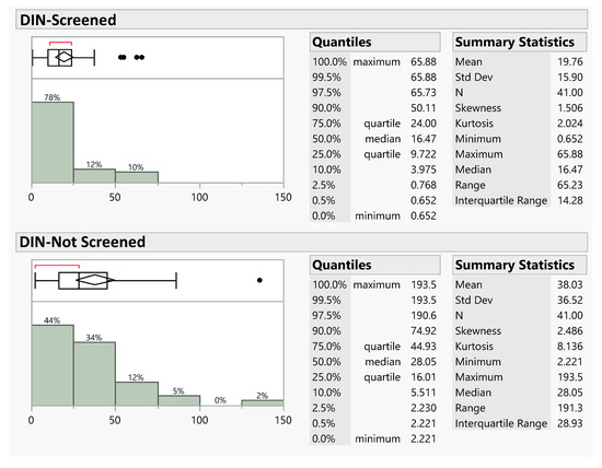
Figure 12.
Distributions and summary statistics for the screened and unscreened DIN samples collected side by side. The x-axis does not include the full range of the data to better show detail in the lower range. Data units are mg/m2/week.
For both the TP data (Figure 11) and the DIN data (Figure 12), the graphical plots show large differences in the distributions. For the two panels in each figure, the x-axis is the same scale allowing a direct visual comparison of the box-and-whisker plot.
The paired TP data for data collected by either the screened or unscreened samples are highly skewed, with almost no overlap between the 95% confidence interface for the mean value and the quantile box representing the range from the 25th to 75th quantiles. The box sizes are also very different, with the data taken from the unscreened sampler having a much larger range than the range of the data taken with the screened sampler. This is quantified by the summary statistics where the range of the data is ~60 and ~230, and the interquartile range is ~2.5 and ~7.2 for the data taken with the screened and unscreened samplers, respectively.
The paired DIN data show very similar trends to the TP data. Both data distributions are significantly skewed, and there is minimal overlap between the boxes in the box-and-whisker plots. The summary statistics show large differences between the data range of ~65 and ~190 with an interquartile range of ~14 and ~29 for the data collected by the screened and unscreened samplers, respectively.
We compared the differences in the mean concentrations of TP and DIN using a paired t-test. Since the distributions were so skewed, we applied a natural log transformation on the data before performing the test. We used the one-sided p-value for reference since the hypothesis was directional. We analyzed the paired data using JMP Pro®. The log of the average difference between screened and unscreened TP data was 0.823, with a 95% confidence interval of 0.398 to 1.249, the t-test gave a p-value of 0.0018. We back transformed these data and found that the multiplicative difference in the means is 2.488, with a 95% confidence interval of 1.488 to 3.488. For DIN, the log of the average difference was 0.555 with a 95% confidence interval of 0.266 and a p-value of 0.0116. The back-transformed multiplicative difference in the means was 1.816 with a 95% confidence interval of 1.305 to 2.326.
The p-values of 0.0018 and 0.016 for the paired P and DIN data, respectively were well below the 0.05 significance level indicates that there is a statistically significant difference between the data taken using screened and unscreened samplers. The unscreened samples in mg/m2 had on average 3-fold the amount of TP as the screened samples. There is moderate evidence for a difference in the amount of DIN, with the unscreened samples having 1.5-fold the amount of the screened samples.
The data show that installing screens on the samplers provided a barrier to contamination (e.g., insects or vegetation). There is still some debate on whether these contributions should be part of the sample or not. However, excluding these nutrient sources from load calculations will result in computed loads below actual loads for this method as we know that both insects and other large particles do contribute to AD deposition rates. However, these large-particle sources probably do not extend significant distances into the lake. The screened samples provide a conservative (lower) estimate of AD at a location.
3.3. Lake Interior Measurements
The third question we attempted to answer was our assumptions on the behavior of the AD gradient across the lake. We received initial feedback and assumed that deposition rates would decrease rapidly away from the shore. This was based on the general understanding of local dust sources. As we discussed, local dust source deposition rates decrease dramatically with distance, though this fall-off is attributed to that fact that the majority of the initial dust loads are larger particles that settle rapidly [33,34,35]. These same studies show that the smaller dust fractions are much lighter, have slow settling rates, and can be transported over large distances. This type of transport is what we are attempting to quantify with shoreline stations located away from local point dust sources and a station placed in the interior of the lake to evaluate longer-distance transport.
We placed a measurement station on the interior of the lake (Figure 1) at Bird Island (Figure 6) to characterize the spatial distribution and falloff of AD on Utah Lake. We wanted to determine whether AD rates measured on the lake shore significantly decreased in the lake interior. The Bird Island sampler was placed at least 2 m above the ground/lake level, though at lower lake levels it was slightly higher (Figure 6). The lips of the sample buckets are approximately 0.5 m higher than the table. This helped isolate the sampling buckets from water spray.
The results from 2020 show that samples taken at the Bird Island location generally had higher nutrient AD concentrations than samples collected at the shoreline samplers. Over the 5 months that the Bird Island sampler was available (July to November), it had a higher or approximately the same AD concentration as the shoreline samplers. There was a single data point where the shoreline sampler, Pump Station, on 9 April 2020 that was higher than the Bird Island sampler. Figure 1 shows that prevailing winds would generally carry dust from the north-west shoreline area or the south-east area, neither of which have shoreline samplers. The wind rose is based on over 10 years of data. The north-west shoreline is a potential large dust source based on our experience.
These results run contrary to our previous assumption that AD deposition rates decrease rapidly away from the shore. This assumption was based on guidance we received [37]. In retrospect, we believe that the measurements used to support this assumption, which were made at two points, one near an unpaved road and the second on a boat located in the lake just off the shore from the road, measured the initial fall-off of the larger particles mobilized by the road traffic which is consistent with published patterns [32,33]. We believe our shoreline samples are measuring rates similar to those measured by the boat which consist of finer particles that can be transported over longer distances. We place our shoreline samplers away from trafficked unpaved roads, and we believe the measurements at these locations are not affected by these larger particles and measure smaller suspended dust particles that can be transported several kilometers without significant decrease in deposition rates depending on wind speeds. Our data showed that the deposition rates measured by the shoreline samplers continue over the lake with little change based on the Bird Island data supporting this hypothesis.
Table 4 and Table 5, which have TP and DIN monthly deposition rates, respectively, indicated that AD rates measured at the Bird Island sampler are generally higher than those measured at shoreline samplers except for two measurements. The Bird Island site measured a lower TP AD rate than the average of the shoreline samplers in October of 2020, approximately 64% lower than the average AD rate for TP measured at the shoreline samplers. The Bird Island sampler measured a lower AD rate for DIN in August of 2020, 19% lower than the August 2020 average AD rate of DIN for the shoreline samplers. Past assumptions were that AD rates decrease significantly from the shore samplers to the middle of the lake and nutrient load estimates were based on these assumptions [9,36]. Data collected at Bird Island show that these assumptions were incorrect, that mid-lake deposition rates are similar to those measured by shoreline samplers.
Table 4.
Monthly TP deposition data comparing results from the lake interior sampling location (Bird Island) to data from lake shore sample locations. Except for October, Bird Island, the lake interior site, had higher AD rates than the average of the four shoreline sites. All data represent deposition rates in mg/m2/month.
Table 5.
Monthly DIN deposition data comparing results from the lake interior sampling location (Bird Island) to data from lake shore sample locations. Except for August, Bird Island, the lake interior site, had higher AD rates than the average of the four shoreline sites. All data represent deposition rates in mg/m2/month.
Figure 1 shows that Bird Island would be most influenced by shoreline rates from the northwest shore of Utah Lake and the area north of the Mosida sampling site. Neither of these areas have a shoreline sampler. The northwest shore area is does not have much agriculture and is potentially a larger dust source. We hypothesize that Bird Island results would correlate with those from a sampler on the northwest shoreline. We are exploring the possibility of placing a sampler in this area for future collections.
3.4. Mid-Lake and Shoreline Sampler Correlations
To characterize the relationship between the data measured mid-lake at the Bird Island location with the shoreline samplers, we performed a general linear F-test. We used the test to determine whether there was a relationship among four the shoreline sites and the Bird Island location. The general linear F-test attempts to predict the Bird Island results using data from the shoreline samplers. We examined both a full model which uses all four shoreline sample sites to predict the Bird Island sampler results and reduced models created by removing each sample sites sequentially [38]. We used JMP Pro® to create and evaluate the models using the extra sum of squares test. We used log-transformed data because of the skewed distribution.
As expected, the full model most accurately predicted TP deposition rates at Bird Island using data from all four shoreline sites. Analysis indicated that the model was influenced by outlier observations. Normally these outliers would be removed from the model development however, considering that there are only 16 samples available we did not remove any data points from the model. The TP models indicated that there is some evidence for Lakeshore (p-value 0.0308) and for Orem (0.0323) AD rates being related to Bird Island TP. The Pump Station TP rates have a lower p-value (0.0124) indicating better predictive power even though those two sites are the furthest apart. The Mosida site did not indicate any strong statistical evidence for a linear relationship to Bird Island TP (0.0880).
The data are consistent with the wind rose, as shown in Figure 1. While Pump Station is one of the furthest samplers from Bird Island and Mosida is closer and, based on observations, a more likely dust source because of playa deposits, the wind rose, as shown in Figure 1, shows that prevailing winds align with the Bird Island-Pump Station axis, while prevailing winds do not generally connect Bird Island and the Mosida samplers.
The DIN model analysis showed that there is not strong evidence that any of the sites are linearly related with Bird Island, all the p-values were greater than 0.450. There is no strong statistical evidence that Lakeshore, Orem, Pump Station, and Mosida are linearly related for DIN to Bird Island.
3.5. Monthly Average Analysis
We computed and compared average monthly AD rates from 2017 to 2020 to understand monthly variation and variations between pre-screened and post-screened samples. For each site, we computed a monthly average from the measured weekly AD, as shown in Figure 13 for TP and DIN, respectively. We also computed a monthly average by averaging each of the site values. These results are presented in Table 6 and Table 7 for the TP and DIN data, respectively.
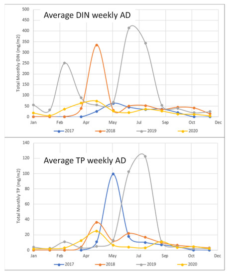
Figure 13.
Monthly average of weekly AD for DIN and TP in the top and bottom panels, respectively. Values are in mg/m2/week.
Table 6.
Monthly average of weekly DIN AD (mg/m2/week) 1.
Table 7.
Monthly average of weekly TP AD (mg/m2/week) 1.
Both the figures and tables show that adding screens to the sample buckets in 2020 had a significant impact on the summer data. In 2017 and 2019, Figure 13 shows spikes of TP occurring in May and July, respectively, while the 2020 data never showed a spike with a similar magnitude. The only spike occurring in May before the screens were installed. Adding screens to the collection buckets seemed to be the major change, as the 2020 non-summer months have data similar to the other years.
4. Estimated Utah Lake Atmospheric Deposition
4.1. Previous Approach
The objective of this research is to estimate the nutrient loads to Utah Lake from AD sources. This requires us to calculate the spatial AD rates for specific sample dates, then integrate those rates over time to compute the total annal loads. In this paper, we specifically address shortcomings and concerns that were raised with previous estimates. In this section, we provide a brief discussion of previous load estimates and how they were computed to better describe the improvements and place them in context.
In 2017 Olsen, Williams, Miller and Merritt [9] assumed that AD rates decreased significantly away from the shore, with AD rates at the center of the lake matching background long-range transport estimates. To estimate the total load to the lake, they added 5 hypothetical locations inside the lake and assumed background AD rates of 0.019 mg m−2 day−1 at these locations [9]. They then used ordinary kriging to compute the spatial distribution across the lake at each sample time, then integrated those spatial maps through time to estimate the total load. Reidhead [36], rather than using kriging or other standard geo-spatial statistical methods, used an interpolation method that assumed linear fall-off of AD rates away from the shore, with deposition rates assumed to be zero at the center of the lake [36].
Based on the results from the Bird Island sample location, both these previous assumptions are too conservation. Our data show that mid-lake deposition rates do not approach zero or background rates, but instead are the same magnitude and similar to shoreline data.
4.2. Nutrient Load Estimation Methods
We used ordinary kriging (OK) as implemented in Arc GIS Pro® with a standard variogram to interpolate among the four sample points for 2019 and the five sample points for 2020. We followed the methods of Olsen [9] but, as discussed above we have a better understanding of deposition distribution rates across the lake. In previous estimates, the AD rates were assumed to approach either zero or background near the lake center. With our better understanding of AD rates, we know that AD rates are relatively consistent over the lake, so for 2019 data, we applied OK using the four lakeshore sample points without pseudo points used previously to force rates at the center of the lake to lower values. For 2020, we used data from the five sample locations, including Bird Island in the center of the lake. We also estimated Bird Island data for months without measurements with details described later. This improved method uses lake interior AD rates higher than those used in previous years, but supported by data.
For 2019 data, we used OK to interpolate the spatial distribution of AD for each sample using data from the four lakeshore sample sites. We used a different approach for the 2020 data. For the 5 months of 2020 (July to November) during which we had data from Bird Island, we used OK and data from all 5 sites to estimate spatial distributions. For the other 7 months 2020 (January to May and the month of December) we estimated Bird Island AD rates using the regression equations generated from the statistical analysis described above. In situations where the model estimation resulted in a negative value or a value that did not fit with other data, we used the mean of the four sites, rather than the model predicted value. This was rare. We did not attempt to estimate Bird Island data for 2019, we just assumed a continuous spatial distribution as computed by the OK approach.
For both 2019 and 2020, we did impute missing values at any given site. If a site was missing a measurement for a given week, we estimated the missing value as the average of the other sites for that week. If a site measurement appeared to be an outlier, we excluded that value and only used the remaining sites in computing the average.
Once we had a complete dataset for 2019 (4 sites) and 2020 (5 sites), we loaded the data into ArcGIS Pro®. Using ArcGIS, we used the Kriging tool to generate a raster layer that represented the AD rates for that week. We computed a raster for each week in 2019 and 2020. We then applied a mask to only select the cells within the Utah Lake boundary. These rasters represented AD rates in mg/m2/week. We then multiplied the raster by the lake area to obtain the total weekly deposition, then summed these data to estimate the total annual deposition. We completed these steps for both TP and DIN. For convenience, we converted the results from milligrams/year to tons/year.
As discussed, even though the linear regression performed on the Bird Island sampler compared with the other samplers did not return strong evidence that the Bird Island AD could be predicted by the other samplers, we used the results from the regression analysis for 2020 because we felt it better represented full lake AD.
4.3. Estimated Utah Lake Nutrient AD
Figure 14 shows a map of interpolated DIN for the week of 23 August 2020. This is an example as similar interpolations were computed for each week in 2020 for both DIN and TP using measured data at the shoreline sites and measured and imputed data at the Bird Island site as described. The interpolation and calculation for 2019 followed the same process, except using only measured data at the four sample points around the lake used for the interpolation. We did not estimate Bird Island data for 2019.
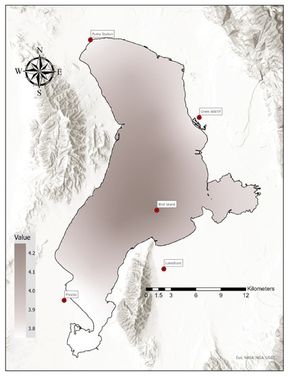
Figure 14.
Interpolated DIN AD results on 23 August 2020, using the five sampler locations including the Bird Island in the lake interior. For this week, Bird Island and Lakeshore had similar values, while the other stations were lower.
Figure 14 and visual examination of other interpolation maps clearly indicate that the addition of a sampler on the west side of the lake would be beneficial for spatial interpolation.
Table 8 shows estimated total annual TP loads of 262 and 133 tons for 2019 and 2020, respectively with total annual DIN loads of 1052 and 482 tons for 2019 and 2020, respectively. One potential reason that the 2019 data are larger than the 2020 data are that the 2020 data were from screened sampler buckets that excluded insect contributions to the data.
Table 8.
Total annual AD nutrient loads to Utah Lake for 2019 and 2020.
Figure 15 shows the weekly loads of TP and DIN for 2020 and 2019 in the top and bottom panels, respectively. The figure shows that there is significant seasonal variation in both years. In general, the winter months had minimal AD loads with maximum AD occurring during the summer. The 2019 data are higher than the 2020 data, but as noted, the 2019 data were from unscreened sample buckets. In addition, the large spike in the 2020 data occurred in May prior to screen installation. As we discussed, these large peaks are most likely the result of contributions from large numbers of insects in the samples. With screened sample buckets, the 2019 data would probably be similar to the 2020 data collected after June, with peaks significantly lower.

Figure 15.
Weekly for DIN and TP AD for 2020 and 2019 in the top and bottom panels, respectively.
5. Discussion
5.1. Sample Table Height and Modifications
Our data showed, using two different statistical tests, that there no statistically significant difference between datasets collected at side-by-side high or low tables for either TP or DIN. The lower buckets had, on average, slightly smaller concentrations of both nutrients than the higher buckets; the opposite of what our original hypothesis stated. Based on these results, we will continue to use 1 m tables, at the lower end of the NADP recommended range. These results also justify being able to mix table collected from tables at either height, though we recommended using a standard table height for a given example.
We evaluated moving the solar power panels away from the sample tables and covering the sample tables with miner’s cloth. Both these modifications were suggested to reduce the chance for splash to influence sample results. We did not test these two modifications separately, but neither modification showed observable differences in the collected data. Our results withstanding, we recommend placing the solar panel or other infrastructure away from the sampling table to minimize the possibility of issues. While our results did not show any observable difference, it is easy to identify scenarios where impacts could occur that would not have been captured in our dataset, that is why we recommend separating infrastructure. The use of miner’s cloth is more ambiguous, we feel that impacts from table surface splash are significantly less likely. However, it is a small modification. We did not modify our other tables because of the lack of impact we observed and the expense of modifying existing experimental apparatus.
5.2. Sample Bucket Screens
Our data showed that samples from screened buckets had significantly less nutrients than samples from unscreened buckets. The monthly comparison demonstrated that the 500 micron mesh screens prevented contamination (bugs, local vegetation, etc.) in the samples with a significant different in the results.
In addition to the experiment designed to evaluate the impact of screens, we analyzed monthly deposition patterns from 2017 through 2020. The data collected up through May 2020 were from unscreened sample buckets. The data after May 2020 were from screened buckets. In the early data from unscreened buckets, collected from 2017 through the 2019, the summer data showed significant concentration spikes, up to 10-fold the yearly average AD values. The later data from screened sample buckets only had spikes approximately 3-fold the yearly average of AD. For example, the Central Davis site for 2020 had side-by-side measurements where we had co-collected samples from screened and unscreened buckets. For this site, the November sample had DIN deposition values of approximately 135 and 60 mg/m2 for unscreened and screened sample buckets, respectively, approximately a 225% reduction.
Our analysis did not address the question of whether the screened or the unscreened bucket samples are the most accurate representation of total AD as insects and other debris are deposited onto the lake surface. Samples from screened buckets might underrepresent actual deposition rates, while samples from unscreened buckets may overestimate actual deposition rates. In either case, the samples from the screened buckets provide a conservative (lower) estimate of total nutrient loads.
5.3. Deposition Patterns and Spatial Distributions
Previously we assumed that AD rates would decrease significantly away from the shore. We placed a sample location in the interior of Utah Lake at Bird Island to explore this assumption. We found that there was no evidence for deposition rates decreasing away from the shore. In most samples, the Bird Island values were higher than many of the shoreline samples. We expect that this is because of prevailing winds, with the lake interior AD rates being most closely related to the upwind sample site.
We evaluated the correlation between AD nutrient concentrations at the four shoreline sites and those measured at the Bird Island site. We used both reduced and full statistical regression models, though there were only 16 co-collected observations. We found that while the data among the sites were similar, the models were only minimally successful in predicting Bird Island concentrations with r-squared values on the order of 0.6.
One unexplored variable in this analysis is the impact of wind directions, and the correlations among the sites vary, depending on instantaneous winds and how they affect the transport of AD. The wind rose at the Provo Airport, as shown in Figure 1, computed from data from 1990 to 2021, over 10 years of data, showed prevailing winds along the NE–SW line, with winds both from the NE and from the SW in almost equal amounts. This significantly affects correlations among the sites.
Based on our results, we demonstrated that we could use either the four shoreline sites or all five sites, including the lake interior site, to interpolate the spatial distribution of nutrient AD rates. That we did not need to assume that rates significantly decreased away from the shoreline. More accurate estimates could be made with additional shoreline and lake interior stations, with the highest priority being on the west side of the lake.
5.4. Updated AD Nutrient Loads
Based on our findings, we updated estimates for nutrient loads in 2019 and 2020. For 2019, we only used the four shoreline stations, and for 2020, we used the four shoreline stations and measured Bird Island data for 5 months and estimated Bird Island data for the remaining 7 months. We estimated that there were approximately 262 and 133 tons of TP added to Utah Lake in 2019 and 2020, respectively. We estimated that 1052 and 482 tons of DIN were added to Utah Lake in 2019 and 2020, respectively. All the 2019 data and the 2020 data prior to June were collected from unscreened sample buckets. Dry deposition represents the majority of deposition [9].
6. Analysis and Conclusions
This research was designed to address three main issues associated with measuring total AD of nutrients to water bodies:
- (1)
- Does the height of the sample table bias the measurements?
- (2)
- Does using a screen, which protects the samples from bugs and debris, make a significant difference on the measurements?
- (3)
- How well do measurements from the lake shore represent the deposition across the water surface?
To address these issues and concerns, we used data from an on-going study of nutrient AD at Utah Lake and data collected in 2020 specifically to address these issues. We applied our findings to update nutrient load estimates for both DIN and TP for the 2019 and 2020 calendar years.
While the data we present are specific to Utah Lake, the general approach, methods, and understandings are useful to water managers and researchers at other locations.
We found no significant difference between data collected using 1 m or 2 m tables. These heights represent the extremes of the recommended NADP sample table heights. We showed that samples taken from screened buckets were significantly different than samples from unscreened buckets, with the largest differences in the spring and summer because of insect contributions to the unscreened bucket samples. We did not attempt to determine which method better represents total loads to the lake, as insects can provide a significant portion of the load, but our data showed that the difference between screened and unscreened samples was very location specific, with two sites showing very large differences. Based on these results, we recommend using screens on sample buckets and have modified all our samplers.
To estimate nutrient loads, previous studies assumed that deposition decreased to either zero or background levels away from the shore. Our data showed that even on a lake as large as Utah Lake, approximately 15 by 35 km, deposition rates did not decrease away from the shoreline. We recommend that managers and researchers estimate spatial deposition distributions using available data, even if all the data are measured at shoreline locations, there is no need to assume that deposition rates decrease.
Based on our findings, we re-estimated nutrient loads for 2019 and estimated loads for 2020. The 2019 estimated loadings were significantly higher than those for 2020. We attribute this to the use of samples from unscreened buckets. We argue that the 2020 results represent the low range for AD nutrient loads while those for 2019 represent the high range. An analysis of monthly average data from 2017 through 2020 showed that with the exception of spikes in the summer months in the data prior to 2020, all four years exhibited similar deposition patterns in time. The spikes significantly affect the annual loads and based on their occurrence in the spring and summer months, can be attributed to insects and other debris. Nutrient AD rates are highest in the summer season at Utah Lake, which coincides with the periods of peak algal growth. This is the period of highest uncertainty because of the issue of whether or not to include insect contributions to the nutrient loads. This will require additional research, and a much denser sample network, to address.
Using our updated methods and assumptions, we found that AD nutrient loads alone are sufficient to cause significant algal growth in Utah Lake and cause eutrophic conditions on the lake. While this study was specific to Utah Lake, this analysis should be a foundation on which water managers at other locations could use as reason to start their own AD monitoring project.
Author Contributions
Conceptualization, M.B.B., T.G.M., A.W.M., L.B.M., and S.M.B.; methodology, T.G.M., D.C.R., S.M.B., L.B.M., and A.W.M.; software, S.M.B. and G.P.W.; investigation, S.M.B. and G.P.W.; resources, T.G.M. and A.W.M.; data curation, S.M.B. and D.C.R.; writing—original draft preparation, G.P.W.; writing—review and editing, A.W.M., M.B.B., T.G.M., L.B.M. and D.C.R.; visualization, S.M.B. and G.P.W.; supervision, T.G.M. and A.W.M.; project administration, T.G.M. All authors have read and agreed to the published version of the manuscript.
Funding
This research received no external funding.
Acknowledgments
We would like to acknowledge Brigham Young University, the South Davis Sewer District, and Chemtech-Ford for supporting this work.
Conflicts of Interest
The authors declare no conflict of interest.
References
- Uttormark, P.D.; Chapin, J.D.; Green, K.M. Estimating Nutrient Loadings of Lakes from Non-Point Sources; U.S. Government Printing Office: Washington, DC, USA, 1974.
- Newman, E. Phosphorus inputs to terrestrial ecosystems. J. Ecol. 1995, 83, 713–726. [Google Scholar] [CrossRef]
- Ahn, H.; James, R.T. Variability, Uncertainty, and Sensitivity of Phosphorus Deposition Load Estimates in South Florida. Water Air Soil Pollut. 2001, 126, 37–51. [Google Scholar] [CrossRef]
- Graham, W.F.; Duce, R.A. Atmospheric Pathways of the phosphorus cycle. Geochim. Cosmochim. Acta 1979, 43, 1195–1208. [Google Scholar] [CrossRef]
- Hicks, B.B. Measuring dry deposition: A re-assessment of the state of the art. Water Air Soil Pollut. 1986, 30, 75–90. [Google Scholar] [CrossRef]
- Anderson, K.A.; Downing, J.A. Dry and wet atmospheric deposition of nitrogen, phosphorus and silicon in an agricultural region. Water Air Soil Pollut. 2006, 176, 351–374. [Google Scholar] [CrossRef]
- Jassby, A.D.; Reuter, J.E.; Axler, R.P.; Goldman, C.R.; Hackley, S.H. Atmospheric deposition of nitrogen and phosphorus in the annual nutrient load of Lake Tahoe (California-Nevada). Water Resour. Res. 1994, 30, 2207–2216. [Google Scholar] [CrossRef]
- Lehmann, C.M.B.; Gay, D.A. Monitoring long-term trends of acidic wet deposition in US precipitation: Results from the National Atmospheric Deposition Program. Power Plant Chem. 2011, 13, 378–385. [Google Scholar]
- Olsen, J.M.; Williams, G.P.; Miller, A.W.; Merritt, L.B. Measuring and Calculating Current Atmospheric Phosphorous and Nitrogen Loadings to Utah Lake Using Field Samples and Geostatistical Analysis. Hydrology 2018, 5, 45. [Google Scholar] [CrossRef] [Green Version]
- Tamatamah, R.A.; Hecky, R.E.; Duthie, H.C. The atmospheric deposition of phosphorus in Lake Victoria (East Africa). Biogeochemistry 2005, 73, 325–344. [Google Scholar] [CrossRef]
- Prospero, J.; Glaccum, R.; Nees, R. Atmospheric transport of soil dust from Africa to South America. Nature 1981, 289, 570–572. [Google Scholar] [CrossRef]
- Duce, R.A.; Unni, C.; Ray, B.; Prospero, J.; Merrill, J. Long-range atmospheric transport of soil dust from Asia to the tropical North Pacific: Temporal variability. Science 1980, 209, 1522–1524. [Google Scholar] [CrossRef] [Green Version]
- Cole, J.J.; Caraco, N.F.; Likens, G.E. Short–range atmospheric transport: A significant source of phosphorus to an oligotrophic lake. Limnol. Oceanogr. 1990, 35, 1230–1237. [Google Scholar] [CrossRef]
- Lewis, W.M., Jr. Precipitation chemistry and nutrient loading by precipitation in a tropical watershed. Water Resour. Res. 1981, 17, 169–181. [Google Scholar] [CrossRef]
- Schindler, D.; Newbury, R.; Beaty, K.; Campbell, P. Natural water and chemical budgets for a small Precambrian lake basin in central Canada. J. Fish. Board Can. 1976, 33, 2526–2543. [Google Scholar] [CrossRef]
- Stockdale, A.; Krom, M.D.; Mortimer, R.J.; Benning, L.G.; Carslaw, K.S.; Herbert, R.J.; Shi, Z.; Myriokefalitakis, S.; Kanakidou, M.; Nenes, A. Understanding the nature of atmospheric acid processing of mineral dusts in supplying bioavailable phosphorus to the oceans. Proc. Natl. Acad. Sci. USA 2016, 113, 14639–14644. [Google Scholar] [CrossRef] [PubMed] [Green Version]
- Kopàček, J.; Hejzlar, J.; Vrba, J.; Stuchlík, E. Phosphorus loading of mountain lakes: Terrestrial export and atmospheric deposition. Limnol. Oceanogr. 2011, 56, 1343–1354. [Google Scholar] [CrossRef]
- Peters, R.H. The role of prediction in limnology 1. Limnol. Oceanogr. 1986, 31, 1143–1159. [Google Scholar] [CrossRef]
- Zhai, S.; Yang, L.; Hu, W. Observations of atmospheric nitrogen and phosphorus deposition during the period of algal bloom formation in Northern Lake Taihu, China. Environ. Manag. 2009, 44, 542–551. [Google Scholar] [CrossRef] [PubMed]
- Merritt, L.B.; Miller, A.W. Interim Report on Nutrient Loadings to Utah Lake: 2019; Jordan River, Farmington Bay & Utah Lake Water Quality Council: Provo, UT, USA, 2019. [Google Scholar]
- Carlson, R.E. A trophic state index for lakes 1. Limnol. Oceanogr. 1977, 22, 361–369. [Google Scholar] [CrossRef] [Green Version]
- PSOMAS. Utah Lake TMDL: Pollutant Loading Assessment & Designated Beneficial Use Impairment Assessment; Utah Division of Water Quality: Salt Lake City, UT, USA, 2007.
- Abu-Hmeidan, H.Y.; Williams, G.P.; Miller, A.W. Characterizing total phosphorus in current and geologic utah lake sediments: Implications for water quality management issues. Hydrology 2018, 5, 8. [Google Scholar] [CrossRef] [Green Version]
- Randall, M.C.; Carling, G.T.; Dastrup, D.B.; Miller, T.; Nelson, S.T.; Rey, K.A.; Hansen, N.C.; Bickmore, B.R.; Aanderud, Z.T. Sediment potentially controls in-lake phosphorus cycling and harmful cyanobacteria in shallow, eutrophic Utah Lake. PLoS ONE 2019, 14, e0212238. [Google Scholar] [CrossRef] [PubMed]
- Larsen, D.; Mercier, H. Lake phosphorus loading graphs: An alternative. Natl. Tech. Inf. Serv. 1975, PB-243 869, 4. [Google Scholar]
- Merritt, L.B.; Miller, A.W. Interim Report on Nutrient Loadings to Utah Lake; Jordan River, Farmington Bay & Utah Lake Water Quality Council: Provo, UT, USA, 2016. [Google Scholar]
- Lamb, D.; Bowersox, V. The national atmospheric deposition program: An overview. Atmos. Environ. 2000, 34, 1661–1663. [Google Scholar] [CrossRef]
- Wetherbee, G.A. Precipitation collector bias and its effects on temporal trends and spatial variability in National Atmospheric Deposition Program/National Trends Network data. Environ. Pollut. 2017, 223, 90–101. [Google Scholar] [CrossRef] [Green Version]
- Nanus, L.; Campbell, D.H.; Ingersoll, G.P.; Clow, D.W.; Mast, M.A. Atmospheric deposition maps for the Rocky Mountains. Atmos. Environ. 2003, 37, 4881–4892. [Google Scholar] [CrossRef]
- Goodman, M.M.; Carling, G.T.; Fernandez, D.P.; Rey, K.A.; Hale, C.A.; Bickmore, B.R.; Nelson, S.T.; Munroe, J.S. Trace element chemistry of atmospheric deposition along the Wasatch Front (Utah, USA) reflects regional playa dust and local urban aerosols. Chem. Geol. 2019, 530, 119317. [Google Scholar] [CrossRef]
- Ginoux, P.; Prospero, J.M.; Gill, T.E.; Hsu, N.C.; Zhao, M. Global–scale attribution of anthropogenic and natural dust sources and their emission rates based on MODIS Deep Blue aerosol products. Rev. Geophys. 2012, 50. [Google Scholar] [CrossRef]
- Zhao, G.; Chen, Y.; Hopke, P.K.; Holsen, T.M.; Dhaniyala, S. Characteristics of traffic-induced fugitive dust from unpaved roads. Aerosol Sci. Technol. 2017, 51, 1324–1331. [Google Scholar] [CrossRef]
- Veranth, J.M.; Pardyjak, E.R.; Seshadri, G. Vehicle-generated fugitive dust transport: Analytic models and field study. Atmos. Environ. 2003, 37, 2295–2303. [Google Scholar] [CrossRef]
- Chow, J.C.; Watson, J.G.; Green, M.C.; Lowenthal, D.H.; DuBois, D.W.; Kohl, S.D.; Egami, R.T.; Gillies, J.; Rogers, C.F.; Frazier, C.A. Middle-and neighborhood-scale variations of PM10 source contributions in Las Vegas, Nevada. J. Air Waste Manag. Assoc. 1999, 49, 641–654. [Google Scholar] [CrossRef] [PubMed] [Green Version]
- Peden, M.E. Sampling, analytical, and quality assurance protocols for the National Atmospheric Deposition Program. In Sampling and Analysis of Rain; ASTM International: West Conshohocken, PA, USA, 1983. [Google Scholar]
- Reidhead, J.G. Significance of the Rates of Atmospheric Deposition Around Utah Lake and Phosphorus-Fractionation of Local Soils. Master’s Thesis, Brigham Young University, Provo, UT, USA, 2019; p. 7685. [Google Scholar]
- Brahney, J. Estimating Total and Bioavailable Nutrient Loading to Utah Lake from the Atmosphere. Watershed Sci. Fac. Publ. 2019, 1094. [Google Scholar] [CrossRef]
- Ramsey, F.S.; Schafer, D. The Statistical Sleuth: A Course in Methods of Data Analysis, 3rd ed.; Cengage Learning: Boston, MA, USA, 2012; p. 784. [Google Scholar]
Publisher’s Note: MDPI stays neutral with regard to jurisdictional claims in published maps and institutional affiliations. |
© 2021 by the authors. Licensee MDPI, Basel, Switzerland. This article is an open access article distributed under the terms and conditions of the Creative Commons Attribution (CC BY) license (https://creativecommons.org/licenses/by/4.0/).