3.1. Definition of Time Irreversibility
A stochastic process
is a collection of (usually infinitely many) random variables
indexed by
t, typically representing time. In turn, a random variable
is an abstract mathematical entity, associated with a probability distribution function
where
is any numerical value (i.e., a regular variable) [
12]. (Notice that underlined symbols denote random variables). The stochastic process
represents the evolution of the system over time, while a trajectory
is a realization of
; if it is known at certain points
, it is a time series. A stochastic process
, at a (continuous) time
, is characterized by its
th-order distribution function:
The process is time reversible or time symmetric if its joint distribution does not change after a reflection of time about the origin [
2], i.e., if for any
,
Here, we use Koutsoyiannis’s method [
3] to study time asymmetry as follows. First, the time-differenced stochastic process is defined in discrete- and continuous-time, respectively, as:
We also define
as the cumulative process of
in discrete time:
Based on the process (original or time-differenced) at scale 1, we may also define the averaged process at any scale
, e.g., the averaged original process
is defined in discrete time as:
It is easy to see that the first moment (mean) of the differenced process is always zero while the second one (variance) is always positive, and thus they do not provide indications on time asymmetry. Hence, the least-order moment that can be used to detect irreversibility is the third one. Using the second and the third moments, the skewness of the differenced process is calculated as:
We further introduce the following index of time asymmetry, which is defined as the ratio of the skewness of the differenced process
to that of the original process
:
This is found to be particularly helpful in the simulation process. A high positive value of this index denotes a large time asymmetry, whereas values close to 0 indicate time reversibility.
3.2. Multiscale Preservation of Time Irreversibility
The “hydrograph pattern”, i.e., a steeper ascending limb and a mild descending limb, can be stochastically understood and modelled through the property of temporal irreversibility, hence bypassing the subjectivities involved in hydrograph modelling through conceptual models [
3]. The conceptual basis behind streamflow time asymmetry is of less interest here since we can model it as a stochastic property.
The AMA (Asymmetric Moving Average) model proposed by Koutsoyiannis (2019) can deal with irreversibility [
3,
10]. It is based on filtering non-Gaussian white noise and can also preserve some other important stochastic characteristics such as the long-range dependence. For a simulation length
q, we can write:
The
are internal coefficients of the generation scheme and not model parameters to be estimated from data, while
represents a white noise process. The above model can preserve irreversibility provided that the sequence of coefficients
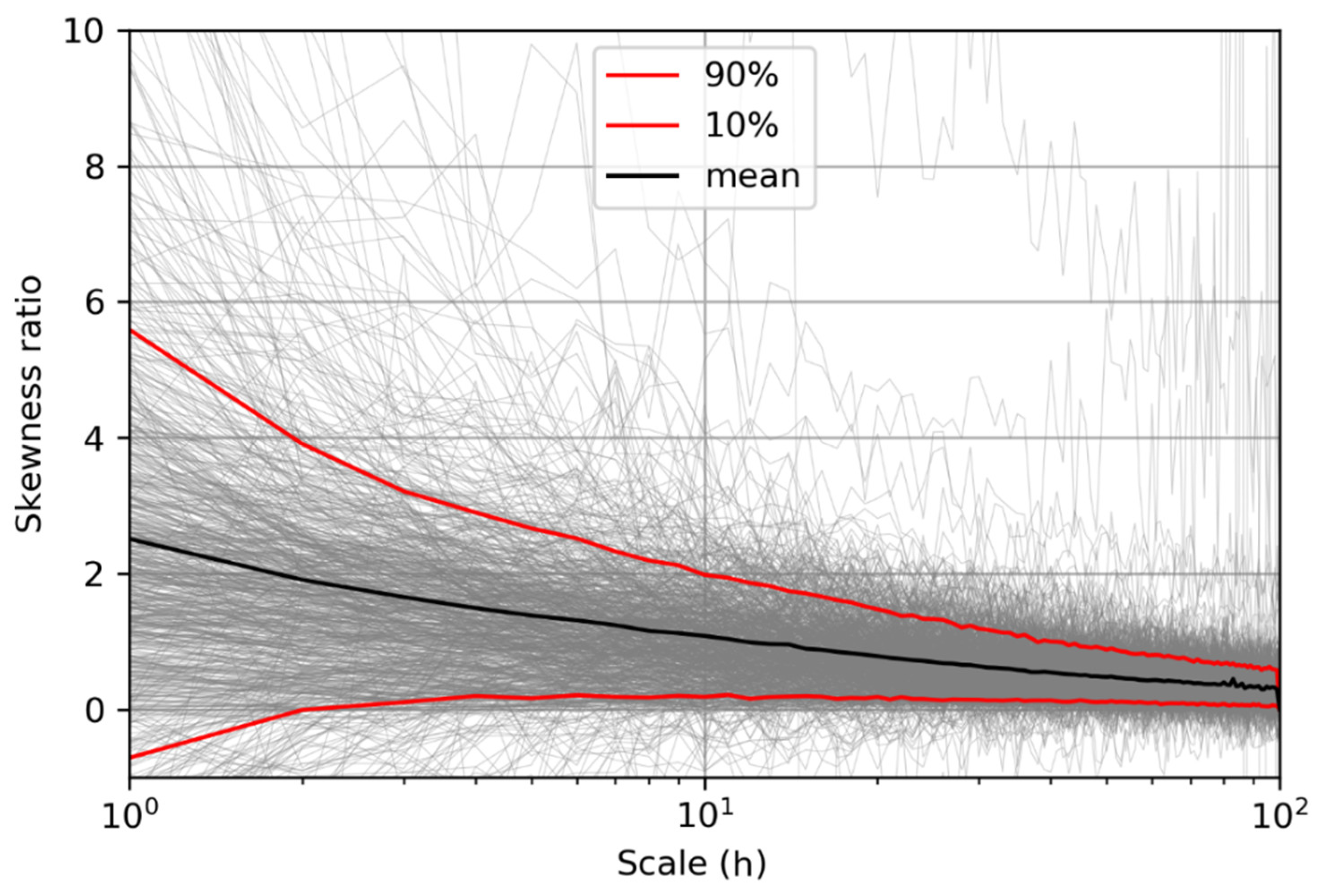
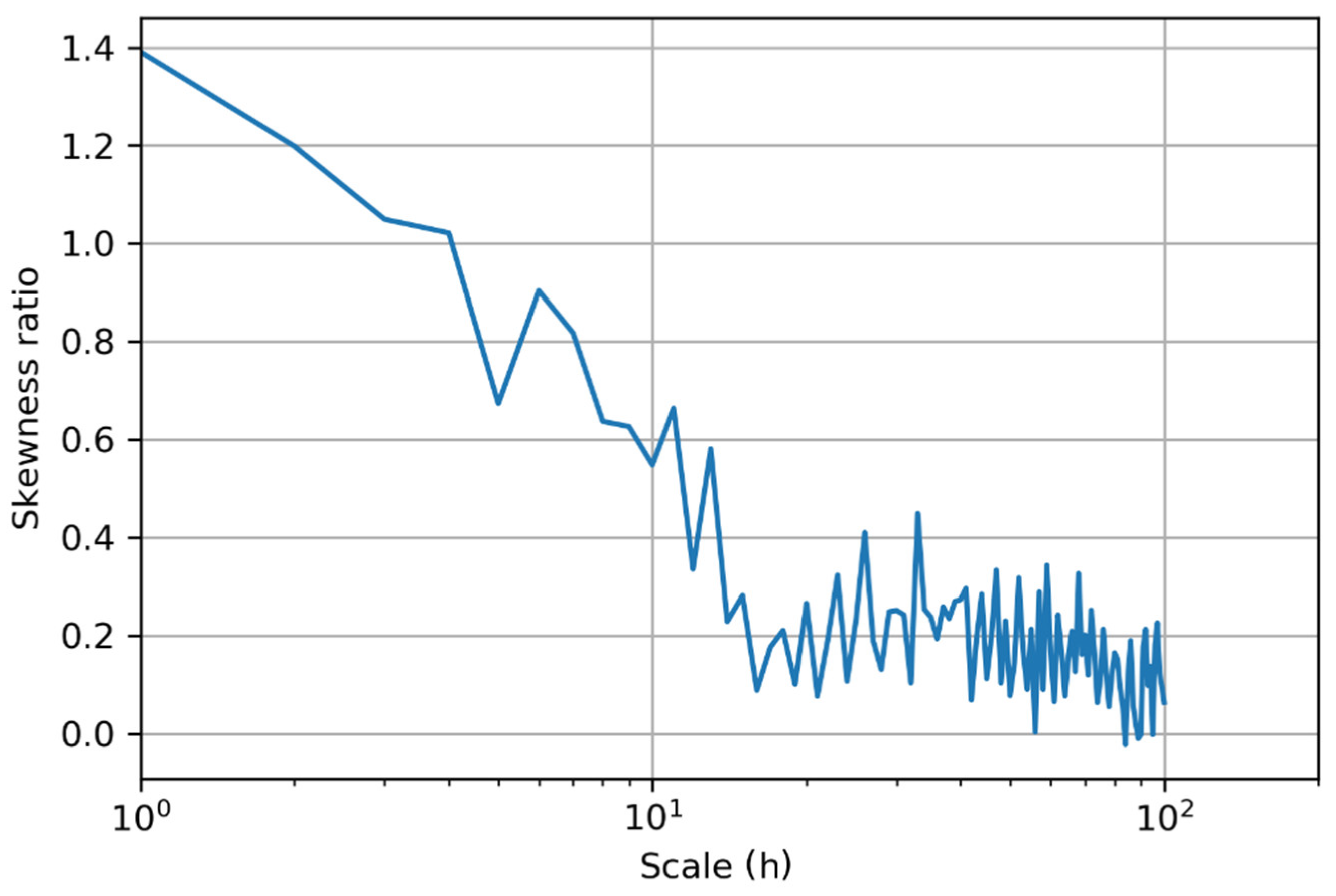
is not symmetric about 0. Our investigation of irreversibility suggests that it is prominent at scales up to the mark of 100 h (i.e., approximately four days) and approaches zero for larger scales. Therefore, it is critical to preserve irreversibility in a wide range of smaller scales. In the current study, the algorithm proposed by Koutsoyiannis [
3,
10], which preserves irreversibility at the basic scale, is modified and extended to simulate time series that preserve the irreversibility at both the first and the second scale. To this aim, it is first important to calculate the theoretical moments of the AMA model at the first and second scale. For a simulation length
the AMA model of Equation (9) can also be expressed as:
where
, with the latter being a lognormal white noise process. Other distributions can be used for even better accuracy [
13]. For the first scale, we must calculate the second and third moments of the differenced and original sequences, respectively. The second moment of the original sequence is:
whereas that of the differenced sequence is:
where we set
, or, more generally, we set
for any
n out of the interval
. The third moment of the original sequence is:
whereas that of the differenced sequence is:
Likewise, for the scale 2 we must calculate the second and third moments of the differenced and original sequences, respectively. We highlight that the process is first averaged at the second scale, according to Equation (5), and afterwards differenced and not the other way around. The second moment of the original sequence at scale 2 can be expressed as:
whereas the second moment of the differenced sequence at scale 2 is:
The third moment of the original sequence at scale 2 is:
whereas the third moment of the differenced sequence at scale 2 is:
After calculating the sample moments, optimization tools are used to estimate the parameters of the AMA model by minimizing the sum of squared errors between the sample (empirical) and the theoretical moments. The parameterization follows the same methodology as in Koutsoyiannis [
10]. The function
is defined as the smooth minimum of two hyperbolic functions
(
of frequency
, i.e.:
where the symbols
and
ζ denote parameters to be determined by optimization.
After the function of
is parameterized, we use it to perform the Fourier transform and express the real part of the result for
. At last, we have the sequence of
, i.e.,:
where
is the imaginary unit,
is an odd real function (meaning
). In turn,
is defined as:
where
represents the power spectrum.
3.3. Stochastic Tools for Multiscale Dependence Characterization
For the characterization of the multiscale dependence, we use the climacogram stochastic metric, which expresses the quantification of change/variability in the scale domain, instead of the common lag (i.e., through the autocovariance or autocorrelation function) and frequency (i.e., through the power-spectrum) domains. The second-order climacogram is defined as the variance of the averaged process
(
t) (Equation (5)) (assumed stationary) versus the averaging time scale
and is symbolized by
[
14]. The climacogram is useful for detecting the long-term change (or else dependence, persistence, clustering) of a process’s multiscale stochastic representation.
The statistical bias in the climacogram estimator can be calculated as follows. As shown in Koutsoyiannis’s study [
15], assuming that we have
observations of the averaged process
, where the observation period
is an integer multiple of
Δ, the time-resolution, the expected value of the empirical (sample) climacogram
is:
The climacogram is also related to the power spectrum and the autocovariance. However, the study by Dimitriadis and Koutsoyiannis [
16] showed that the climacogram had the smallest estimation error among the three tools, while its bias could be computed simply and analytically. Additionally, the fact that its values are always positive is an advantage in stochastic modelling. Moreover, it is well-defined with an intuitive definition and is for the most part monotonic.
Another useful metric in the scale domain is the climacospectrum, which is a newly introduced stochastic tool. It is defined by Koutsoyiannis [
17] as:
where
represents the scale. The asymptotic behaviour of the second-order characteristics of a process for
and
is characterized by two parameters,
and
, which are given by:
where “
” represents the slope on a doubly logarithmic plot (a doubly logarithmic derivative).
The climacospectrum has the following advantages [
17]: In comparison with the power spectrum, it is superior with respect to its connection with the conditional entropy production. Specifically, it is more precise without exceptions. Additionally, the variance, on which the definition of the climacospectrum is based, is more closely related to uncertainty, and as a result to the entropy of the process, than the power spectrum and the autocovariance.
To apply the method to the streamflow series, first the effect of the annual cycle is approximately removed by multiplying the discharge values by 12 different coefficients, one per month, summing up to 1. These coefficients are estimated by minimizing the total variance of the transformed time series.
Then, the Filtered Hurst Kolmogorov model is fitted to the data in order to estimate the parameters
H,
M and
a. The climacogram of the Filtered Hurst Kolmogorov process is given below [
17]:
where
a is a scale parameter, and
M and
H are the fractal and Hurst parameters.
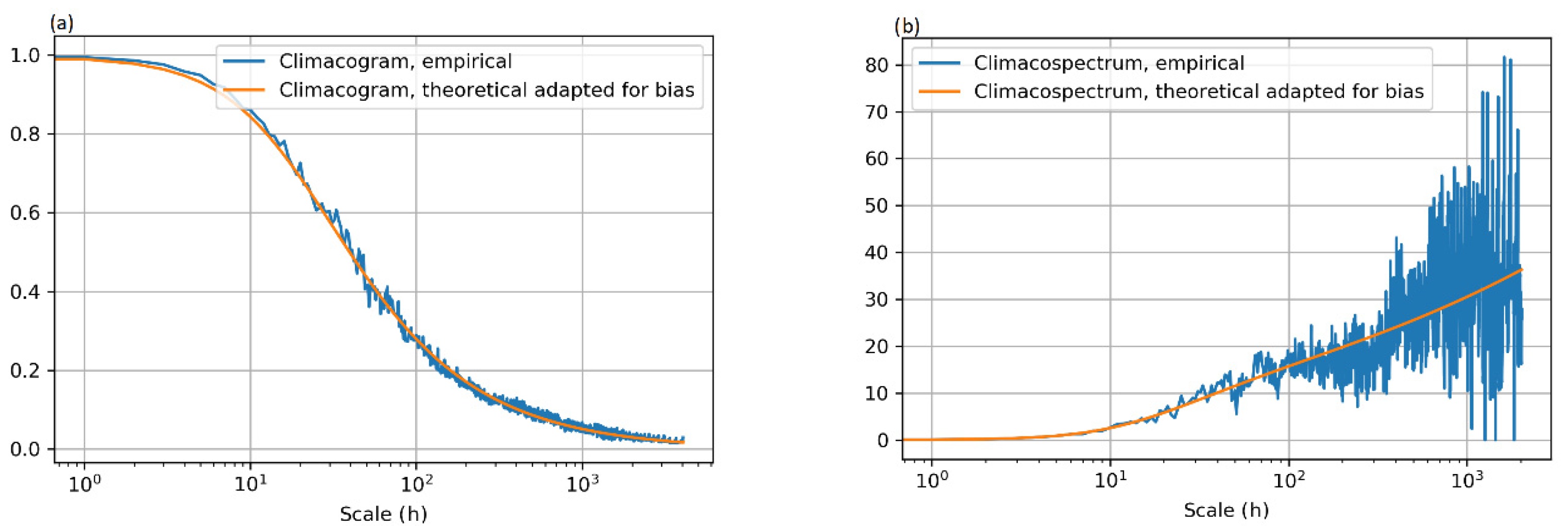
The same calibration function is used for both the climacogram and the climacospectrum (empirical and theoretical), since the climacospectrum is more robust for the analysis of the finer scales and the climacogram is more robust for the analysis of the larger scales. The reason behind this is related to the theoretical context of these stochastic tools, as discussed earlier and in [
16]. We note that both the climacogram and the climacospectrum were adapted for bias.
After that, the discrete power spectrum through the Fast Fourier Transform (FFT) and the AMA coefficient were calculated. The next step was to detect the scale-wise time irreversibility. We aggregate the data up to the 100 h scale and calculate the sample skewness of the differenced and original processes. Their ratio is the irreversibility index, as discussed above. Furthermore, the irreversibility of both scales 1 and 2 was also important to calculate since it was to be preserved later by the algorithm.
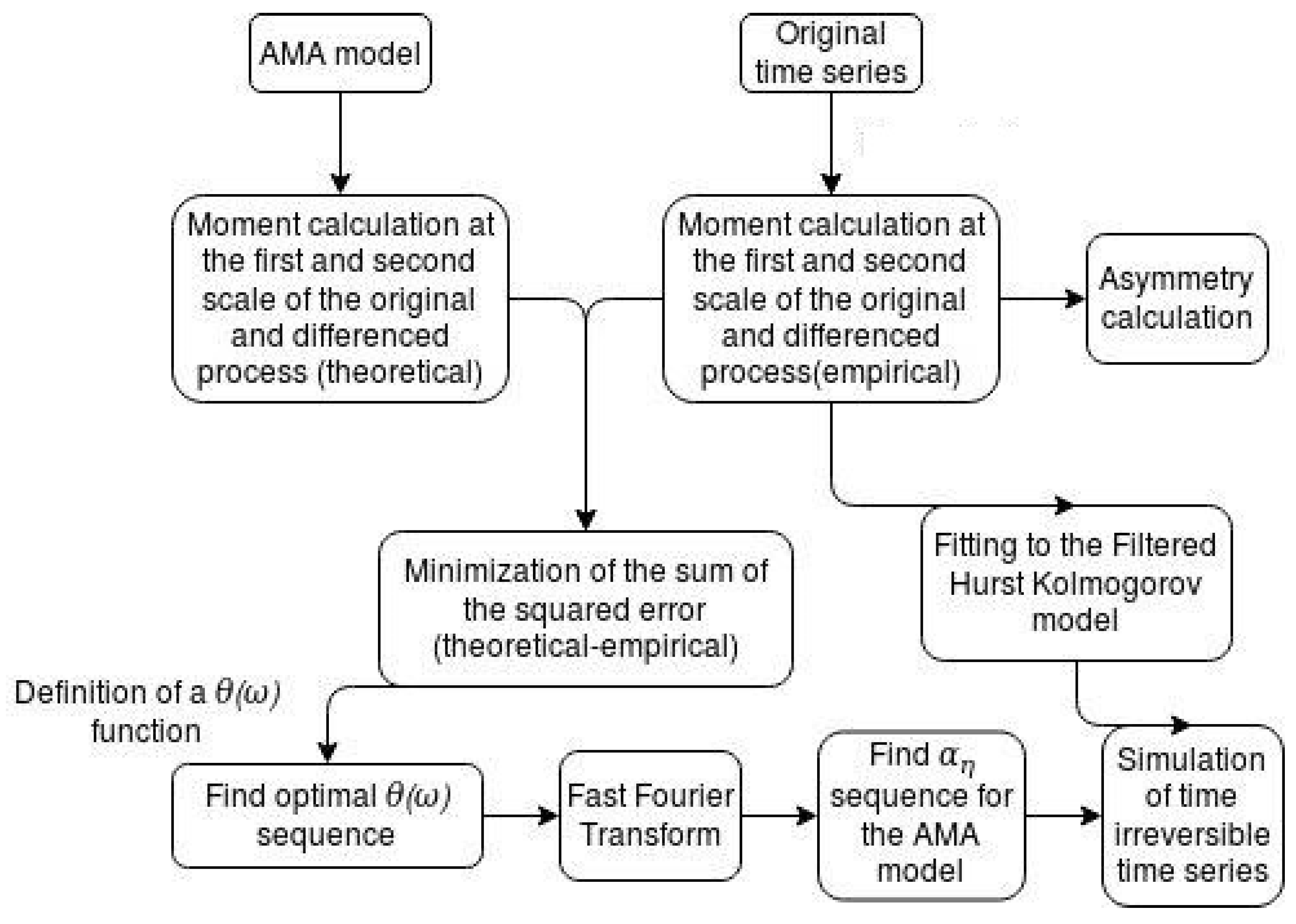
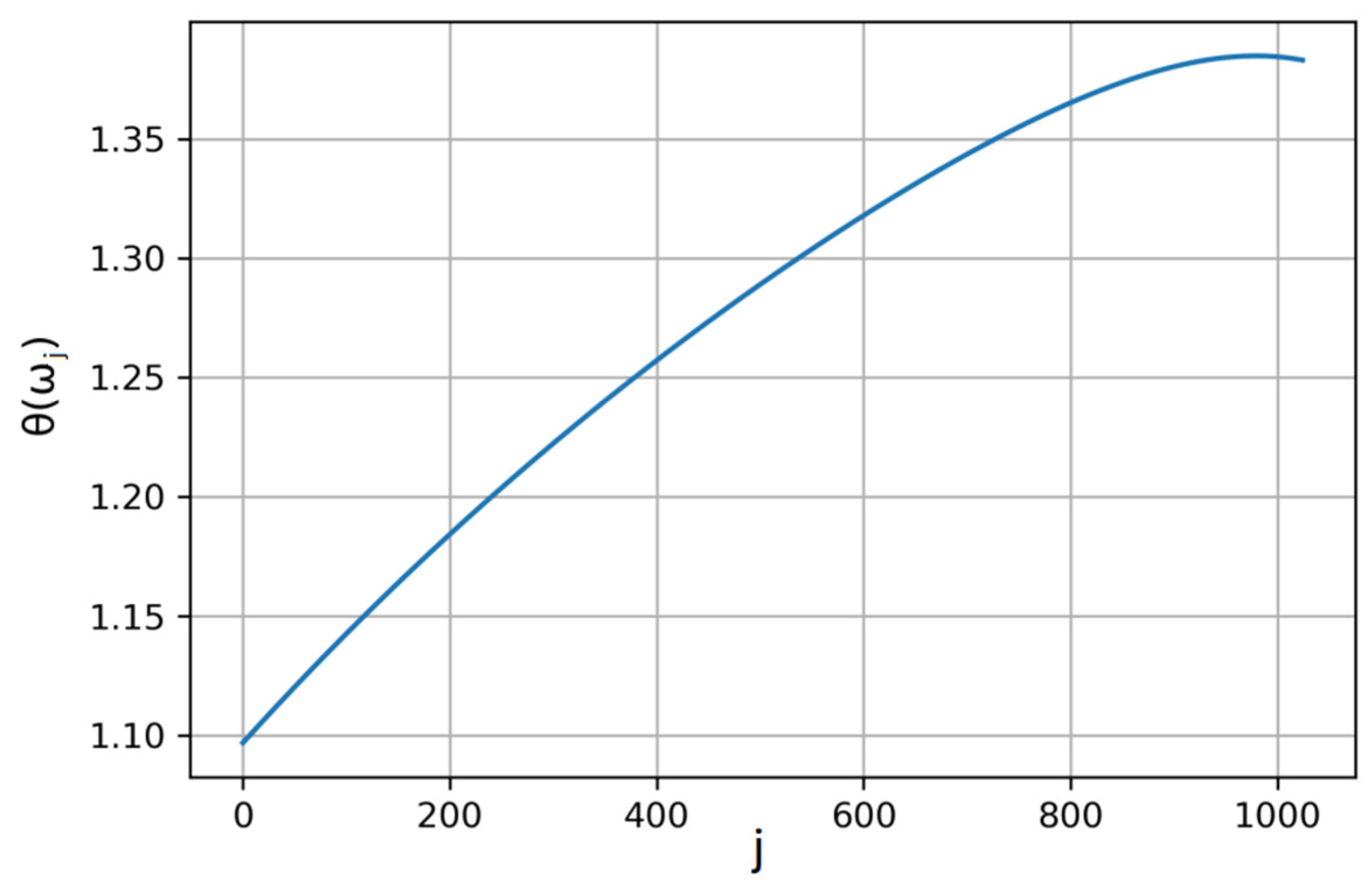
In the first case, i.e., when irreversibility is only preserved at scale one, optimization tools are used to find the parameters needed to estimate the constant θ. In the second case for the sequence θ(ω), which is defined as the smooth minimum of two hyperbolic functions of frequency, optimization was used again. The concept is that after building functions to calculate the sample and theoretical moments, computational tools have to minimize the difference between the sample (empirical) and the theoretical moments. In the second case, the difference is that this happens for two scales and that the square error is minimized. The output is the θ(ω) sequence. With knowledge of the power spectrum and θ(ω) we are able to calculate the AMA coefficients from Equation (20), i.e., the sequence. After this procedure, the synthetic time series can be simulated by applying Equation (9).
Specifically, this methodology generates time series that preserve irreversibility at two timescales along with the second-order dependence properties of the process. For example, if we choose as the basic scale the one-hour scale, the second scale for the irreversibility to be preserved is two hours. In
Figure 1, the complete methodology is shown in steps.
