Effect of Projected Land Use and Climate Change on Water Quality of Old Woman Creek Watershed, Ohio

Abstract

The separate and synergistic effects of land use and climate change on water quality variables in Old Woman Creek (OWC) watershed were evaluated using a hydrological model set up in Soil and Water Assessment Tool (SWAT) for the OWC watershed. Model calibration was done using a multi-objective evolutionary algorithm and pareto optimization. The Parameter-Elevation Regressions on Independent Slopes Model (PRISM) climate data and the 20 different Global Circulation Models (GCMs) developed by the Coupled Model Intercomparison Project Phase five (CMIP5) were used. Validation was done using the streamflow data from USGS gaging station and water quality data from the water quality lab, Heidelberg University. The simulation was divided into two land use scenarios: Scenario 1 for constant land use and Scenario 2 where land use was varied. Both land use simulations were run in four time periods to account for climate change: historical (1985–2014), current to near future (2018–2045), mid-century (2046–2075), and late-century (2076–2100) climate windows. For the historical period, the average of all the simulations made from the 20 different CMIP5 GCMs shows good agreement with the PRISM results for flow and the water quality variables of interest with smaller inter-model variability compared to PRISM results. For the other three climate windows, the results of Scenario 1 show an increase in flow and eight water quality variables (sediment (total suspended sediment), organic nitrogen, organic phosphorus (particulate p), mineral phosphorus (soluble reactive p), chlorophyll a, carbonaceous biochemical oxygen demand (CBOD), dissolved oxygen, total nitrogen) across the climate windows but a slight decrease in one water quality variable, mineral phosphorus in the mid-century. The results of Scenario 2 show a greater increase in flow, and the eight water quality variables across the climate windows show a relatively larger decrease in one water quality variable (mineral phosphorus). The projected land use change has little impact compared to the projected climate change on OWC watershed in the 21st century.

1. Introduction

In previous centuries, the influence of land use/land cover (LULC) changes on water were not recognized. It is now generally acceptable that the analysis of historical effects of LULC can produce knowledge about the present, and inferences about the future [1,2]. LULC are indisputable causes of changes in environmental conditions throughout the world and promote losses in biodiversity and deforestation [3]. The effect of LULC on streamflow has been described in previous studies [4,5]. Gebremicael et al. [6] noted that the conversion of a large area of vegetation into agricultural land in the Blue Nile Basin between 1970 and 2010 increased the wet season flow and decreased the dry season flow. In the upper mid-western United States, the previous land use change reported was the conversion of forest to agricultural land, and the recent land use change was urbanization [7,8]. Niyogi et al. [9] has established that urban growth can significantly affect climate and hydrological balance. Population growth, proximity to major urban centers, and migration pattern can influence urban growth [10,11].

Urban areas have paved or impervious surfaces resulting in reduced infiltration and increased surface runoff into the water bodies [12]. The combined effect of increasing agricultural fertilizers and chemical use and increasing urbanization can severely impact the water quality of a watershed. The synergistic effect of LULC changes and climate changes could further warm the land surface [13]. LULC change and climate change contribute to each other after a long period of time [14,15].

This work attempts to address how the projected 21st century land use and climate change would impact the water quality of OWC watershed. Thus, the goal was to evaluate the separate and the synergistic effects of the projected LULC and climate change in the 21st century on streamflow and nutrient transport in OWC watershed using 20 different Global Circulation Models (GCMs) from the Coupled Model Intercomparison Project Phase five (CMIP5) model ensemble. This involves finding out how close the SWAT simulated flow and water quality variables from the 20 GCMs are with the simulated values from the Parameter-Elevation Regressions on Independent Slopes Model (PRISM) historical climate data (1985–2014). Then, using the predicted LULC and the corresponding GCMs, the flow and water quality variables were simulated for future climate windows up to 2100. The first hypothesis was, if SWAT simulation results from the 20 GCMs are consistent, within error of SWAT simulations run with PRISM data for the historical period, then the 20 GCMs can be used to run simulations for future scenarios. The second hypothesis was that the future projected land use change (−3.6% agriculture and +2.4% in urban) from the present should have an insignificant impact on water quality variables in OWC relative to the projected changes in temperature (+47%) and precipitation (+13%) across the century. The water quality variables of main focus in this study are sediment (total suspended sediment), organic nitrogen, organic phosphorus (particulate p), mineral phosphorus (soluble reactive p), chlorophyll a, carbonaceous biochemical oxygen demand (CBOD), dissolved oxygen, total nitrogen, and total phosphorus.

2. Materials and Methods

2.1. Modeling Scenarios

The analysis was carried out in two scenarios: Scenario 1 where land use is constant and climate is varied, and Scenario 2 where both land use and climate are varied accordingly in four climate windows: W1-historical (1985–2014), W2-current to near future (2018–2045), W3-mid-century (2046–2075), and W4-late-century (2076–2100). For the historical climate window, simulation was set up for 1982–2014, but a warm up period of 3 years was used; hence, the simulation results obtained was from 1985–2014. The following steps were taken to achieve the overall objective:

• PRISM climate data (1985–2014): simulating flow and water quality variables at annual time scale for the historical climate window (1985–2014) using PRISM climate data and the actual land use data.
• CMIP5 GCMs simulation (1985–2014): simulating flow and water quality variables at annual time scale for the historical climate window (1985–2014) using 20 different GCMs climate models and the actual land use data.
• Comparing the simulations made with PRISM with those made with the 20 different GCMs from CMIP5 for the historical climate window (1985–2014).
• Scenario 1 GCMs simulations (2018–2100): simulating flow and water quality variables at annual time scale for the current to near future (2018–2045), mid-century (2046–2075), and late-century (2076–2100) climate windows using 20 GCMs from CMIP5 and constant land use.
• Scenario 2 GCMs simulations (2018–2100): simulating flow and water quality variables at annual time scale for current to near future (2018–2045), mid-century (2046–2075), and late-century (2076–2100) climate windows using 20 GCMs from CMIP5 and the corresponding projected land use data for the climate windows.
• Comparing simulation results for Scenario 1 and Scenario 2.

2.2. Site Description

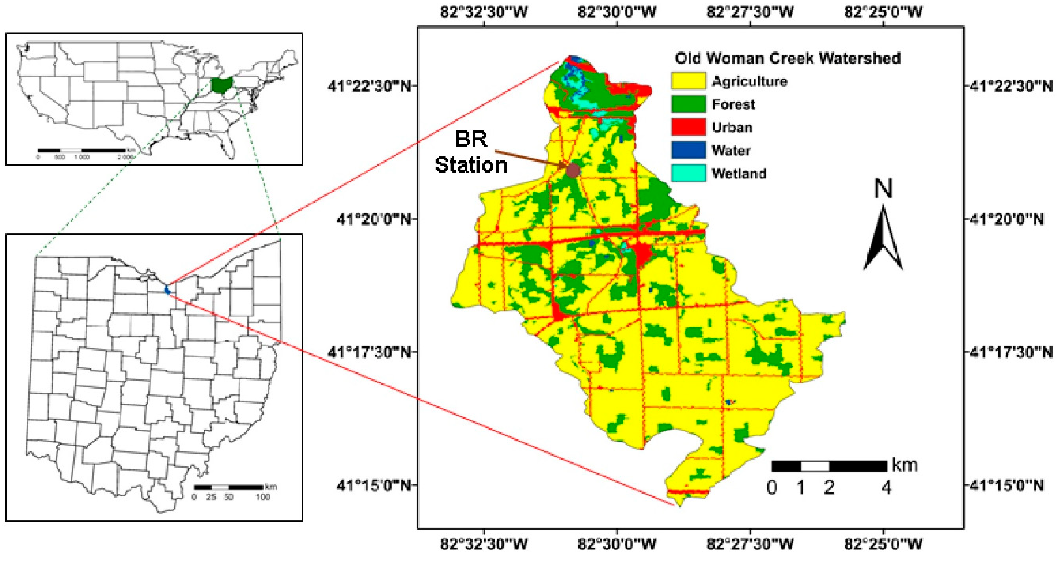
The OWC is located on the south-central shore of Lake Erie in northern Ohio. It drains approximately 69 km² of a watershed mainly used for agriculture [16] (Figure 1) [17]. OWC was selected as a suitable site for the National Estuarine Research Reserve (NERR) System by the National Oceanic and Atmospheric Administration (NOAA) in 1980, and presently, there are only two NERR throughout the Great Lakes regions of North America. In 1995, data loggers were installed at four locations within the estuary for the NERR System-Wide Monitoring Program (SWMP). The Berlin Road (BR) station in the upstream area far south of the estuary was chosen for this research, because it can better measure discharges into the main reservoir, as it is upstream from the effect of hydro-dynamism associated with the mouth of the estuary. Another reason was because of the presence of the USGS gauge station at the BR station where streamflow calibration data were collected.

2.3. Data Acquisition

2.3.1. SWAT Data Acquisition and Preparation

The following data were acquired and used for the hydrological modeling of OWC watershed: OWC shapefile, climate and weather data, digital elevation model (DEM), slope map, land use/land cover map, and digital soil data.

The Ohio state shapefile was obtained from the data catalogue website (https://catalog.data.gov/dataset/tiger-line-shapefile accessed on 22 August 2018) from which the OWC shapefile was extracted to produce all the GIS layers used for this modeling. The 10 m spatial resolution digital elevation model (DEM) of Ohio state was downloaded from national resources conservation services at https://datagateway.nrcs.usda.gov accessed on 31 January 2019. The 30 m resolution LULC data used were downloaded from the National Land Cover Database at https://www.mrlc.gov/data/type/land-cover accessed on 31 January 2019. Digital soil data of Ohio state available at the national resources conservation services website as Soil Survey Geographic (SSURGO) database (https://www.nrcs.usda.gov accessed on 31 January 2021) were used in this work. For the model calibration and validation, the streamflow measurement was obtained from the USGS gauge station at Berlin Road, OWC watershed, Ohio while the water quality data were obtained from the water quality lab, Heidelberg University, Tiffin, Ohio. The SWAT model was run in ArcSWAT GIS interface developed and made available by the Texas A&M University System. The 1981–2017 PRISM climate data with a spatial resolution of 4 × 4 km were downloaded from http://www.PRISM.oregonstate.edu accessed on 31 January 2019. The 1981–2100 CMIP5 model ensemble consisting of the selected 20 GCMs with spatial resolution ranging from Latitude 1.1215 to 2.7906 and Longitude 1.1215 to 3.75 (

Table 1. Original spatial resolution of the 20 Global Circulation Models (GCMs) used in this study (1981–2100).

Institute	Model	GCM_Data	GCMName	Remarks	Latitude	Longitude
CSIRO-BOM	ACCESS1-0	ACCESS1-0	CSIS10	Centre for Australian Weather and Climate Research (CAWCR)	1.25	1.875
CSIRO-BOM	ACCESS1-3	ACCESS1-3	CSIS13	Centre for Australian Weather and Climate Research (CAWCR)	1.25	1.875
BCC	CSM1-1	bcc-csm1-1	BCCSM1	Beijing Climate Center	2.7906	2.8125
BNU	ESM	BNU-ESM	BNUESM	Beijing Normal University	2.7906	2.8125
CCCma	CanESM2	CanESM2	CanESM	Canadian Centre for Climate Modelling and Analysis, Victoria, BC, Canada	2.7906	2.8125
CNRM	CNRM-CM5	CNRM-CM5	CNRCM5	National Centre for Meteorological Research, France	1.4008	1.40625
CSIRO-QCCCE	CSIRO-Mk3-6-0	CSIRO-Mk3-6-0	CSI360	Commonwealth Scientific and Industrial Research Organization/Queensland Climate Change Centre of Excellence (CSIRO-QCCCE)	1.8653	1.875
SMHI	EC-EARTH	EC-EARTH	EEARTH	A European community Earth-System Model, led by SMHI, Sweden	1.1215	1.125
GFDL	CM3	GFDL-CM3	GFDCM3	Geophysical Fluid Dynamics Laboratory, NOAA	2	2.5
GFDL	ESM2G	GFDL-ESM2G	GFDM2G	Geophysical Fluid Dynamics Laboratory, NOAA	2.0225	2.0
GFDL	ESM2M	GFDL-ESM2M	GFDM2M	Geophysical Fluid Dynamics Laboratory, NOAA	2.0225	2.5
MOHC	HadGEM2-CC	HadGEM2-CC	HAD2CC	Met Office Hadley Centre, Hadley Global Environment Model, UK	1.25	1.875
MOHC	HadGEM2-ES	HadGEM2-ES	HAD2ES	Met Office Hadley Centre, Hadley Global Environment Model, UK	1.25	1.875
INM	CM4	INMCM4	INMCM4	Russian Institute for Numerical Mathematics Climate Model Version 4	1.5	2
IPSL	CM5A-LR	IPSL-CM5A-LR	IPSALR	Institut Pierre Simon Laplace, France	1.8947	3.75
IPSL	CM5A-MR	IPSL-CM5A-MR	IPSAMR	Institut Pierre Simon Laplace, France	1.2676	2.5
IPSL	IPSL-CM5B-LR	IPSL-CM5B-LR	IPSBLR	Institut Pierre Simon Laplace, France	1.8947	3.75
MPI	ESM-LR	MPI-ESM-LR	MPIMLR	Max Planck Institute, Germany	1.8653	1.875
MPI	MPI-ESM-MR	MPI-ESM-MR	MPIMMR	Max Planck Institute, Germany	1.8653	1.875
NCC	NorESM1-M	NorESM1-M	NORM1M	Norwegian Climate Centre Earth System Model M	1.8947	2.5

) was downloaded from the climate data store (CDS) catalogue, downscaled to 4 × 4 km resolution, and bias-corrected using the distribution-based scaling (DBS) method described by Yang et al. [18]. The 20 GCMs from CMIP5 at RCP 8.5 only were selected for the analysis to test the performance of each model and identify the most suitable GCM models for the OWC watershed simulation. The 20 GCMs selected consist of 19 GCMs available at the global users in the Copernicus climate change service (C3S_422_Lot1_SMHI project) and one North American GCM (CAN-ESM2). The calibration and validation data were available from 2015–2017, and hence, the future climate window for this study starts from 2018.

2.3.2. SWAT Model

The widely used Soil and Water Assessment Tool (SWAT) is a watershed based hydrological modeling framework produced by Jeff Arnold by upgrading the Simulator for Water in Rural Basins (SWRRB). It was primarily produced for the United States Department of Agriculture, Agricultural Research Services (USDA-ARS) to appraise the influence of environmental pollution and land management practices on water quality. It can simulate the effect of management practices on streamflow and water quality within a large basin with dynamic soil and management practices for a long-time frame [19].

SWAT is capable of efficient simulation on a daily, monthly, and yearly time scale using spatial and meteorological data as input. Arnold et al. [20] gave a detailed account of SWAT parameters and units, some of which include weather, crop yield, soil types, fertilizer application, and hydrological processes. In SWAT modeling, the whole basin is divided into reaches that are further divided into the smallest units called the hydrological response units (HRU). The spatial data needed for hydrological modeling are uploaded into SWAT through the ArcSWAT 2012 graphical interface [21,22].

2.3.3. Model Set-Up, Calibration, and Validation

The ArcSWAT 2012 was employed for the setting up of SWAT for hydrological models. To prepare the model for watershed delineation, drainage, and slope definition, OWC watershed DEM was loaded, and digital stream data added to establish the stream network. The SWAT inbuilt minimum threshold approach based on the minimum area function was used to automatically generate the outlets for the sub-basins, and other outlets were manually added at important locations including one outlet leading to the location of the USGS gauge station (Berlin Road) where calibration and validation data were obtained. OWC watershed was delineated with a size of 66.95 km² and a total of 103 sub-basins. Sub-basins characterization involves the creation of 3 slope classes, which include 3, 3–15, and >15%, and 12 land use classes, which include barren land, open waters, developed high intensity, developed low intensity, developed open space, developed medium intensity, hay/pasture, woody wetlands, evergreen forest, cultivated crops, herbaceous and deciduous forest, and 81 soil classes (Based on SSURGO classification). Land use, slope, and soil were reclassified, and 479 HRUs were created to complete the HRU definition process. SWAT editor was used to encode management practices for the different crops (corn, soya, and wheat) planted in the watershed based on the actual conditions on agricultural land in OWC watershed. The management practices include crop rotation, tillage, fertilizer application, planting time, and harvesting time.

PRISM temperature (min, max, and daily average) and precipitation (1981–2017) were added to the setup, other climate parameters including wind speed, solar radiation, and relative humidity were generated by SWAT for the modeling. The sensitivity of the SWAT parameters to water quality variables was ascertained, and a total of the 56 most sensitive parameters were selected for calibration.

The selected parameters were optimized by modifying the multi-objective evolutionary algorithm method developed by Confesor and Whittaker [23]. The curve number for each of the 479 HRU was calibrated separately, and the soil evaporation compensation factor for each of the 12 land use groups was calibrated separately. The limits of the parameters to be optimized were fixed based on the results obtained from sensitivity analysis. The USGS gauging station at Berlin Road offers the most consistent daily streamflow measurement record between 2015 and 2017, and thus, the model calibration period was set to 5 May 2005–31 December 2016 (607 observations) and the validation period set to 1 January–31 December 2017 (365 observations). A warm-up period of 3 years was used in all simulations. The calibrated and validated variables are streamflow, sediment (TSS), organic nitrogen, mineral phosphorus (SRP), organic phosphorus, total nitrogen, and total phosphorus. Three water quality variables including chlorophyll a, CBOD, and dissolved oxygen were not calibrated because of lack of data, and this may impact the results reported for these three variables.

The generic algorithm package (genalg) in R statistical language [24] was modified and used to randomly create the first 1000 solutions of the parent population from which the 1000 solutions of the child population were generated using five objective functions (flow, TSS, total p, SRP, and total n). The calibration parameters were modified on the fly, and SWAT was run as an R subroutine for each of the solutions and the iteration was stopped at 200. A total of 201,000 SWAT runs were made with 200 iterations.

2.3.4. Objective Function and Model Performance Evaluation

The five objective functions (flow, TSS, total p, SRP, and total n) were used to keep the average root mean square error (RMSE) of the observed versus simulated at minimum. The RMSE equation is given as:

$$RMSE = {\left.\left(\frac{1}{n}{\displaystyle \sum }_{i=1}^n{\left(Q_{sm,i}-Q_{ob,i}\right)}^2\right.\right)}^{0.5}$$

(1)

The performance of the calibrated SWAT model was evaluated by comparing the simulated with the observed variables using three statistical indices: percentage bias/percentage error (P_BIAS (%)), Nash–Sutcliffe model efficiency (NSE) [25] and coefficient of R².

$$PBIAS\left[\%\right]=\frac{{\sum }_{i=1}^n\left(ob-sm\right)\times 100}{{\sum }_{i=1}^{n}ob}$$

(2)

$$NSE=1-\frac{\frac{1}{n}{\sum }_{i=1}^n{\left(Q_{sm,i}-Q_{ob,i}\right)}^2}{\frac{1}{n}{\sum }_{i=1}^n{\left(Q_{sm,i}-Q_{\overline{ob},i}\right)}^2}$$

(3)

$${\mathrm{R}}^2=\frac{{\left[\left({\sum }_{i=1}^n\left(ob-\overline{ob}\right)\right)\left(sm-\overline{sm}\right)\right]}^2}{{\sum }_{i=1}^n{\left(ob-\overline{ob}\right)}^2{\sum }_{i=1}^n{\left(sm-\overline{sm}\right)}^2}$$

(4)

where Q_Ob and Q_Sm are the observed (measured) and the simulated daily streamflow at a given time i, and n represents the total number of observations for the simulation.

NSE ranges from negative infinity to 1, with 1 indicating a perfect match between the observed and simulated.

2.4. Scenario Simulations

A total of 141 annual simulations were made in this work to analyze the response of 10 water quality variables. For the historical (first) climate window (1985–2014), a total of 21 simulations were made. Only one simulation was run with PRISM climate data, 20 simulations were run with 20 GCMs, and the results were compared to establish the extent to which CMIP5 GCMs can reproduce the actual (PRISM climate) results. For the Scenario 1 of the current to near future (2018–2045), mid-century (2046–2075), and late-century (2076–2100) climate windows, a total of 60 simulations were made using 20 GCMs in each climate window with constant (current) LULC data applied across all the climate windows. For Scenario 2 of the current to near future (2018–2045), mid-century (2046–2075), and late-century (2076–2100) climate windows, a total of 60 simulations were also made using 20 GCMs in each climate window with the respective projected LULC applied for each climate window, and the results of the two scenarios were compared.

3. Results

3.1. Historical (PRISM) and Projected (CMIP5) Climate Forcing

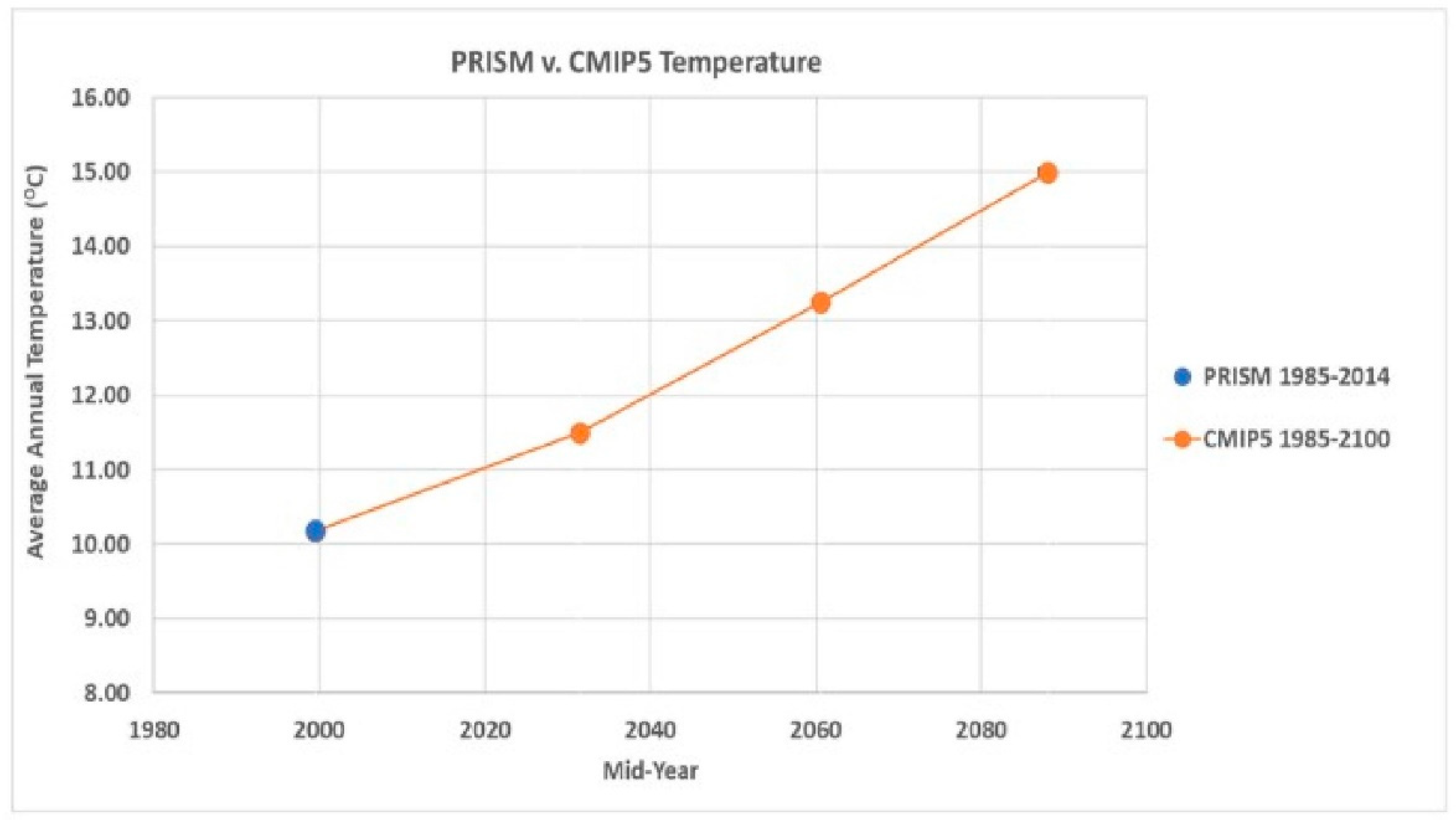
The PRISM and GCMs climate forcing used for the simulations of flow and water quality variables in OWC watershed for the 21st century are shown in Figure 2 and Figure 3. For the historical climate window, PRISM results were averaged to remove inter-annual variability within the climate window. For each of the four climate windows, the results of the simulations made from the 20 different GCMs were first averaged across the model to remove inter model variability, and the results averaged to remove inter annual variability within the climate window. Comparison of precipitation data in the historical climate window shows that GCMs slightly underestimated precipitation with an annual average value of 937.7 mm compared to the actual (PRISM climate) with an annual average value of 962.4 mm, but the underestimation is statistically insignificant as the error bar from GCMs’ results overlaps PRISM result. The GCMs’ precipitation increases almost linearly from 937.7 mm in the historical climate window to 1060.7 mm in the late-century climate window. The percentage increase in average annual precipitation relative to the historical climate window for the current–future, mid-century, and late-century climate windows are 4.2, 7.6, and 13.1% respectively.

For the historical climate window, PRISM and CMIP5 GCMs temperatures are almost the same with values of 10.19 and 10.18 °C, respectively. CMIP5 GCMs’ temperature increases almost linearly from the historical climate window with an annual average of 10.18 °C to the last climate window with an annual average of 14.99 °C. The percentage increase in average annual temperature relative to the historical climate window for the current–future, mid-century, and late-century climate windows are 12.9, 30.1, and 47.3% respectively.

The error bars were constructed from the standard deviation of the projected climate data and show the degree of variability in each data. The variability observed between the average of the 20 GCMs’ result and the PRISM data is statistically insignificant as shown by the overlapping error bars (Figure 2 and Figure 3). In short, the average of 20 GCMs is consistent with the PRISM climate data for the OWC watershed and can be used to run simulations for the future scenarios.

3.2. Land Use Forcing

The OWC watershed is primarily agricultural, and the LULC has not been changing significantly over the past years. The land use forcing in this analysis is shown in

Table 2. Land use/land cover (LULC) forcing used in the simulation.

Climate Window	Mid-Year	Agriculture (%)	Forest (%)	Urban (%)	Water (%)	Wetland (%)
PRISM 1985–2014	1999.5	65.42	25.14	8.12	0.50	0.82
20 CMIP5 GCMs 1985–2014	1999.5	65.42	25.14	8.12	0.50	0.82
20 CMIP5 GCMs Scenario 1_2018–2100	2031.5	65.18	24.95	8.44	0.62	0.81
20 CMIP5 GCMs Scenario 2_2018-45	2031.5	64.38	25.02	9.02	0.73	0.84
20 CMIP5 GCMs Scenario 2_2046-75	2060.5	63.16	25.30	9.96	0.73	0.84
20 CMIP5 GCMs Scenario 2_2076-00	2088	61.58	26.01	10.82	0.73	0.85

, and it represents the average over the climate window. The land use data averaged over the period 1985–2014 were used for the simulations in the historical climate window. For Scenario 1, the baseline calibration land use data, which represents the average of 2015–2017, was used as a constant land use data for simulations for all climate windows. For Scenario 2, the projected land use data, generated using joint MLP-CA Markov model and averaged over the respective climate window, were used for all the simulations. The agricultural land in the OWC watershed is projected to decrease across the century, while urbanization is projected to increase slightly across the century (Table 2 and

Table 3. Percentages change in forcing from the historical climate window.

Forcing	(W2–W1) %	(W3–W1) %	(W4–W1) %
Precipitation	4.2	7.6	13.1
Temperature	12.9	30.1	47.3
Agriculture	−1.04	−2.26	−3.84
Urbanization	0.9	1.84	2.7

).

3.3. PRISM and CMIP5 GCMs Inter-Model Variability Results (1985–2014)

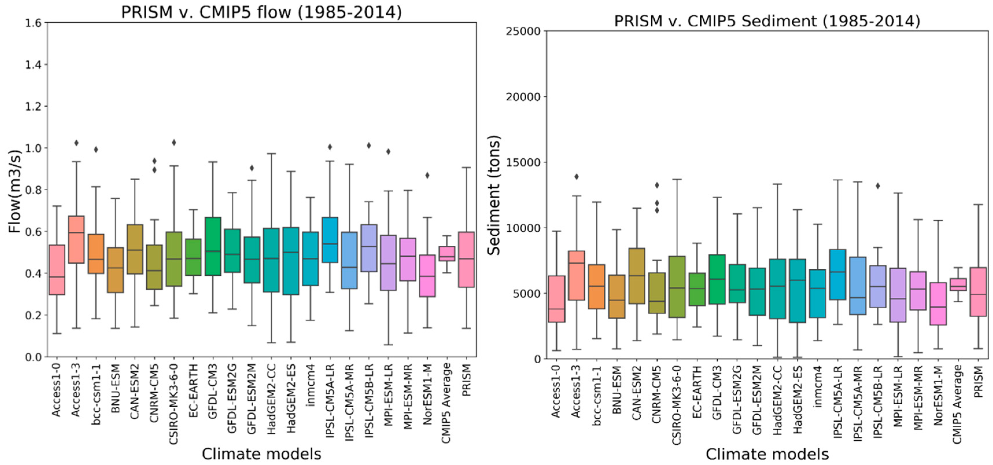
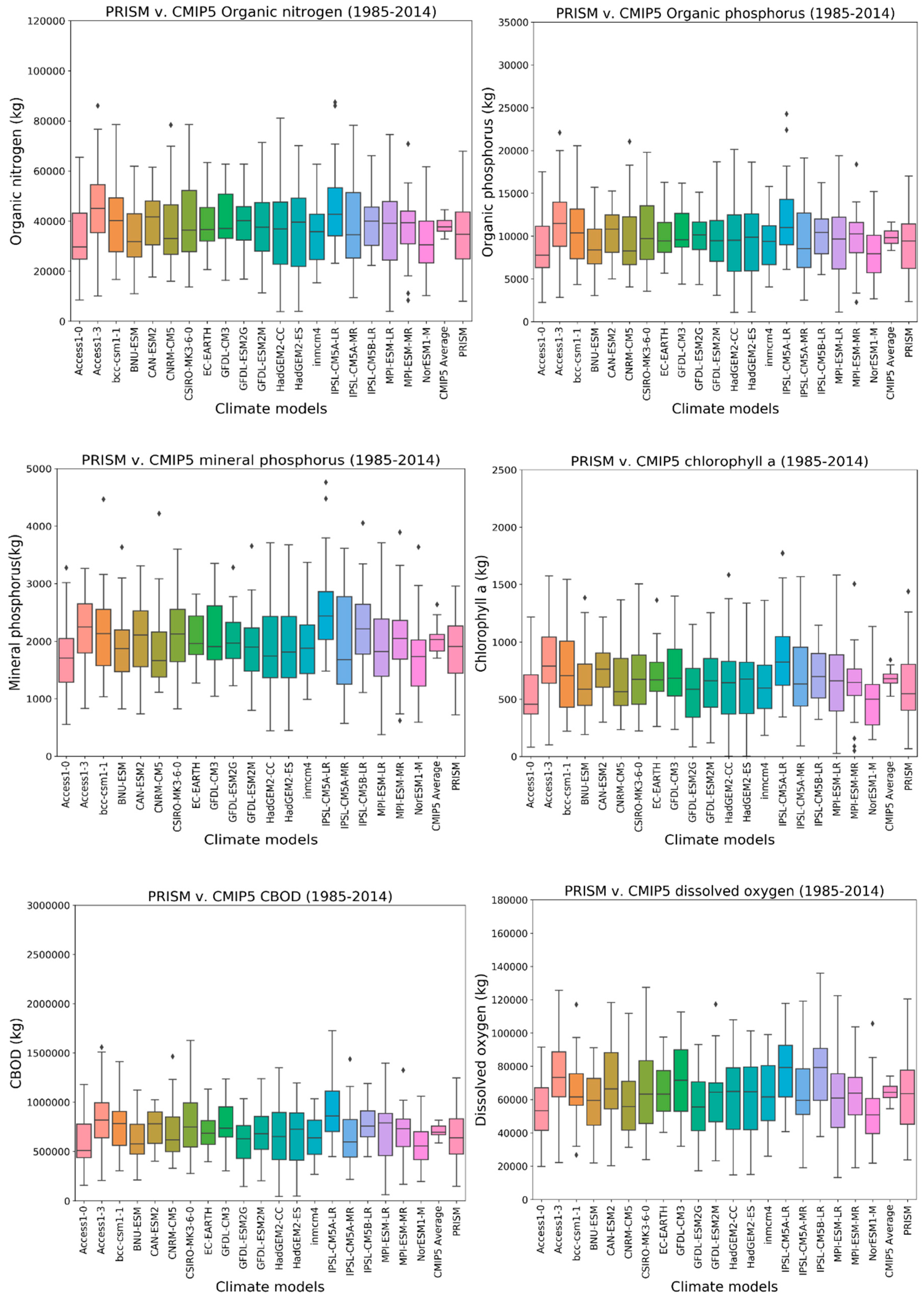
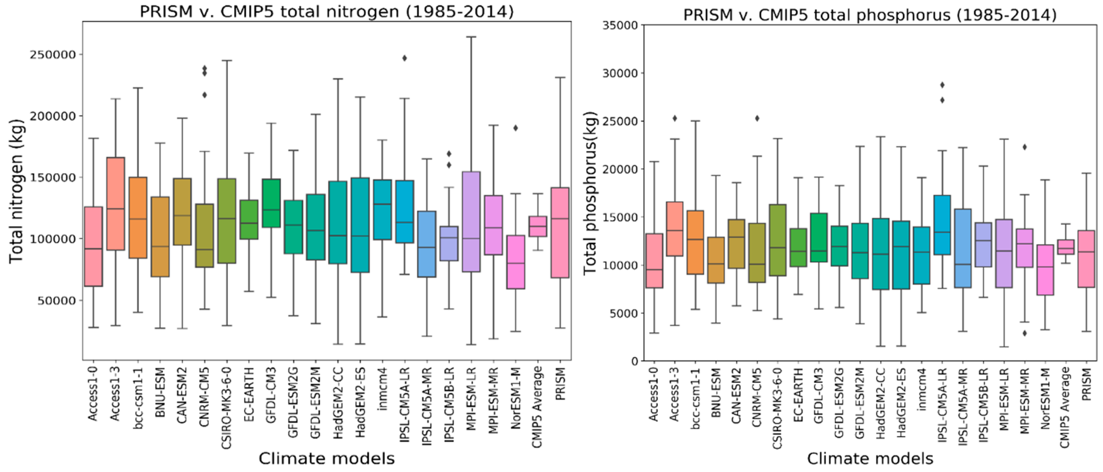
The results of the simulations made with PRISM and the 20 GCMs for flow and nine water quality variables are shown in boxplots in the Appendix A, while the summary of the statistics of the boxplots and the mean are shown in

Table 4. Flow and WQ comparison between PRISM and average of 20 CMIP5 GCMs (1985–2014).

	Streamflow (m3/s)		Sediment (tons)		Organic Nitrogen (kg)		Organic Phosphorus (kg)		Mineral Phosphorus (kg)
	CMIP5 Avg.	PRISM	CMIP5 Avg.	PRISM	CMIP5 Avg.	PRISM	CMIP5 Avg.	PRISM	CMIP5 Avg.	PRISM
mean	0.49	0.46	5612	5022	38,508	35,955	9949	9353	2020	1848
std	0.04	0.19	659	2744	3350	16,130	947	4053	225	616
min	0.40	0.14	4362	783	32,802	8060	8318	2344	1705	722
0.25	0.46	0.33	5210	3250	35,908	24,908	9149	6230	1829	1442
0.50	0.48	0.47	5530	4919	37,731	34,775	9796	9422	2030	1910
0.75	0.53	0.60	6114	6948	40,318	43,675	10,621	11,409	2120	2264
max	0.58	0.91	6944	11,754	44,516	67,890	11,638	16,998	2639	2953
Outliers	NA	NA	NA	NA	NA	NA	NA	NA	2639.40	NA
	Chlorophyll a (kg)		CBOD (kg)		Dissolved Oxygen (kg)		Total Nitrogen (kg)		Total Phosphorus (kg)
	CMIP5 Avg.	PRISM	CMIP5 Avg.	PRISM	CMIP5 Avg.	PRISM	CMIP5 Avg.	PRISM	CMIP5 Avg.	PRISM
mean	685	614	711,384	676,462	64,550	63,389	111,316	107,745	11,969	11,201
std	66	363	59,993	298,464	4661	22,825	11,479	45,366	1091	4630
min	526	68	585,142	150,120	54,488	23,734	90,422	27,490	10,163	3066
0.25	640	404	670,726	473,875	61,231	45,250	101,697	68,085	11,141	7682
0.5	679	548	695,898	639,800	64,287	63,510	110,149	116,150	11,719	11,359
0.75	720	805	759,646	830,975	68,018	77740	118,118	141,418	12,629	13,590
max	843	1440	816,880	1,247,400	74,023	120,440	136,440	231,150	14,278	19,558
Outliers	843	1440	NA	NA	NA	NA	NA	NA	NA	NA

CBOD = carbonaceous biochemical oxygen demand.

. Each of the 20 GCMs’ results and the average of the 20 GCMs’ results was compared with the PRISM result, and it was found that the results of each of the 20 GCMs shows different variability with PRISM result across all variables but the average of the 20 GCMs’ results is more consistent with the PRISM result across all variables when compared along the mean and median values. For all the water quality variables studied, the average of the 20 GCMs’ results slightly and consistently overestimated the 10 variables of interest within the error of SWAT simulations. The variability observed in the average of 20 GCMs’ results is smaller than that of the PRISM result. This is because the GCMs’ results represent the average of 20 models, while the PRISM result is one model result. In Table 4, the mean and median values for the average of 20 GCMs (0.49, 0.48 m³/s) and PRISM (0.46, 0.47 m³/s) for flow are consistent. For sediment, the mean and the median values for the average of 20 GCMs (5612, 5530 tons) and PRISM (5022, 4919 tons) are also consistent. For all the 10 variables of interest, the mean of the average of the 20 GCMs’ results is slightly and consistently higher than that of the PRISM results.

3.4. Scenario 1 and Scenario 2 CMIP5 Inter-Model Variability Results (2018–2100)

The statistics of the boxplots and the mean for the simulation results for the 10 variables of interest for Scenario 1 and Scenario 2 in the current–future climate windows are presented in

Table 5. Comparison between Scenario 1 and 2 (2018–2045).

	Streamflow (m3/s)		Sediment (tons)		Organic Nitrogen (kg)		Organic Phosphorus (kg)		Mineral Phosphorus (kg)
	Scen01	Scen02	Scen01	Scen02	Scen01	Scen02	Scen01	Scen02	Scen01	Scen02
mean	0.52	0.53	6235	6333	40,002	40,409	10,162	10,426	2000	1784
std	0.05	0.05	717	706	4012	4332	1002	1222	260	181
min	0.43	0.44	4717	4935	31,333	30,921	7918	7811	1512	1383
0.25	0.49	0.50	5769	5821	37,410	38,315	9608	9671	1782	1703
0.50	0.52	0.52	6215	6249	39,761	40,217	10,056	10,330	1984	1799
0.75	0.55	0.56	6669	6798	42,306	42,776	10,731	11,061	2206	1871
max	0.62	0.63	7608	7888	47,797	49,009	12,406	12,807	2455	2184
Outliers	NA	NA	NA	NA	NA	30,921	7918	NA	NA	1383
Outliers	NA	NA	NA	NA	NA	NA	NA	NA	NA	2184
	Chlorophyll a (kg)		CBOD (kg)		Dissolved Oxygen (kg)		Total Nitrogen (kg)		Total Phosphorus (kg)
	Scen01	Scen02	Scen01	Scen02	Scen01	Scen02	Scen01	Scen02	Scen01	Scen02
mean	729	740	789,545	800,144	69,059	70,383	113,825	115,888	12,161	12,210
std	86	93	76,029	83,016	5541	5442	8561	9809	1180	1385
min	539	545	634,984	639,485	57,923	60,339	92,602	95,596	9430	9193
0.25	684	694	734,296	739,323	65,354	65,988	108,870	111,399	11,508	11,415
0.5	728	744	787,588	800,900	68,558	69,894	114,154	116,270	12,106	12,100
0.75	769	785	831,460	845,954	72,442	73,579	118,622	120,835	12,808	12,997
max	888	933	940,055	972,310	81,836	83,041	131,080	132,349	14,566	14,821
Outliers	557	545	NA	NA	NA	NA	92,602	95,596	9430	NA
Outliers	538.83	933.25	NA	NA	NA	NA	NA	NA	NA	NA

. It should be noted that the simulated results for the water quality variables reflect the synergistic effect of flow, other mechanisms of nutrients generation within the system, and model uncertainty, which is not separable. In this study, emphasis is placed on the respected effects of the main model forcing (climate change and LULC) over other mechanisms. The results reveal slight differences between Scenario 1 and 2. 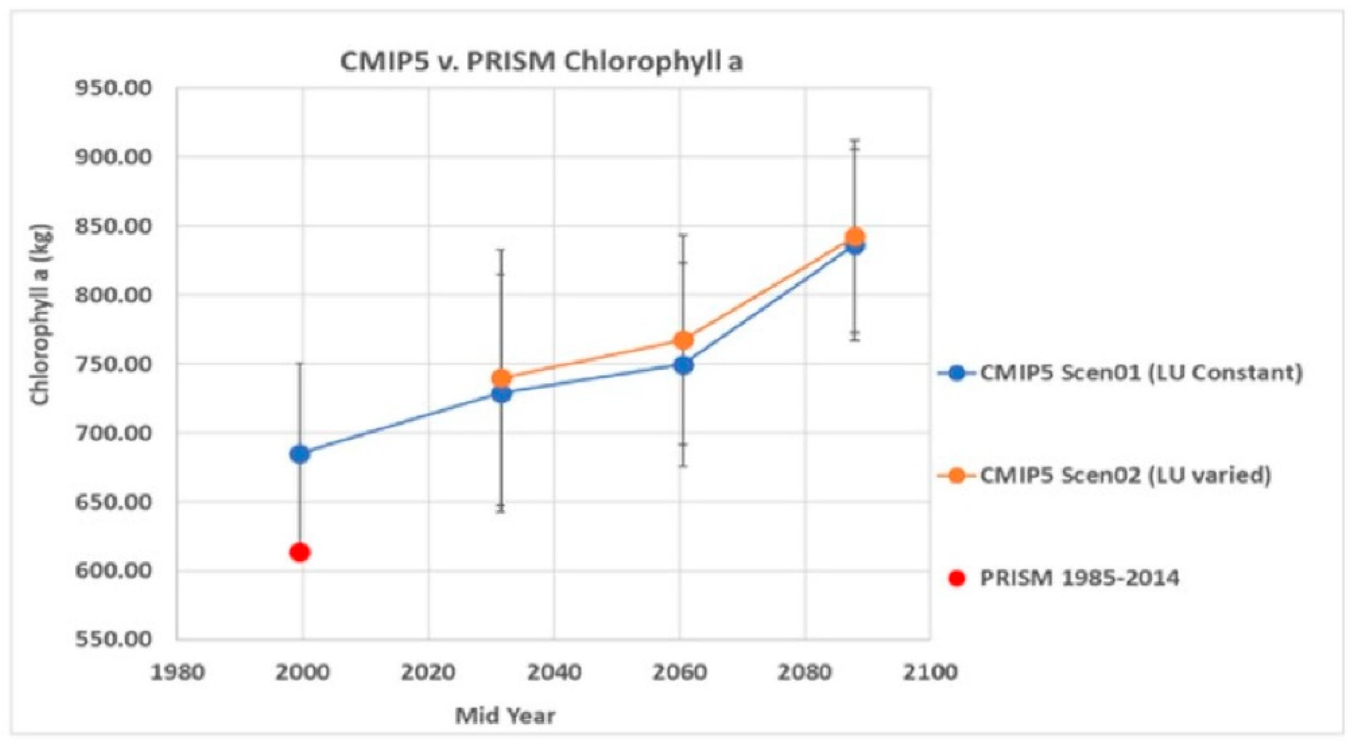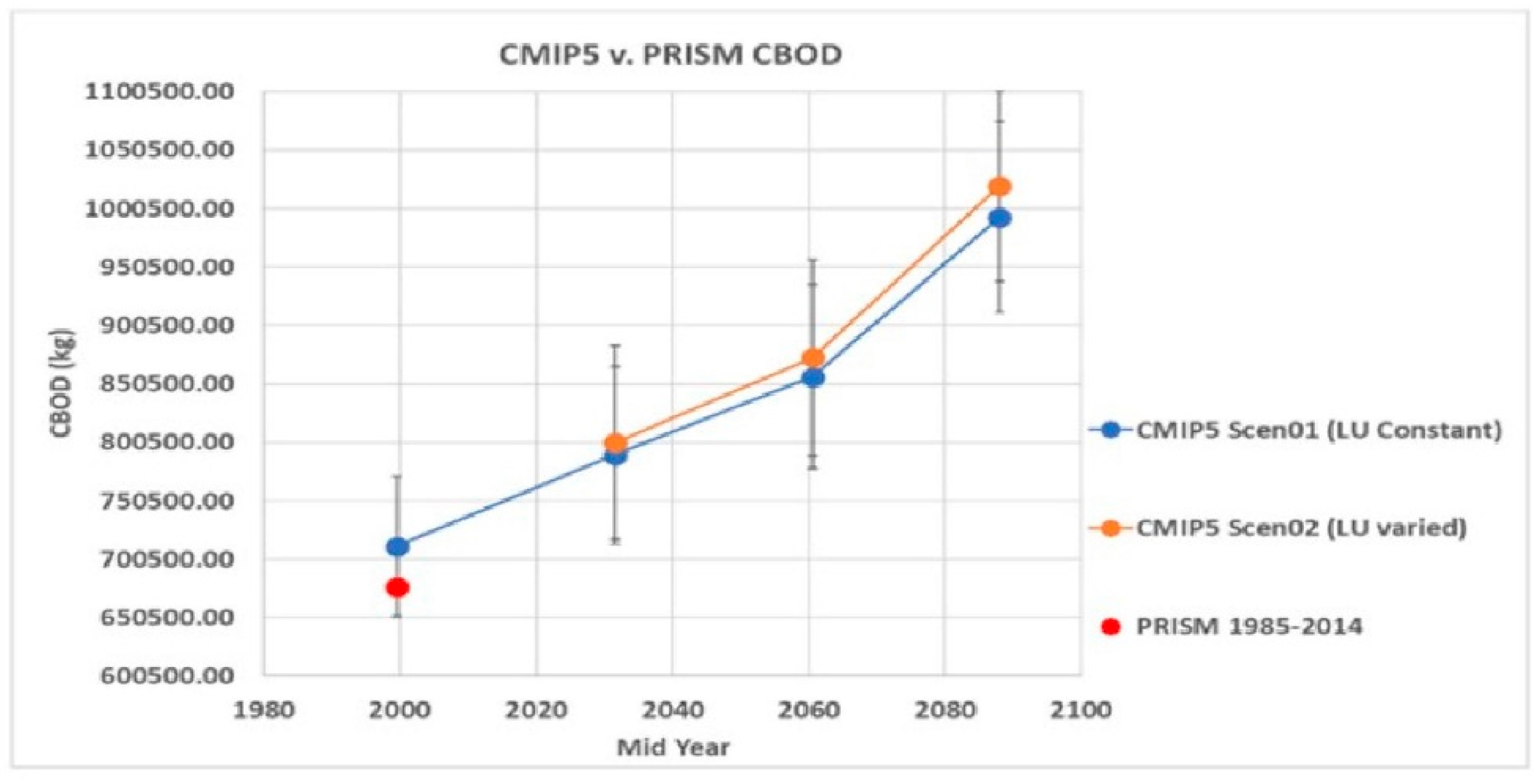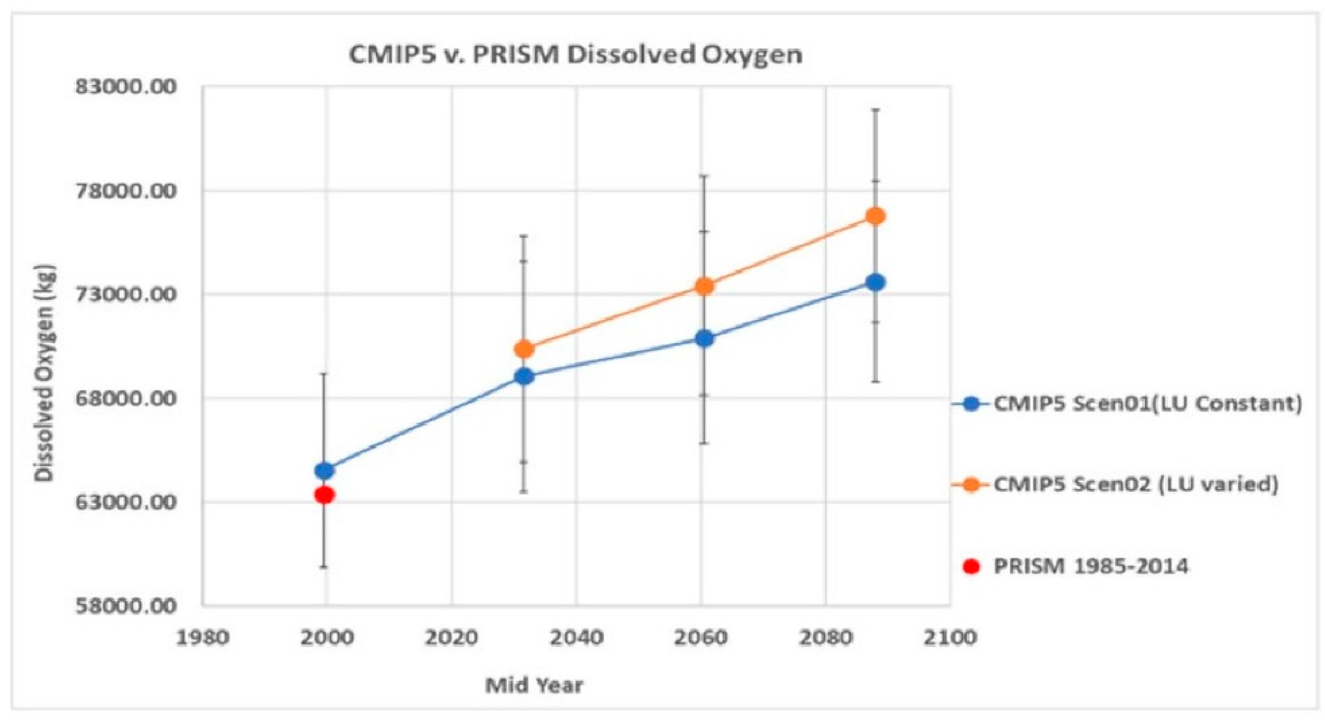The mean, median, minimum, and maximum values for streamflow in Scenario 1 are 0.52, 0.52, 0.43, and 0.62 m³/s, respectively, and in Scenario 2 are 0.53, 0.52, 0.44, and 0.63 m³/s, respectively. The slight increase in streamflow in Scenario 2 is attributed to a small decrease (0.8%) in agriculture and 0.58% increase in urbanization in relation to Scenario 1. The mean sediment transport for Scenario 1 and Scenario 2 are 6235 and 6333 tons, median values are 6215 and 6249 tons, minimum values are 4717 and 4935 tons, and the maximum values are 7608 and 7888 tons, respectively. Similar trends were observed for organic nitrogen transport, organic phosphorus, chlorophyll a, CBOD, dissolved oxygen, total nitrogen, and total phosphorus, and precipitation

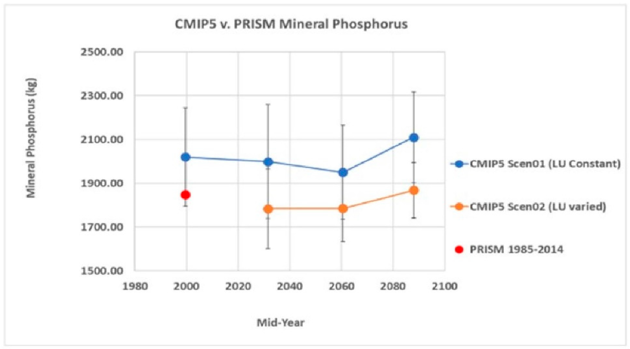
However, a reverse (decrease) trend was observed in mineral phosphorus from Scenario 1 to Scenario 2. The mean, median, minimum, and maximum values for mineral phosphorus in Scenario 1 are 2000, 1984, 1512, and 2455 kg, in Scenario 2 are 1784, 1799, 1383, and 2184 kg.

The same trend for Scenarios 1 and 2 described above was repeated in the mid-century and late-century climate windows.

3.5. Scenario 1 and Scenario 2 Inter-Annual Variability Results (1985–2100)

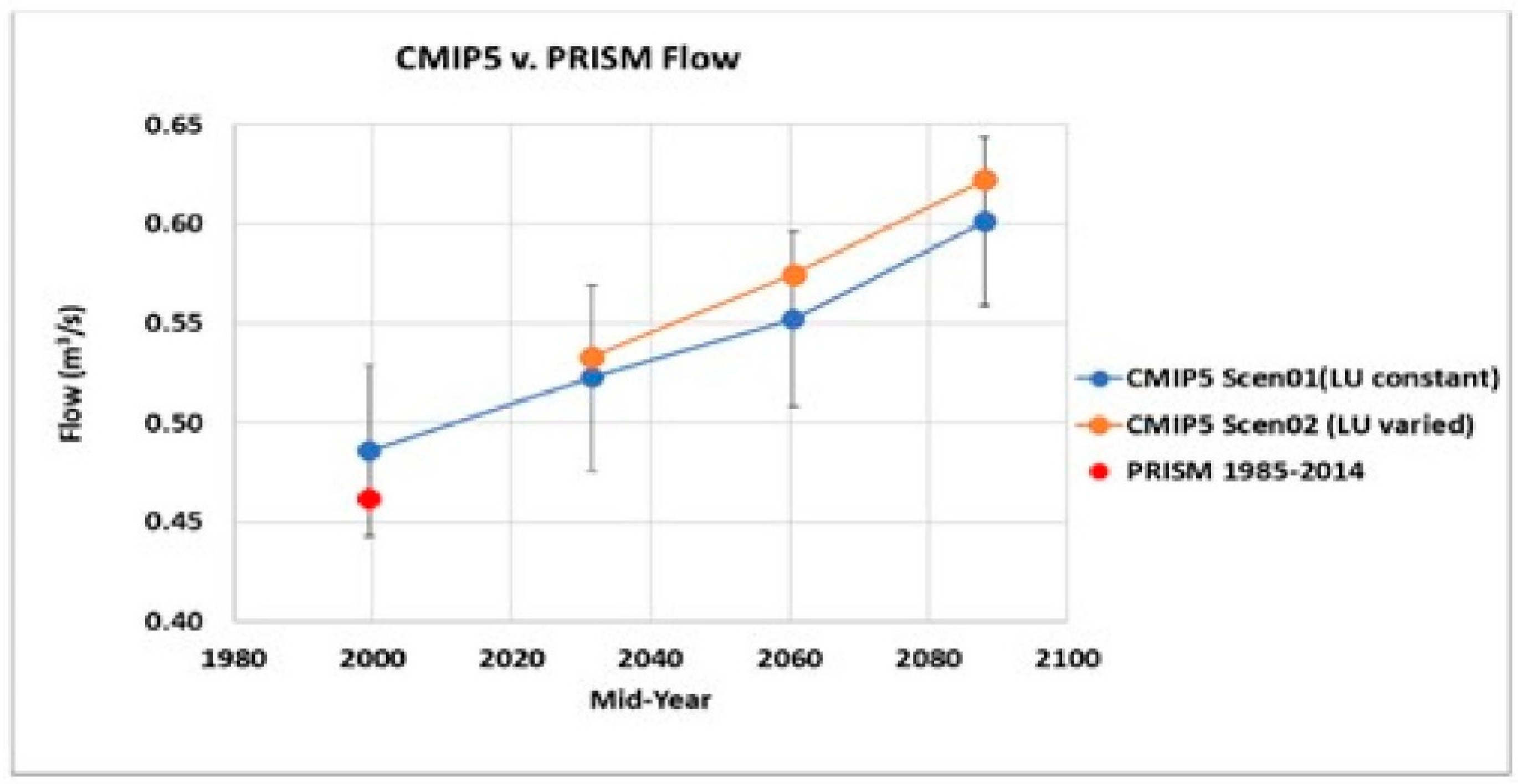
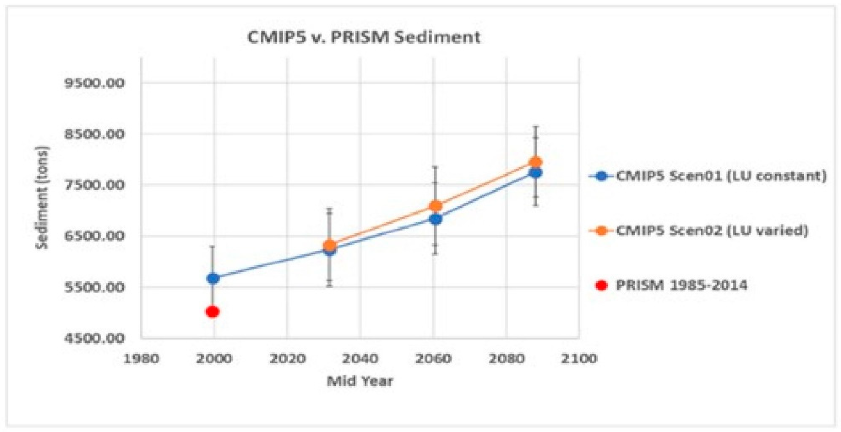
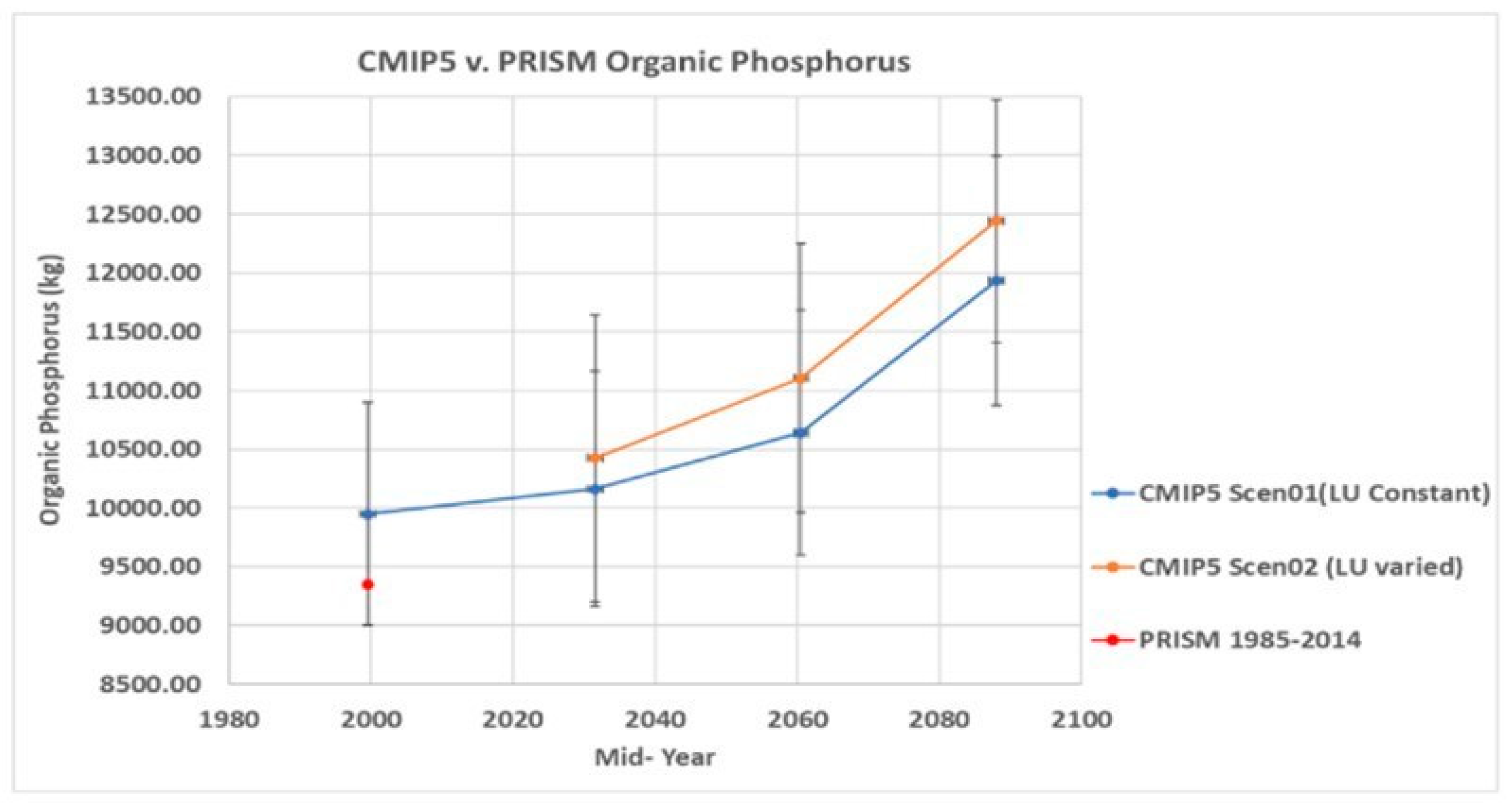
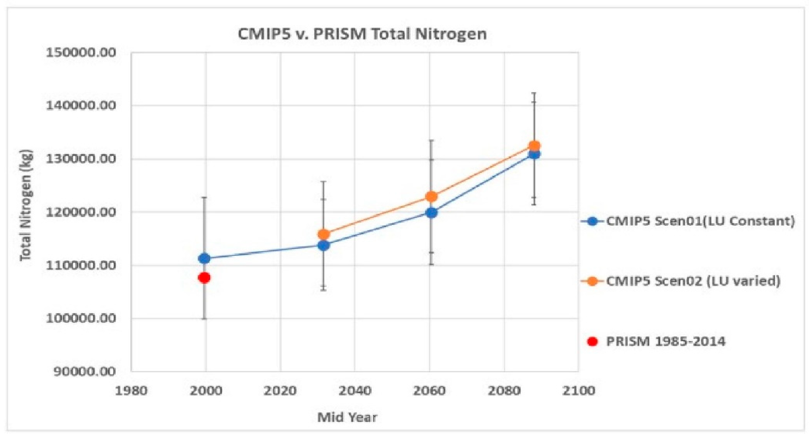
The results of the inter-annual variability analysis for Scenario 1 and Scenario 2 for all the 10 variables of interest are presented in Figure 4, Figure 5, Figure 6, Figure 7, Figure 8, Figure 9, Figure 10, Figure 11, Figure 12 and Figure 13. Flow and sediment show almost linear variability for the two scenarios across the century, but the effect of LULC is greater in flow than in sediment. Organic nitrogen and organic phosphorus show nonlinear increase for the two scenarios across the century with more increase towards the end of the century. The effect of LULC is more in organic phosphorus transport than in organic nitrogen. The effect of LULC created a decrease in mineral phosphorus (SRP) transport across the century as seen in Scenario 2. Chlorophyll a, CBOD, dissolved oxygen, total nitrogen, and total phosphorus also increase nonlinearly across the century with more increase towards the end of the century in chlorophyll a, CBOD, and total phosphorus. The error bars were constructed from the standard deviation of the simulated results and show the degree of variability in each result. The variability between two results is statistically insignificant when the vertical error bars overlap and statistically significant when the vertical error bars do not overlap. For all the variables in the historical climate window, the average of 20 CMIP5 results is consistent with PRISM results, but CMIP5 overestimated the variables compared to PRISM, within the error of SWAT simulation. For all climate windows, the trend of the variables in Scenarios 1 and 2 are the same, the trend of the variable is controlled by climate, which is common to both scenarios, while the effect of LULC change is seen as the difference between the plots in the two scenarios. In Scenario 2, the expected slight changes in land use (−3.6% in agriculture and +2.4% in urbanization) across the century generated an increase in the streamflow and other water quality variables except for mineral phosphorus. The flow and nutrients increase annually from current–future to late-century climate window.

Table 6. Percentage change in the simulated variables relative to the historical climate window across the century.

Dataset	Mid-Year	Flow (%)	Sediment (%)	Organic Nitrogen (%)	Organic Phosphorus (%)	Mineral Phosphorus (%)
20 CMIP5 GCMs 1985–2014	1999.50	-	-	-	-	-
20 CMIP5 GCMs Scenario 1_2018-45	2031.50	7.59	9.79	3.88	2.14	−1.02
20 CMIP5 GCMs Scenario 2_2018-45	2031.50	9.69	11.51	4.94	4.79	−11.68
20 CMIP5 GCMs Scenario 1_2046-75	2060.50	13.64	20.55	8.02	6.94	−3.47
20 CMIP5 GCMs Scenario 2_2046-75	2060.50	18.28	24.85	9.56	11.62	−11.63
20 CMIP5 GCMs Scenario 1_2076-00	2088.00	23.76	36.66	17.93	19.96	4.45
20 CMIP5 GCMs Scenario 2_2076-00	2088.00	28.06	40.13	20.09	25.07	−7.51
Dataset	Mid-Year	Chlorophyll a (%)	CBOD (%)	Dissolved Oxygen (%)	Total Nitrogen (%)	Total Phosphorus (%)
20 CMIP5 GCMs 1985–2014	1999.50	-	-	-	-	-
20 CMIP5 GCMs Scenario 1_2018-45	2031.50	6.40	10.99	6.98	2.25	1.60
20 CMIP5 GCMs Scenario 2_2018-45	2031.50	7.99	12.48	9.04	4.11	2.01
20 CMIP5 GCMs Scenario 1_2046-75	2060.50	9.41	20.41	9.84	7.74	5.18
20 CMIP5 GCMs Scenario 2_2046-75	2060.50	12.01	22.71	13.76	10.42	7.70
20 CMIP5 GCMs Scenario 1_2076-00	2088.00	22.10	39.58	14.06	17.67	17.34
20 CMIP5 GCMs Scenario 2_2076-00	2088.00	22.97	43.34	18.96	19.08	19.57

shows the percentage change in the simulated variables relative to the historical climate window for both Scenarios 1 and 2 across the century. In the current–future climate window, the highest increase was observed in the Scenario 2 simulation for CBOD with 12.48% followed by sediment transport with 11.51%. In the mid-century climate window, Scenario 2 simulation for sediment transport yielded the highest increase at 24.85% followed by CBOD at 22.71%. In the late-century climate window, CBOD was highest at 43.34% followed by sediment transport at 40.13%. Total phosphorus gave the lowest increase across the century, while mineral phosphorus decreased across the century.

3.6. Relationship between Variables

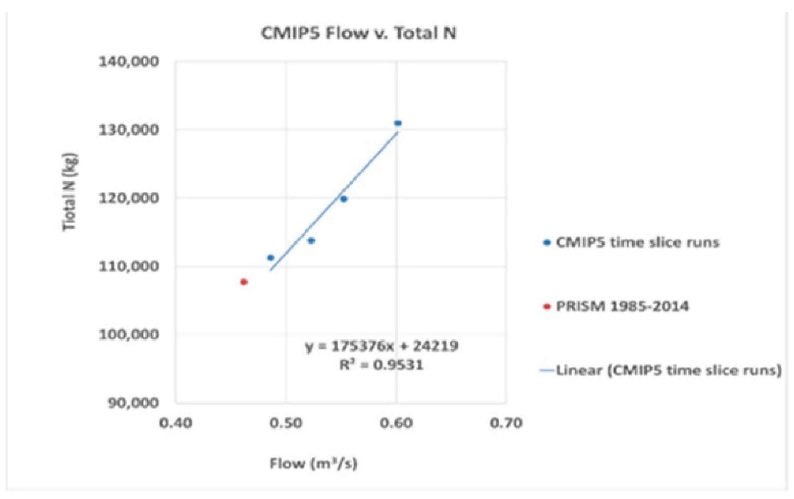
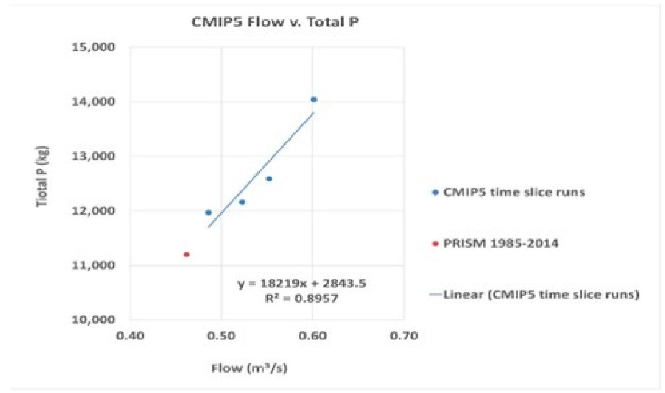
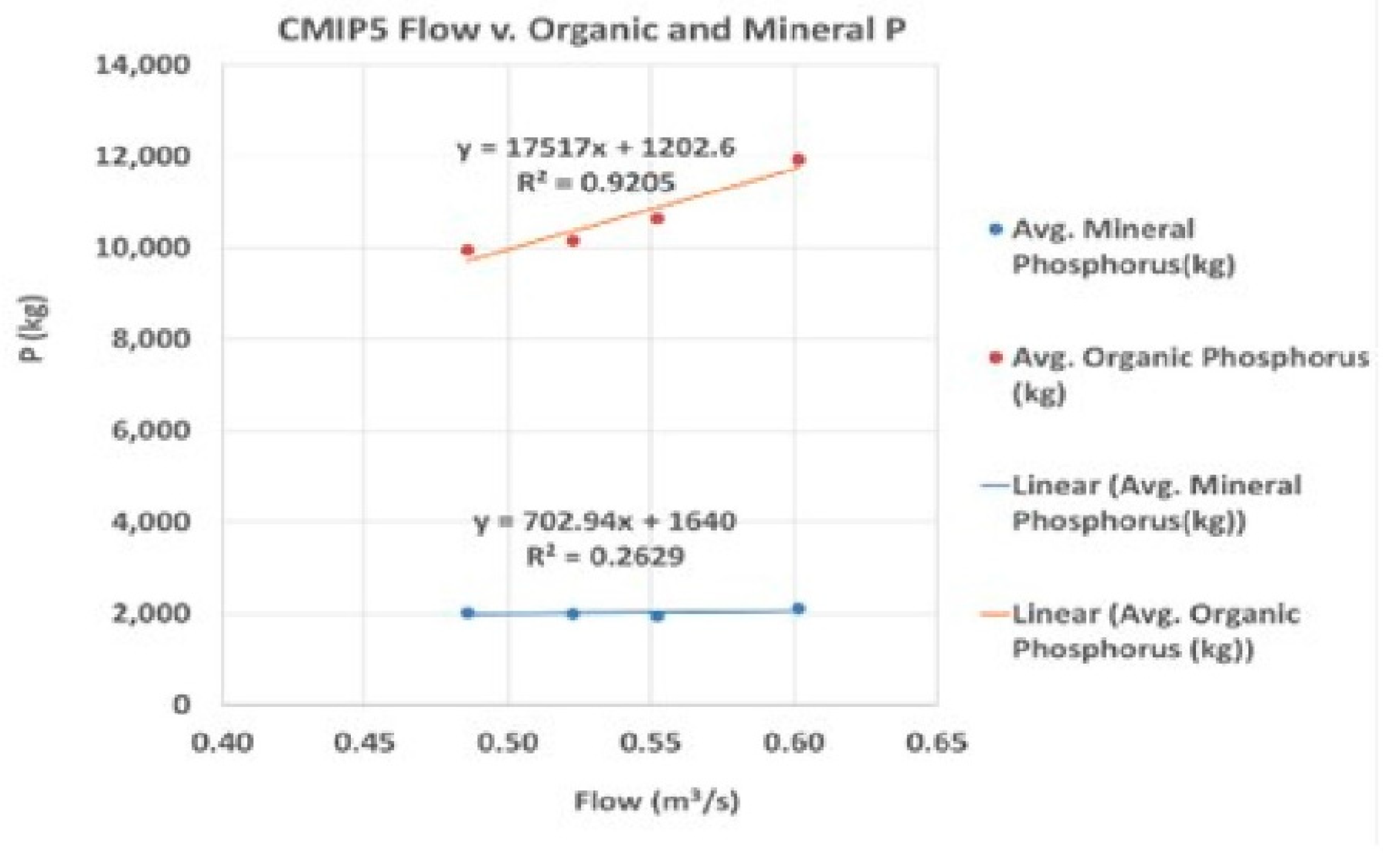
Cross plots were made between flow and water quality variables (Figure 14, Figure 15, Figure 16 and Figure 17). Flow is highly correlated with sediment across all the climate windows with R² value of 0.99. This shows that flow controls the sediment and that explains the similar trend between flow and sediment across the climate windows. Flow also correlated well with total nitrogen, total phosphorus, and organic phosphorus with strong R² values of 0.95, 0.90, and 0.92, respectively, but shows no correlation with mineral phosphorus. Apparently, the projected increase in flow is expected to lead to an increase in water quality variables that are positively correlated with flow across the climate windows.

4. Discussion

For the historical climate window, the average of the 20 CMIP5 GCMs’ results is a better predictor of the PRISM results than the individual results of the 20 GCMs model, and hence, the 20 GCMs can be used to run simulations for the future climate windows.

For Scenarios 1 and 2’s inter-model variability result, the effect of the projected climate change, which is (+13%) in precipitation and temperature (+47%), is seen in Scenario 1. The slight increase in streamflow and water quality variables in Scenario 2 relative to Scenario 1 is attributed to the effect of (+0.58%) in urbanization seen in Scenario 2, which increases surface runoff. A decrease in agricultural land makes less land available for infiltration, which increases flow. The synergistic effect of a 0.8% decrease in agricultural land and 0.58% increase in urbanization in Scenario 2 would, therefore, increase flow and sediment transport.

The effect of the slight increase in urbanization and slight decrease in agriculture in Scenario 2 compared to 1 appears to be more in nutrient transport than in flow and sediment transport.

The reduction in mineral phosphorus (SRP) in Scenario 2 relative to Scenario 1 is attributed to the dissolution and the addition of the mineral phosphorus to the total phosphorus. This was evident by the associated reduction in crop yield across the climate windows. Hence, more mineral phosphorus is being dissolved, thereby increasing the concentration of total phosphorus in the estuary. The increase in other nutrients would drive more eutrophication leading to anoxic condition within the estuary.

For Scenarios 1 and 2’s inter-annual variability result, the increase in flow drives sediment and nutrients transport. The projected high increase in CBOD and sediment transport will deteriorate the water quality, high total suspended sediment would affect water clarity, and high CBOD content would affect the dissolved oxygen content. As for mineral phosphorus, the effect of the projected change in agricultural land use in Scenario 2 (−3.6% in agriculture) created a decrease in the quantity of the mineral phosphorus transported relative to Scenario 1. The reduction in mineral phosphorus (SRP) is attributed to the dissolution and addition of mineral phosphorus in the system to the total phosphorus content. Mineral phosphorus is the only water quality variable that decreased from Scenario 1 to Scenario 2. The effect of the projected changes in LULC results in a small impact relative to the effect of climate change.

Similar results have been obtained by other researchers. Michalak et al. [26] carried out hydrological modeling of the Maumee River basin using SWAT and found an estimated increase in sediment and nutrient transport associated with the projected climate change. Du et al. [27] used SWAT modeling to evaluate the impact of LULC and climate change on runoff in the Dagu River basin in China and found out that the impact of LULC was lower than that of climate.

In this analysis, the most affected variables are streamflow, sediment transport, and CBOD. High stream flow would increase the vulnerability of the stream to flooding and would also increase sediment transport. High sediment transport would increase water turbidity and disrupt some aquatic habitats. High CBOD will lower the dissolved oxygen level in the water leading to the loss of aquatic lives. The results obtained from this work as shown by the cross plot are similar to those obtained by Stumpf et al. [28,29], who created models that forecast cyanobacteria bloom in Lake Erie using the Maumee River discharge and total phosphorus load.

The stochastic uncertainty of the model results for the OWC watershed is explained based on the previous analysis made by Evenson et al. [30]; they used five newly constructed watershed-scale models consisting of four SWAT models and one spatially referenced regression on watershed attributes (SPARROW) model, with different structure, input sources, and parameterization to assess the critical source areas (CSAs) uncertainty in the Maumee River watershed. Similar to the OWC watershed, the Maumee River watershed is a tributary of Lake Erie, primarily dominated by agricultural land use (~70%), which releases high phosphorus loads to the Lake Erie [31,32]. They observed a weak-to-moderate correlation in the sub watersheds of the five models, an agreement in the CSAs subset location, and a weak agreement in the CSAs location among five models. They attributed CSA uncertainty to the structural differences in the models and noted that the presence of uncertainty does not mean that the results of the simulations cannot be used for its intended purpose. All possible sources of model uncertainty should be evaluated using several models produced by different research organizations [30].

In this regard, the results of this analysis may be biased by model and climate uncertainties, which could be eliminated by comparing with similar results from other sources before use in decision making.

5. Conclusions

For the historical climate window results, the average of the 20 CMIP5 GCMs’ results for all the 10 variables of interest are more consistent with the PRISM results than each of the 20 individual GCMs’ results, and thus, the average is a better predictor of the PRISM results within acceptable error of SWAT simulation. The variability is smaller in the average of the 20 GCMs’ results being the average of 20 different results compared to the PRISM result, which is one.

For the current-to-future climate window, the results of Scenario 1 represent the effect of the projected climate change only. In Scenario 2, the slight increase in urbanization would increase surface runoff, and the slight decrease in agriculture would make less land available for infiltration, thereby increasing flow. Although these changes are not statistically different given the uncertainty in the model estimates, the synergistic effect of increasing urbanization and decreasing agricultural land is observed as an increase in flow, sediment transport, organic nitrogen transport, organic phosphorus transport, total nitrogen, and total phosphorus. Decrease or loss of mineral phosphorus observed in Scenario 2 relative to Scenario 1 is attributed to the dissolution of mineral phosphorus.

The progressive increase observed in flow and eight water quality variables across the century shows that there would be greater eutrophication and anoxic condition, which would further deteriorate the water quality in OWC estuary as time goes on. The flow controls the sediment and nutrient transport. Higher flow and nutrient transport are predicted for the future climate windows. Comparison between Scenarios 1 and 2 shows that the projected LULC change in the 21st century has a smaller impact on the water quality of Old woman creek compared to climate change.

Finally, the synergistic effect of the projected climate and LULC change observed in Scenario 2 increases across the climate windows. Not all the increase observed in nutrients would settle in the OWC estuary; a proportion would be transported into Lake Erie. The increase would drive proportional increase in eutrophication in both the OWC estuary and Lake Erie, thereby further deteriorating the water quality in the OWC estuary and Lake Erie.

The results of this work would assist the Huron and Erie counties in making policies relating to the land use management within the OWC watershed. It would assist the Ohio Department of Natural Resources (ODNR) and the management of OWC (NERR) in policies that would foster better management of the OWC estuary. It would assist the Ohio coastal management agencies in water quality studies in Lake Erie. The result would also serve as a reference for water quality studies in watersheds with dominantly agricultural land use in the United States and across the world.

References

- Scanlon, B.R.; Reedy, R.C.; Stonestrom, D.A.; Prudic, D.E.; Dennehy, K.F. Impact of land use and land cover change on groundwater recharge and quality in the southwestern US. Glob. Chang. Biol. 2005, 11, 1577–1593. [Google Scholar] [CrossRef]
- Schilling, K.E.; Jha, M.K.; Zhang, Y.-K.; Gassman, P.W.; Wolter, C.F. Impact of land use and land cover change on the water balance of a large agricultural watershed: Historical effects and future directions. Water Resour. Res. 2008, 44. [Google Scholar] [CrossRef]
- Fu, B.J.; Chen, L.D.; Ma, K.M.; Zhou, H.F.; Wang, J. The relationships between land use and soil condi-tions in the hilly area of the loess plateau in northern Shaanxi, China. Catena 2000, 39, 69–78. [Google Scholar] [CrossRef]
- Getachew, H.; Melesse, A. The impact of land use change on the hydrology of the Angereb watershed, Ethiopia. Int. J. Water Sci. 2012, 1, 1–7. [Google Scholar]
- Gwate, O.; Woyessa, Y.; Wiberg, D. Dynamics of land cover and impact on streamflow in the Modder River Basin of South Africa: Case study of a Quaternary catchment. Int. J. Environ. Prot. Pol. 2015, 3, 31–38. [Google Scholar]
- Gebremicael, T.; Mohamed, Y.; Betrie, G.; van der Zaag, P.; Teferi, E. Trend analysis of runoff and sediment fluxes in the Upper Blue Nile basin: A combined analysis of statistical tests, physically-based models and landuse maps. J. Hydrol. 2013, 482, 57–68. [Google Scholar] [CrossRef]
- Radeloff, V.C.; Hammer, R.B.; Stewart, S.I. Rural and Suburban Sprawl in the U.S. Midwest from 1940 to 2000 and Its Relation to Forest Fragmentation. Conserv. Biol. 2005, 19, 793–805. [Google Scholar] [CrossRef]
- Mishra, V.; Cherkauer, K.A.; Niyogi, D.; Lei, M.; Pijanowski, B.C.; Ray, D.K.; Bowling, L.C.; Yang, G. A regional scale assessment of land use/land cover and climatic changes on water and energy cycle in the upper Midwest United States. Int. J. Clim. 2010, 30, 2025–2044. [Google Scholar] [CrossRef]
- Niyogi, D.; Holt, T.; Zhong, S.; Pyle, P.C.; Basara, J. Urban and land surface effects on the 30 July 2003 mesoscale convective system event observed in the southern Great Plains. J. Geophys. Res. Space Phys. 2006, 111. [Google Scholar] [CrossRef]
- Alberti, L.; Cantone, M.; Colombo, L.; Oberto, G.; La Licata, I. Assessment of aquifers groundwater storage for the mitigation of climate change effects. Rend. Online Della Soc. Geol. Ital. 2016, 39, 89–92. [Google Scholar] [CrossRef]
- Oberto, G.; Alberti, L.; Sessa, R.S.; Colombo, L. Coupled irrigation-system/groundwater flow modelling for groundwater resource assessment in agricultural areas: A case study in northern Italy. Rend. Online Della Soc. Geol. Ital. 2018, 46, 94–100. [Google Scholar] [CrossRef]
- Bhattarai, G.; Hite, D.; Hatch, U. Estimating the Impact on Water Quality under Alternate Land Use Scenarios: A Watershed Level BASINS-SWAT Modeling in West Georgia, United States. In Efficient Decision Support Systems—Practice and Challenges in Multidisciplinary Domains; Jao, C.S., Ed.; InTech: Rijeka, Croatia, 2011. [Google Scholar]
- Fall, S.; Niyogi, D.; Gluhovsky, A.; Pielke, R.A.; Kalnay, E.; Rochon, G. Impacts of land use land cover on temperature trends over the continental United States: Assessment using the North American Regional Reanalysis. Int. J. Clim. 2009, 30, 1980–1993. [Google Scholar] [CrossRef]
- Bewket, W. Land Cover Dynamics Since the 1950s in Chemoga Watershed, Blue Nile Basin, Ethiopia. Mt. Res. Dev. 2002, 22, 263–269. [Google Scholar] [CrossRef]
- Lambin, E.; Geist, H.; Lepers, E. Dynamics of land use and land cover change in tropical regions. Annu. Rev. Environ. Resour. 2003, 28, 206–232. [Google Scholar] [CrossRef]
- Herdendorf, C.E.; Klarer, D.M.; Herdendorf, R.C. The Ecology of Old Woman Creek, Ohio: An Es-Tuarine and Watershed Profile, 2nd ed.; Ohio Department of Natural Resources, Division of Wildlife: Columbus, OH, USA, 2006.
- Olaoye, I.; Confesor, R.; Ortiz, J. Impact of Seasonal Variation in Climate on Water Quality of Old Woman Creek Watershed Ohio Using SWAT. Climate 2021, 9, 50. [Google Scholar] [CrossRef]
- Yang, W.; Andréasson, J.; Graham, L.P.; Olsson, J.; Rosberg, J.; Wetterhall, F. Distribution-based scaling to improve usability of regional climate model projections for hydrological climate change impacts studies. Hydrol. Res. 2010, 41, 211–229. [Google Scholar] [CrossRef]
- Neitsch, S.L.; Arnold, J.G.; Kiniry, J.R.; Srinivasan, R.; Williams, J.R. Soil and Water Assessment Tool User’s Manual Version 2000; TWRI Report TR-192; Texas Water Resources Institute: College Station, TX, USA, 2000; Volume 202.
- Arnold, J.G.; Srinivasan, R.; Muttiah, R.S.; Williams, J.R. Large area hy-drologic modeling and as-sessment–Part 1: Model development. J. Am. Water Resour. Assoc. 1998, 34, 73–89. [Google Scholar] [CrossRef]
- Gull, S.; Ma, A.; Dar, A.M. Prediction of Stream Flow and Sediment Yield of Lolab Watershed Using SWAT Model. J. Waste Water Treat. Anal. 2017, 8, 265. [Google Scholar] [CrossRef]
- Di Luzio, M.; Srinivasan, R.; Arnold, J.G.; Neitsch, S.L. ArcView Interface for SWAT2000: User’s Guide; TWRI Report TR-193; Texas Water Resources Institute: Forney, TX, USA, 2002.
- Confesor, R.B., Jr.; Whittaker, G.W. Automatic Calibration of Hydrologic Models with Multi-Objective Evolutionary Algorithm and Pareto Optimization. JAWRA J. Am. Water Resour. Assoc. 2007, 43, 981–989. [Google Scholar] [CrossRef]
- R-Development-Core-Team. R: A Language and Environment for Statistical Computing; R Foundation for Statistical Computing: Vienna, Austria, 2011; Available online: http://www.r-project.org (accessed on 31 January 2019).
- Nash, J.E.; Suttcliffe, J.E. River Flow Forecasting Through Conceptual Models—Part I: A Discussion of Principles. J. Hydrol. 1970, 10, 282–290. [Google Scholar] [CrossRef]
- Michalak, A.M.; Anderson, E.J.; Beletsky, D.; Boland, S.; Bosch, N.S.; Bridgeman, T.B.; Chaffin, J.D.; Cho, K.; Confesor, R.; Daloglu, I.; et al. Record-setting algal bloom in Lake Erie caused by agricultural and meteorologi-cal trends consistent with expected future conditions. Proc. Natl. Acad. Sci. USA 2013, 110, 6448–6452. [Google Scholar] [CrossRef] [PubMed]
- Du, F.-H.; Tao, L.; Chen, X.-M.; Yao, H.-X. Runoff Simulation Using SWAT Model in the Middle Reaches of the Dagu River Basin. In Sustainable Development of Water Resources and Hydraulic Engineering in China; Dong, W., Lian, Y., Zhang, Y., Eds.; Springer: Cham, Switzerland, 2019. [Google Scholar]
- Stumpf, R.P.; Wynne, T.T.; Baker, D.B.; Fahnenstiel, G.L. Interannual Variability of Cyanobacterial Blooms in Lake Erie. PLoS ONE 2012, 7, e42444. [Google Scholar] [CrossRef]
- Stumpf, R.P.; Johnson, L.T.; Wynne, T.T.; Baker, D.B. Forecasting annual cyanobacterial bloom bio-mass to inform management decisions in Lake Erie. J. Great Lakes Res. 2016, 42, 1174–1183. [Google Scholar] [CrossRef]
- Evenson, G.R.; Kalcic, M.; Wang, Y.-C.; Robertson, D.; Scavia, D.; Martin, J.; Aloysius, N.; Apostel, A.; Boles, C.; Brooker, M.; et al. Uncertainty in critical source area predictions from watershed-scale hydrologic models. J. Environ. Manag. 2021, 279, 111506. [Google Scholar] [CrossRef]
- Manning, N.F.; Wang, Y.-C.; Long, C.M.; Bertani, I.; Sayers, M.J.; Bosse, K.R.; Shuchman, R.A.; Scavia, D. Extending the forecast model: Predicting Western Lake Erie harmful algal blooms at multiple spatial scales. J. Great Lakes Res. 2019, 45, 587–595. [Google Scholar] [CrossRef]
- Baker, D.; Confesor, R.; Ewing, D.; Johnson, L.; Kramer, J.; Merryfield, B. Phosphorus loading to Lake Erie from the Maumee, Sandusky and Cuyahoga rivers: The importance of bioavailability. J. Great Lakes Res. 2014, 40, 502–517. [Google Scholar] [CrossRef]
Figure 1.
Location map of Old Woman Creek watershed.
Figure 2.
PRISM vs. Average of 20 CMIP5 GCMs precipitation.
Figure 3.
PRISM vs. Average of 20 CMIP5 GCMs temperature.
Figure 4.
PRISM vs. average of 20 CMIP5 GCMs flow (2018–2100).
Figure 5.
PRISM vs. average of 20 CMIP5 GCMs sediment (2018–2100).
Figure 6.
PRISM vs. average of 20 CMIP5 GCMs organic nitrogen (2018–2100).
Figure 7.
PRISM vs. average of 20 CMIP5 GCMs organic phosphorus (2018–2100).
Figure 8.
PRISM vs. average of 20 CMIP5 GCMs mineral phosphorus (2018–2100).
Figure 9.
PRISM vs. average of 20 CMIP5 GCMs chlorophyll a (2018–2100).
Figure 10.
PRISM vs. average of 20 CMIP5 GCMs CBOD (2018–2100).
Figure 11.
PRISM vs. average of 20 CMIP5 GCMs dissolved oxygen (2018–2100).
Figure 12.
PRISM vs. average of 20 CMIP5 GCMs total nitrogen (2018–2100).
Figure 13.
PRISM vs. average of 20 CMIP5 GCMs total phosphorus (2018–2100).
Figure 14.
Average of 20 CMIP5 GCMs flow vs. sediment (2018–2100).
Figure 15.
Average of 20 CMIP5 GCMs flow vs. total nitrogen (2018–2100).
Figure 16.
Average of 20 CMIP5 GCMs flow vs. total phosphorus (2018–2100).
Figure 17.
Average of 20 CMIP5 GCMs flow vs. organic and mineral phosphorus (2018–2100).