Abstract
Studies have shown that salt concentrations are increasing in waterbodies such as lakes, rivers, wetlands, and streams in areas where deicers are commonly applied for winter road maintenance, resulting in degraded water quality. As the salt concentration varies spatially and temporally based on environmental and hydrological characteristics, we monitored high resolution (15 min) salt concentrations for a relatively long period (winter and spring season) at different sites (i.e., stream, urban-stream, roadside drain, and parking-lot drain) using multiple electric conductivity-based sensors. The salt concentrations were significantly different from each other considering individual sensors and different sites in both winter and spring seasons, which support past research results that concentration varies spatially. Parking-lot (1136 ± 674 ppm) and Roadside (701 ± 263 ppm) drain measured significantly higher concentration than for Stream (260 ± 60 ppm) and Urban-stream (562 ± 266 ppm) in the winter season. Similar trends were observed for the spring season, however, the mean concentrations were lower in the spring. Furthermore, salt concentrations were significantly higher during the winter (242 ± 47 ppm to 1695 ± 629 ppm) than for the spring (140 ± 23 ppm to 863 ± 440 ppm) season considering different sites, which have been attributed to the winter snow maintenance practice using deicers in past studies. All sites exceed the United States Environmental Protection Agency (USEPA) threshold (salt concentration higher than 230 mg/L) for chronic exposure level for 59% to 94% and 10% to 83% of days in winter and spring seasons, respectively. The study has highlighted the usefulness and advantages of high resolution (spatially and temporally) salt concentration measurement using sensor technology. Furthermore, the salt concentration in waterbodies can vary spatially and temporally within a small spatial scale, which may be important information for managing water quality locally. The high resolution measurements (i.e., 15 min) were helpful to capture the highest potential salt concentrations in the waterbody. Therefore, the sensor technology can help to measure high resolution salt concentrations, which can be used to quantify impacts of high salt concentrations, e.g., application of deicer for winter road maintenance on aquatic systems based on the criteria developed by USEPA.
1. Introduction
Salts are widely used as a deicers for winter road maintenance in the US and around the world, which help to move vehicles during snow/ice events. Most of the salt applied for winter maintenance (over roads or parking lots) is later dissolved in the snow/rain melt runoff and infiltrates to contaminate surface and ground waters [1,2]. However, several other sources also contribute salt in waterbodies such as agricultural fertilizer, wastewater discharge, and industrial discharges, deicers, and natural salt sources, etc. [3,4]. The application of road salts has been increased with urbanization [5]. As the application of road deicers is increasing, there is evidence of increased chloride concentration in soil layers, surface water [1,6,7,8], groundwater [9,10]; and lakes [11], which ultimately affects water quality.
Generally, salt concentrations are monitored in waterbodies for a specific time by collecting samples and analyzing them in a lab, which is labor-intensive [12,13]. Nevertheless, salt concentration changes spatially and temporally depending on local climatic conditions (rain and snow event) and flows [14]. Recently, sensor technology has been used for continuous measurement of salt concentration, which is advantageous compared to the traditional method (sample collection), therefore useful to quantify the impacts of winter road maintenance using deicer on water quality [14,15,16,17,18,19]. The use of sensing technology, an alternative method that provides high-frequency data and real-time monitoring of water quality, is likely to increase in the future [20].
An increase in the concentration of salt in the soil causes an osmotic imbalance which will impede the plant water absorption, nutrient uptake, germination ultimately affecting plant growth [21,22]. The increase in salt concentration in surface water can cause adverse effects on aquatic organisms (terrestrial and aquatic biota) and overall ecosystems (i.e., aquatic and riparian) [23,24,25]. The studies have reported the richness and biodiversity in wetlands and waterways have been decreased due to an increase in sodium and chloride concentrations [3,26,27]. However, the macroinvertebrates are not affected by the level of sodium and chloride found in the wetlands [28]. These information show impacts of salt concentration on biotas living in aquatic system and environment, but the severity of impact may depend on the type of aquatic organisms [29,30]. The United States Environmental Protection Agency (USEPA) has set a threshold salt concentration criterion for ambient water, which should not be exceeded more than once in three years for healthy aquatic ecosystems. USEPA defined a chronic exposure level when moving four-day average concentration exceeds 230 mg/L and an acute level for concentration greater than 860 mg/L (one-hour average) [31].
The concentration of salt in the watershed also varies with time such as daily, monthly, and seasonally. Generally, the peak salt concentrations are observed during snow events in the winter months and decreased through the spring and summer months [9,14,29]. Large salt volume application during extremely high snowfall events results in considerably higher salt concentrations in streams and rivers than in winters with low snowfalls [9]. This seasonal variation and higher salt concentration in waterbodies during winter months are attributed to deicer application for winter road maintenance [5,12,30]. Furthermore, Researchers have observed higher salt levels during winter and continued through spring and summer months [30,32], which may be due to salt applied during the winter are stored in soil layers and then drain into streams/rivers during summer, when there are high rainfall and surface runoff [5,8,12,26]. Therefore, it is important to measure salt concentration continuously to capture the highest potential concentration in the environment.
The salt concentrations measured near roads in Illinois (USA) were extremely high and variable due to variability in deicer application rates, snowfall amounts, melting rates, etc. [30,33]. Salt concentrations were highest in waterbodies located in urbanized areas (e.g., the Chicago region) and lowest in streams with forested watersheds (e.g., Southern Illinois) and decreased exponentially with distance from highways/roadways [7,9,34]. The majority (about 96%) of deicer applications were accounted for roadways and parking lots, therefore, higher salt concentrations were observed in waterbodies near these locations [12,26,35]. Salt concentrations were significantly higher for low river discharges than for high discharges [33], therefore concentration depends on discharges (Corsi et al. 2010). The above examples showed that salt concentrations in waterbodies may vary spatially depending on discharges and watershed characteristics.
The study of spatial and temporal variations of salt concentrations is necessary to analyze their impacts on the environment and water quality management. High resolution measurements (e.g., hourly) are necessary to capture the highest potential salt concentration and to analyze an acute exposure level based on the criteria defined by the USEPA [31]. Most of the studies were focused on either national or regional or watershed (large) scale, so lacks information on spatial or temporal variation within the local (small) scale [14,29,33,34]. Because salt concentrations in waterbodies vary spatially and temporally and depend on many variables [29] (e.g., discharge, watershed characteristics, effluent from wastewater treatment plants and industries, etc.), the study results based on the large watershed scale may not be applicable for water quality management in a local (small) scale. To manage (reduce salt concentration) water quality locally by reactive approaches, for example using infiltration trenches, detention or retention ponds, wetland and shallow marshes, vegetated swales, and filter strips, etc. [36,37,38,39,40], the local salt concentration measurements should be considered instead of measurements based on the large spatial scale.
To fulfill the knowledge gap how salt concentrations vary spatially and temporally, we continuously measured high (15 min) resolution salt concentrations from November, 2018 to June, 2019 at multiple locations using a sensor-based approach. One of the major difference in our study from past studies are we analyzed salt concentration variations and differences spatially and temporally within and between multiple locations in a local (small) spatial scale (less than a 5 km radius). Furthermore, we analyzed the number of days that exceed the chronic exposure level for aquatic systems at different sites.
2. Methodology
2.1. Study Area
The study was focused on the city of Edwardsville and Glen Carbon, Madison County (IL, USA) which is located within the Illinois West Southwest climatological region [41] (Figure 1). The annual average rainfall in the watershed is 1050 mm and the mean annual snowfall is 300 mm. The total land area of Madison County is 1894 km2 and has 4486 km of paved surface roads [42]. The major road surfaces in Madison County are I-55, I-270 (interstate highways), IL-157 and IL-162 (state routes), county and municipal roads. Generally, roadside drains exist parallel to these roadways. There are numerous streams, roadside drains, and urban-streams in the watershed, which are ephemeral or perennial. Cahokia Creek, one of the largest creeks in the watershed, drains into the Mississippi River.
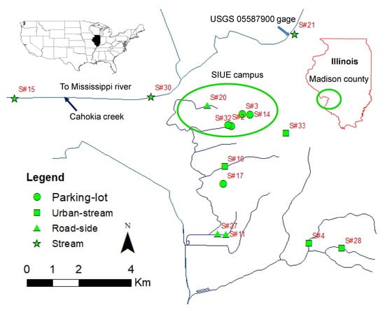
Figure 1.
Location of sensors at different waterbody sites (Stream, Urban-stream, Roadside drain, and Parking-lot drain) and USGS 05587900 gage. Sensor# 22 (Stream) and # 8 (Roadside) are not visible on the map due to scale adjustment.
2.2. Sensor Development and Field Deployment
We have developed sensors to measure salt concentrations by assembling a resistance-based carbon sensor that measures electrical conductivity (EC), data logger, battery, and microchip inside a polyvinyl chloride (PVC) housing [15,19]. The sensor measures EC, a proxy for salt concentration, water temperature, and atmospheric temperature [43,44,45]. Generally, the specific conductance/EC depends on the nature and type of ion present in water and temperature.
Sensors were calibrated and validated in a lab before their deployment in the field [15,19]. Furthermore, we also validated sensor measured field concentrations with a standard Hach conductivity meter manufactured by the Hach Company (https://www.hach.com/ accessed on 14 January 2021). The average errors between sensor and standard Hach meter salt concentrations were less than 5% but varied from 0 to 13% for the laboratory validation. Whereas average errors were between 9% to 12% and varied from 1% to 30% for field validations [15].
Salt concentrations in waterbodies vary spatially such as at near roads, urban areas, distance from highways/roadways and below parking lots, etc. [7,9,33,34,35]. Since, one of the main objectives of the study is to analyze spatial and temporal variability of salt concentrations within the site and between different sites, we deployed sensors at stream, urban-stream, roadside drain, and parking-lot drain locations. The locations for sensor deployment were selected based on the site available for sensor installation, safe from direct human reach, accessibility, and expected salt runoff during winter months. A total of 35 sensors were deployed in different locations around Madison County [19]. However, only 17 sensors were analyzed in this study because some of the deployed sensors were vandalized (three), malfunctioned (two), damaged due to excessive flow force (two), and dry locations (two) during most of the measurement period (Figure 1).
2.2.1. Stream
The stream site (Cahokia Creek) considered in this study is a perennial waterbody, where flow occurs all season. The study is focused on Cahokia Creek (about 35 m wide), which drains into the Mississippi River at the Lewis and Clark memorial park. The daily mean discharge is 4.15 m3/s based on the 50 years of records at the USGS 05587900 gage station. Most of the watershed (542 km2 at the gage station) area of the Cahokia Creek is a highly managed agricultural field including the city of Edwardsville, IL. A total of five sensors were deployed in Cahokia creek between the headwater (upstream of the city of Edwardsville) and the confluence with the Mississippi River, however, only four sensors were considered for the analysis. Sensor number (S#) 22 is located upstream of the city of Edwardsville, which has a mostly agricultural-dominated watershed, whereas the other three sensors (i.e., S# 21, 30, and 15) were located downstream from the city.
2.2.2. Urban-Stream
Urban-stream sensors were mainly deployed in the cities of Edwardsville and Glen Carbon. We considered a total of four such sensor measurements for the analysis. Although streams run through the urban areas, the majority of watershed areas are still occupied by agricultural fields and forests. State highways including other city roads, parking lots, and watersheds directly drain runoff in these streams during storm events. Therefore, we anticipated that these streams are exposed to a higher salt concentration since they run through urban areas. Most of these urban streams are perennial, but flows vary season to season based on rain/snowfall. For example, high flow occurs during the rain/snowfall event and is generally low during dry seasons.
2.2.3. Roadside Drain
The roadside drains are located parallel to the state highway (IL-157), interstate highways (I-270 and I-55), and other city roads. Most of these drains are ephemeral, and flow occurs mainly during rain and snow events. We analyzed four sensor measured salt concentrations for roadside drain, which were located within 10 m from the shoulder of roads. Salt mixed with runoff directly drains into these drains during winter road maintenance.
2.2.4. Parking-Lot Drain
These drains are located below the parking lot of the Southern Illinois University Edwardsville (SIUE), Edwardsville campus (Figure 1). These are ephemeral drains and therefore water flows only during the snow and storm events and mostly dry during non-rainfall events. We anticipated the highest salt concentrations in these drains because parking lots are heavily managed by applying salt during the winter season, specifically during snowfall events. A total of five sensors measured salt concentrations were analyzed for the parking-lot drains.
2.3. Data Analyses
The sensors were programmed in the Arduino platform (https://www.arduino.cc/ accessed on 14 January 2021). High-resolution (i.e., 15 min interval) digital data were downloaded in a “Text” format using the Arduino software and later converted into Microsoft Excel format [15]. These 15 min resolution data were converted into hourly and daily averages for further analyses. The temporal (seasonal) and spatial variations of measured salt concentrations. To analyze seasonal variation, measured data were classified into winter (December, January, and February) and spring (March, April, and May), whereas into parking-lot drain, roadside drain, urban-stream, and stream for spatial variations. We calculated the mean, range, standard deviation (SD), and coefficient of variation (CV) of measured salt concentrations.
Furthermore, null hypotheses were set to analyze if measured salt concentrations are significantly different spatially and temporally. A paired (two groups) permutation model was used to test if the null hypotheses are rejected (at α = 0.05) [46]. This approach analyzes if the dataset in the specific group is significantly different from another group.
Aquatic life exposed to a continuous level of 250 mg /L is considered harmful, whereas salt concentrations greater than 1000 mg/L can have toxic effects on aquatic plants and invertebrates [30]. Furthermore, the USEPA has set a threshold of 230 mg/L (four-day average) for chronic and 860 mg/L (one-hour average) acute levels to quantify impacts of salt concentration on the aquatic system [31]. This information showed that different criteria have been used to quantify the impacts of salt concentration on aquatic systems. To analyze the impact of salt concentrations on aquatic systems, we calculated an average number of days in each site, when concentrations (four-day moving average) were higher than the 230 mg/L thresholds set by the USEPA for ambient water for a chronic exposure level to aquatic biotas (hereafter chronic exposure) during winter and spring seasons and different sites [31]. Therefore, we calculated four-day moving average salt concentrations by filling missing values based on the linear interpolation [47]. Following null hypotheses (at α = 0.05) were set to compare salt concentration temporally and spatially.
2.3.1. Spatial Variation
- (i)
- The salt concentrations measured by individual sensors are not significantly different at various sites (i.e., parking-lot drain, roadside drain, urban-stream, and stream) during (a) winter, and (b) spring seasons
We used a paired permutation model to test the hypothesis. We compared concentration measured by an individual sensor to the concentrations for all other sensors in the spring and winter seasons. For example, if sensor number (S#) 100, 200, and 300 are used to measure concentrations at the specific site (e.g., parking-lot), concentrations were compared to each other for all three sensors for each season, which yield three-pair of comparisons (i.e., S# 100 Versus (Vs) S# 200, S# 100 Vs S# 300 and S# 200 Vs S# 300). If the null hypothesis is rejected, it states that concentrations based on the individual sensor are statistically significantly different from the concentrations based on another sensor at the site.
- (ii)
- The salt concentrations measured at various sites (i.e., parking-lot drain, roadside drain, urban-stream, and stream) are not significantly different during (a) winter, and (b) spring seasons
We considered all concentrations measured by multiple sensors in the site (e.g., parking-lot) as a group (hereafter “Overall-site”) for all sites (i.e., parking-lot drain, roadside drain, urban-stream, and stream) and separated into spring and winter seasons. To test the hypothesis, the concentrations at the specific site (e.g., parking-lot) were compared to concentrations at all other sites (e.g., roadside drain, urban-stream, and stream, etc.).
2.3.2. Temporal Variation
- (iii)
- The salt concentration measured between winter and spring seasons by individual sensors are not significantly different at various sites (i.e., parking-lot drain, roadside drain, urban-stream, and stream)
We compared concentrations between the winter and spring seasons for all individual sensors at all four sites to test the hypothesis. If the null hypothesis is rejected, it indicates that concentrations measured by different sensors between the winter and spring seasons are statistically significantly different.
- (iv)
- The salt concentrations measured between winter and spring seasons are not significantly different at various sites (i.e., parking-lot drain, roadside drain, urban-stream, and stream).
To test this hypothesis, we considered all concentrations measured by multiple sensors in a season (e.g., Winter) at the site (e.g., parking-lot) as a group (hereafter “Overall-season”. To test the hypothesis, the concentrations for the spring and winter at all sites were compared.
Furthermore, we also analyzed correlations between salt concentrations (measured at different sensor locations S# 15, 21, 22 and 30 in Stream) and measured discharges at the USGS 05587900 gage station in the Cahokia Creek (Figure 1). This also allowed to analyze, if concentrations change along the river from upstream to downstream. Previous studies have shown that salt concentrations depend on flow in rivers and locations of measurement (e.g., upstream or downstream) [29,33]. We further analyzed the difference in average, median, peak (highest), standard deviation, and variability (coefficient of variation) between hourly and daily averaged concentrations considering measurements at the Urban-stream.
3. Results
The daily average salt concentrations measured by individual sensors were spatially and temporally different in all sites (i.e., parking-lot drain, roadside drain, urban-stream, and stream) and seasons (i.e., winter and spring) (Figure 2). Generally, peak concentrations based on individual sensors were correlated with other sensors in each specific site. However, the time series between concentrations measured by individual sensors were different even those sensors were located in the same site (e.g., parking-lot). Concentrations were comparatively higher during the winter than the spring season in all sites. We presumed that the peak concentration was measured during the time of snowfall events when deicers were applied for winter road maintenance (Figure 2). In general, the highest salt concentrations were measured at the parking-lot drain and decreased at roadside drain, urban-stream and stream in chronological order. However, daily average concentrations were higher in urban-stream (specific for S# 10 and 28) than for roadside drain from 12 to 14 January 2019 (Figure 2).
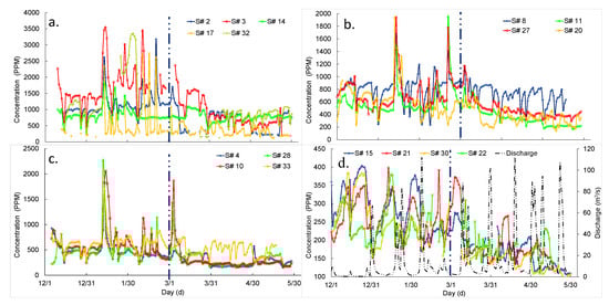
Figure 2.
Time series of daily average salt concentration from 1 December 2018 to 31 May 2019, at different sites: (a) parking-lot drain; (b) roadside drain; (c) urban-stream and (d) stream. Black dashed line (secondary axis) is discharge (m3/s) measured at USGS 05587900 gage station in Cahokia Creek. Blue dashed vertical line separates winter (December, January, and February) and spring (March, April, and May) seasons.
The daily average salt concentration decreased with higher discharges in a river (stream) during both winter and spring seasons (Figure 2d), although the trend lacks distinct correlations between discharge and salt concentrations. The coefficients of determination (R2) were between 0.07 to 0.18 for all sensors (i.e., S# 15, 21, 22, and 30). Salt concentration was noticeably higher during winter than for the spring for similar low discharges (e.g., less than 5 m3/s) (Figure 2d).
3.1. Spatial Variation
3.1.1. Parking-Lot Drain
The range of salt concertation variability was 30% to 115% based on the coefficient of variation (CV) at the parking-lot drain for the winter considering individual sensors (i.e., S# 2, 3, 14, 17, and 32). Based on the pair-wise permutation test, it rejected (p < 0.05) null hypothesis (i.e., measured concentrations are not significantly different) and accepted the alternative hypothesis (significant differences in concentration) for all comparisons, except for the pair S# 3 Vs S# 32 (Figure 3a). The mean concentrations for sensor# 3 and sensor# 32, were 1695 ± 629 ppm and 1436 ± 847 ppm, respectively, which were not significantly different (Figure 3a).
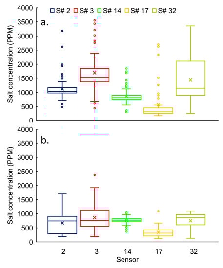
Figure 3.
Salt concentrations distribution at parking-lot drains for S# 2, 3, 14, 17, and 32 during (a) winter and (b) spring seasons. Box plot plotted by Microsoft Excel 2016, represents the lowest, highest, first quartile (25th percentile), median (50th percentile), third quartile (75th percentile) values of errors (%). The sign “X” and “○” represents the mean and outlier values, respectively. Lower and higher outliers are calculated by equations 25th percentile—1.5 × (75th percentile–25th percentile) and 75th percentile + 1.5 × (75th percentile–25th percentile), respectively.
The concentration variability in all sensors (S# 2, 3, 14, 17, and 32) was ranged from 18% to 52% in the spring (Figure 3b). The null hypothesis was rejected and the alternative hypothesis (significant differences in concentrations for all sensors) was accepted for most of the pair-wise comparisons (7 out of 10), except for S# 2 Vs S# 32, S# 3 Vs S# 32, and S# 14 Vs S# 32.
3.1.2. Roadside Drain
The concentration variability ranged from 27% to 43% at the roadside drain in winter for individual sensors (S# 8, 11, 27, and 20). We rejected (p < 0.05) null hypothesis (i.e., concentrations of individual sensors are not significantly different) and accepted the alternative hypothesis for the majority (four out of six) of pairs, except for S# 11 Vs S# 20 and S# 20 Vs S# 27 (Figure 4a). The mean concentrations for S# 11, 20, and 27, were 616 ± 263 ppm, and 743 ± 259 ppm, respectively, which were not significantly different (Figure 4a).
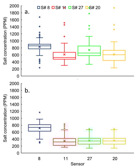
Figure 4.
Salt concentrations distribution at roadside drains for S# 8, 11, 27, and 20 during (a) winter and (b) spring seasons.
The concentration variability was ranged from 22% to 42% at roadside drain in winter (for S# 8, 11, 27, and 20) (Figure 4b). We rejected (p < 0.05) the null hypotheses (i.e., concentrations of individual sensors are not significantly different) for all sensors (pair-wise comparison), except for S# 11 Vs S# 20. Therefore, concentrations of individual sensors were significantly different from each other at the roadside drain. The mean concentrations for S# 11 and 20, were 348 ± 147 ppm and 359 ± 127 ppm, respectively, which were not significantly different (Figure 4b).
3.1.3. Urban-Stream
The concentration variability ranged from 31% to 58% at the urban-stream for all sensors (i.e., S# 4, 28, 10, and 33) in the winter (Figure 5a). Based on the permutation test, it rejected (p < 0.05) the null hypothesis for the majority (four out of six) of pair-wise comparisons, except for S# 10 Vs S# 33 and S# 4 Vs S# 28. Therefore, the tests indicated that concentrations of individual sensors were significantly different from each other. The means for S# 4 and 28 were 487 ± 203 ppm and 499 ± 289 ppm, respectively, which were not significantly different. Similarly, concentrations measured in S# 10 (616 ± 317 ppm) and 33 (645 ± 201 ppm) were not significantly different (Figure 5a).
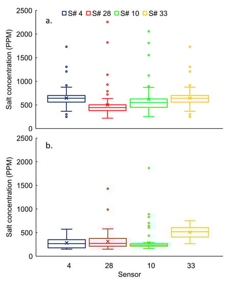
Figure 5.
Salt concentrations distribution at urban-stream for S# 4, 28, 10, and 33 during (a) winter and (b) spring seasons.
The concentration variability ranged from 24% to 75% at the urban-stream for all sensors (i.e., S# 4, 28, 10, and 33) in the winter. The permutation test rejected (p < 0.05) the null hypothesis for half of the pair-wise comparisons (three out of six). Therefore, concentrations of individual sensors were significantly different from each other in the half of pair-wise comparisons (S# 10 Vs S# 33, S# 28 Vs S# 33, and S# 3 Vs S# 33) and not in the rest of the pairs (S# 10 Vs S# 28, S# 4 Vs S# 10 and S# 4 Vs S# 28) at the urban-stream.
3.1.4. Stream
The mean concentrations varied from 242 ± 47 ppm to 281 ± 65 ppm. The concentration variability ranged from 20% to 25% (the smallest difference between upper and lower ranges) for all sensors (i.e., S# 15, 21, 22, and 30) at the stream in winter (Figure 6a). The null hypothesis was rejected (p < 0.05) for half (three out of six) of total pair-wise comparisons, except for S# 21 Vs S# 22, S# 21 Vs S# 30, and S# 21 Vs S# 30. The results indicated that the concentrations of individual sensors were not significantly different from each other for S# 21, 22, and 30 (Figure 6a).
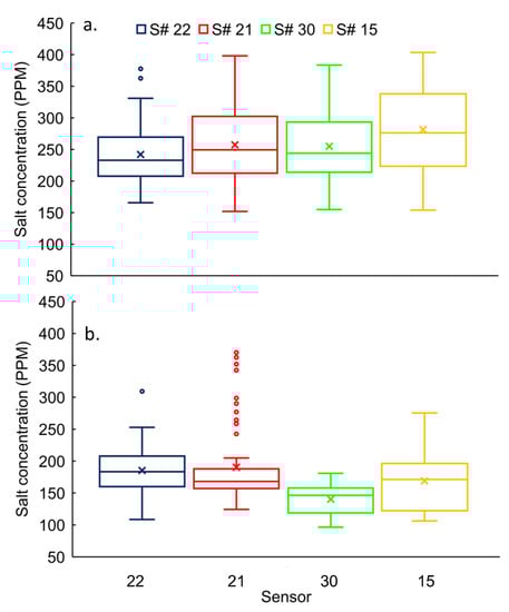
Figure 6.
Salt concentrations distribution at stream for S# 22, 21, 30 and 15 (from upstream to downstream) during (a) winter and (b) spring seasons.
For the spring, concentration variability ranged from 20% to 27% for all sensors at the stream (Figure 6b). Based on the permutation test, the null hypothesis was rejected (p < 0.05) for the majority of pair-wise comparisons, except for S# 21 Vs S# 22 (Figure 6b). The mean ± standard deviations for S# 21 and 22 were, 190 ± 60 ppm and 185 ± 37 ppm, respectively.
The daily mean salt concentrations were lowest at the farthest upstream sensor (S# 22) in the stream, where flow mostly drains from agricultural-dominated watershed than for other sensors (S# 15, 21, and 30) in the winter (Figure 6a). In general, concentrations increased along the river moving from upstream (S# 22) to downstream (S# 21, S# 30, and S# 15). The concentrations were highest at the farthest downstream among all sensors. However, salt concentrations did not follow the same trend during the spring season as in the winter (Figure 6). Daily mean concentrations were higher at the upstream (S# 22 and S# 21) than for the downstream (S# 30 and S# 15) in the spring (Figure 6b).
3.1.5. Overall-Site
The lowest mean concentrations were measured at stream (260 ± 60 ppm) and chronologically increased at urban-stream (562 ± 266 ppm), roadside (701 ± 263 ppm), and parking-lot (1136 ± 674 ppm) in winter for overall-site (Figure 7a). The concentration variability ranged from 23% to 59% for overall-site in the winter. Based on the permutation test, the null hypothesis was rejected (p < 0.05) for all pair-wise comparisons. Therefore, we could confidently state that concentrations were significantly different from one site to other sites for overall-site (Figure 7a).
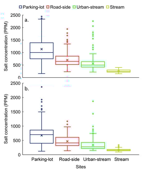
Figure 7.
Salt concentrations distribution for overall-site (parking-lot drain, roadside drain, urban-stream, and stream) during (a) winter and (b) spring seasons. The vertical axis is adjusted to 2500 ppm, therefore outliers (10) ranging from 2500 to 4000 are not visible in the figure.
As in the spring, the lowest concentrations were measured at stream in the winter and chronologically increased in urban-stream, roadside drain, and parking-lot in spring (Figure 7b). The concentration variability ranged from 29% to 51%. Based on direct comparison site by site, concentration variability increased in spring compared to winter at stream, urban-stream, and roadside, except for parking-lot, where it decreased. Similar in the winter, the null hypothesis was rejected (p < 0.05) for all pair-wise comparisons, which indicated that concentrations were significantly different from one site to another sites (Figure 7b).
3.2. Temporal Variation
3.2.1. Parking-Lot Drain
The mean ± standard deviation concentrations for all sensors (S# 2, 3, 14, 17, and 32) varied from 564 ± 646 ppm to 1695 ± 629 ppm at the parking-lot drain in the winter (Figure 3a). Whereas, the mean concentrations for all sensors varied from 342 ± 163 ppm to 863 ± 440 ppm in the spring (Figure 3b). The permutation test rejected (p < 0.05) the null hypothesis for all pair-wise (winter vs. spring) comparisons (individual sensors) for winter and spring. Therefore, there are significant differences (higher in winter) in concentration for all sensors (Figure 3a,b).
3.2.2. Roadside Drain
The mean concentrations varied from 616 ± 263 ppm to 827 ± 227 ppm at the roadside drain in winter (S# 8, 11, 27, and 20) (Figure 4a), whereas it varied from 348 ± 147 ppm to 714 ± 155 ppm in winter (for S# 8, 11, 27, and 20) (Figure 4b). However, means in all sensors were likely skewed by outliers in both seasons (Figure 4). Based on the permutation test, the null hypothesis (i.e., concentrations of individual sensors are not significantly different) was rejected (p < 0.05) for all pair-wise comparisons between winter and spring. Therefore, the concentrations in winter were significantly higher than in spring for all individual sensors at the roadside drain.
3.2.3. Urban-Stream
The mean concentrations varied from 487 ± 203 ppm to 499 ± 289 ppm at the urban-stream for all sensors (i.e., S# 4, 28, 10, and 33) in winter (Figure 5a), whereas., varied from 282 ± 106 ppm to 507 ± 121 ppm in the spring. Nevertheless, these means may have skewed by outliers (Figure 5a,b). The permutation test rejected (p < 0.05) null hypothesis for all pair-wise (winter vs. spring) comparisons. Therefore, our results indicated that concentrations in winter were significantly higher than for spring based on individual sensors.
3.2.4. Stream
The mean concentrations varied from 242 ± 47 ppm to 281 ± 65 ppm for all sensors (i.e., S# 15, 21, 22, and 30) at stream in winter (Figure 6a). For spring, the mean concentrations varied from 140 ± 23 ppm to 190 ± 60 ppm (Figure 6b). The null hypothesis test yielded salt concentrations were significantly higher in winter than in spring for all pair-wise comparisons.
3.2.5. Overall-Season
The mean concentrations were 260 ± 60 ppm (stream), 562 ± 266 ppm (urban-stream), 701 ± 263 ppm (roadside), and 1136 ± 674 ppm (parking-lot) for overall-season in winter (Figure 7a). For spring, the concentrations varied from 168 ± 49 ppm (stream), 341 ± 183 ppm (urban-stream), 467 ± 205 ppm (roadside), and 676 ± 342 ppm (parking-lot). Based on the permutation test, the null hypothesis was rejected (p < 0.05) for all pair-wise (winter vs. spring) comparisons. Therefore, it is concluded that concentrations were significantly different from one site to another and concentrations was significantly higher in winter than that of the spring season (Figure 7).
3.3. Hourly and Daily Averaged Concentration
The peak (highest) salt concentrations were higher in hourly averaged (from 15 min interval) values than for the daily and differences varied from 2 to 21% for the urban-stream (Figure 8, Table 1). The peak concentrations in the hourly data were diminished (decreased) noticeably in the daily averaged time series for all sensors (Figure 8), whereas the lowest concentrations were increased in daily averaged values. Nevertheless, the difference in average and median values was less than 2% for all sensors (Table 1).
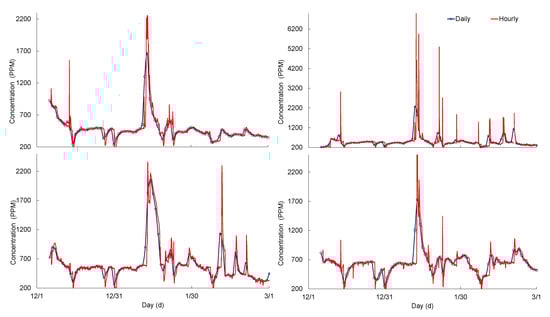
Figure 8.
Time series for hourly and daily averaged (calculated from 15 min interval data) salt concentrations for the winter season at the Urban-stream.

Table 1.
Change (relative to the hourly value) in salt concentration statistics (ppm) when values were averaged to hourly and daily from 15 min interval.
Standard deviations (SD) were higher for hourly averaged values than for the daily in all sensors, which varied from 8 to 25%. Therefore, the coefficient of variation (CV) was also altered as a result of a change in SD (Table 1). The hourly averaged concentration variabilities (based on CV) were noticeably higher than for the daily averaged values for all sensors (i.e., S# 4, 10, 28, and 33), which indicated that averaging the values may lead to different statistics of the data distributions.
3.4. Impacts on Aquatic System
We quantified a number of days for chronic exposure to analyze the impacts of salt concentrations on the aquatic system. The USEPA defined chronic exposure levels for aquatic biotas when four-day moving average salt concentrations are higher than 230 mg/L [31]. Chronic exposure levels were 84, 87, 87, and 53 days at the parking-lot drain, roadside drain, urban-stream, and stream, respectively, during the winter (total 90 days), whereas 76, 80, 64, and 9 days for the spring (total 92 days) (Figure 9). Chronic exposure levels were lowest in stream for both winter (53 days) and spring (9 days) compared to other sites. The chronic exposure levels were not noticeably different at parking-lot and roadside drains. Furthermore, chronic exposure levels were higher in winter than in the spring at all sites (Figure 9).
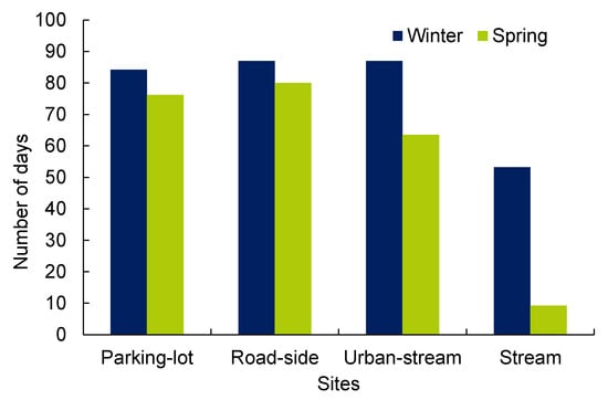
Figure 9.
Distribution of a chronic exposure level (number of days) at different sites (i.e., parking-lot drain, roadside drain, urban-stream, and stream) for winter and spring seasons when salt concentrations are higher than USEPA threshold of 230 mg/L in ambient water.
4. Discussion
We used salt concentration measurements (15 min temporal resolution) at different sites using multiple sensors to understand spatial and temporal variations. Sensor measurements were validated in both lab and field, where errors were within the permissible limit for field measurements [15,19]. Furthermore, Benjankar and Kafle [15] compared sensors (relatively close to each other) measured salt concentrations at roadside and stream locations, which were approximately 200 m and 50 m apart, respectively and they found salt concentrations were not statistically significantly different. These results further verify that sensor can be used confidently to measure salt concentrations in environments to analyze impacts of human activities (e.g., wastewater treatment plant and industrial discharge, use of agricultural fertilizer and deicers for winter road maintenance, etc.). The distribution of salt concentrations was temporally and spatially variable (168 ± 49 ppm to 1695 ± 629 ppm) among individual sensors and all sites as well as during the winter and spring seasons consistent with other studies (e.g., [14,48,49]). Salt concentrations varied nine times within a day during road-salt runoff periods (e.g., winter months) in a past study [50].
4.1. Spatial Variation
The measured salt concentrations were statistically significantly (p < 0.05) different from the sensor to sensor within the site (i.e., parking-lot drain, roadside drain, urban-stream, and stream) in the majority of pair-wise comparisons and both winter and spring seasons (Figure 2, Figure 3, Figure 4, Figure 5, Figure 6 and Figure 7). As with the individual sensors, concentrations were significantly different from one site to another (overall-site) (Figure 7). Salt concentration differences between two locations in a waterbody can be due to many factors such as distance between them, upstream or downstream locations, river discharge, groundwater flow, input from point sources (e.g., wastewater treatment plant, industrial discharge), use of agricultural fertilizer and deicers for winter road maintenance, watershed characteristics, and natural salt sources, etc. [3,29,33]. Other studies have found that the highest salt concentration in urbanized areas (e.g., the Chicago region) and the lowest in streams with forested watersheds [34,51]. However, a river with an agricultural watershed had a significantly higher chloride concentrations (86 mg/L) because of geological brine discharge than in the Sangamon River that has large cities as its watershed (34 mg/L) [51]. Therefore, it shows salt concentrations and distribution can be affected by many factors. We do not have information of any other specific sources in the study area that alters salt concentrations. However, based on past studies and observations, we could speculate that application of salt for winter road maintenance is the major driver for high salt concentrations in the waterbodies during winter season.
The highest salt concentration measurements for parking-lot drain among all other study sites in winter and spring seasons (Figure 7) were justifiable because the sensors are located directly below the parking-lot, where salts are used to manage the parking lot during winter. Although we do not have data to verify, we speculated that the application of deicers (salts) was noticeably higher in the SIUE parking-lots than the surrounding (e.g., roads). Furthermore, the sensor locations in parking-lot and urban-stream have a higher pavement to total watershed ratio compared to stream and roadside drains. Past studies have concluded that salt concentration increases with an increase in impervious surfaces [7,52,53]. Generally, large volumes of deicer are applied over pavement than for the natural watershed areas resulting in higher salt concentration in the nearby drain, which may explain why concentrations are higher for roadside and parking-lot drains. For example, a study found that the highest contribution of salt was from the parking lots (44%) followed by municipal roads (37%) and state roads (10%) [12,35].
Our study showed the lowest salt concentrations in stream compared to parking-lot, roadside drain, and urban-stream both in winter (260 ± 60 ppm) and spring (168 ± 49 ppm), which were consistent with other studies. The result (lowest concentration at stream site) could be due to a dilution effect in the stream (Cahokia Creek), where discharges were noticeably higher than other locations [1,52]. Nevertheless, concentrations were still higher than 230 mg/L (USEPA threshold for the chronic exposure level) in the stream which is similar to the observation at rivers in the Chicago region during the months of July–October (generally higher than 100 mg/L) [51]. Furthermore, salt concentration in the Illinois River decreased from upstream to downstream [33]. This can be an additional example of dilution effect on the spatially varying salt concentrations in a natural waterbody because generally, discharge increase as watershed area increase (upstream to downstream). However, there was no such trend along the Cahokia Creek (classified as stream) in the current study. The lowest salt concentrations were measured at the sensor located farthest upstream (S# 22) and increased along the river toward downstream during the winter season (Figure 6a). The majority of watershed areas for the farthest upstream sensor (S# 22) is agricultural land, whereas urbanized areas for downstream sensors (S# 21, 30 and 15). Therefore, we speculated that salt concentration increased at downstream locations due to salt-laden runoff contributions from the City of Edwardsville, where application of deicer occurred for winter road and parking lot maintenances. This statement may support by the evidence that there is no such trend in the spring season.
Based on our results and other studies, salt concentrations could be higher in ephemeral drains (e.g., parking-lot and roadside) than for the perennial streams (Cahokia Creek and urban-stream), which has generally higher discharges (larger watershed) and forested or agricultural watershed [34,51]. Studies have reported that salt concentrations were significantly higher during low discharge conditions, regardless of season (e.g., winter or spring) [33,52,54]. Our results were consistent with these studies where the highest salt concentrations were measured during low flows (e.g., less than 5 m3/s) than during high flows for both winter and spring seasons (Figure 2d). Nevertheless, relatively low coefficient of determination values (R2 = 0.07 to 0.18) indicated that discharge in the river alone do not explain the cause of variability in salt concentrations, specifically for the small watershed such as Cahokia Creek, where flows vary the order of magnitude within a day (Figure 2d).
We noticed that S# 3 was located at stagnant water at the parking-lot drain. We suspect that the sensor might have measured high concentrations continuously for a period until the occurrence of another rain event (Figure 2a and Figure 3). This result had shown that the deployment of sensors in probable stagnant water locations should be avoided for accurate measurements. Nevertheless, these results should not alter the outcome of this study.
4.2. Temporal Variation
The current study showed statistically significant higher salt concentration during winter for all four-study sites (i.e., parking-lot, urban-stream, roadside drain, and stream) considering individual sensors and different sites (Figure 2, Figure 3, Figure 4, Figure 5, Figure 6 and Figure 7). These results were consistent with other studies, where winter salt concentrations were significantly higher than other seasons, which were attributed to deicer applications for winter road maintenance [11,14,53]. Furthermore, the concentrations were lower in spring, which might indicate a change in the quantity of deicer application.
Our results are supported by several studies showing a positive correlation between chloride concentration and the application of deicers [6,7,51]. Salt concentrations were higher in the winter season and the concentration decreased as the application was stopped during the spring and summer months [51,53]. Nevertheless, salt concentrations in spring and summer months could be still high although the application of deicers is stopped because the salt applied during the winter could be stored in nearby soils and flushes into the waterbody from runoff generated by rainfall during spring and summer [12,29].
4.3. Impacts on Aquatic Systems
Based on the USEPA criteria, chronic exposure level (number of days) varied from 53 to 84 (59% to 94% of days) days for all sites in the winter season, whereas 9 to 80 days (10% to 87%) for the spring (Figure 8). The results showed the severity of the impacts of salt concentrations on the aquatic system. Although, mean salt concentration for parking-lot was higher for both winter (1136 ± 674 ppm) and spring (676 ± 342 ppm), chronic exposure level was higher for roadside drains (Figure 8). The result showed salt concentrations exceeded chronic exposure threshold levels of the USEPA in the majority of winter and spring period, which are similar in past studies (e.g., [14,29]). These studies had shown that excessive chloride concentration (as high as 7730 mg/L) in streams was a result of road salt runoff. Furthermore, chloride concentrations periodically exceeded chronic and acute chloride threshold levels of the USEPA criteria in most of the study sites in Toronto [14]. Higher chronic exposure levels during the winter than for the spring demonstrated a substantial impact of salt applications for winter road maintenance on water quality and aquatic systems [29]. Our results indicated that higher salt concentrations (e.g., 230 mg/L) can impact the aquatic system not only during winter but in spring as well [9,29,34].
High salt concentrations can have immediate or long-term effects on aquatic biota, which may eventually affect community structure, diversity, and productivity [27,30]. The lowest mean salt concentrations were measured at stream locations (260 ± 60 ppm) for the winter among all sites, which is still higher than 230 mg/L, a threshold for chronic exposure level for the aquatic system. Furthermore, the daily average concentrations were varied between 219 ppm (lowest) to 3548 ppm (Highest) in all sites, which showed the severity of impacts of salt concentrations on the aquatic system, but depends on species living in the system. Based on the long-term toxicity test on Ceriodaphnia dubia (C. dubia) in another study, initial toxic effects begin to observe between salt concentrations of 600 and 1100 mg/L, and mortality occurred at 2420 mg/L or higher [29]. Other effects of the salt concentrations on the aquatic organisms were no young production and weight loss.
Our study has shown that higher salt concentrations during the winter season consistent with past studies (e.g., [29,34]), which may impact biological integrity in urban waterbodies,. Past studies had analyzed impacts of high salt concentrations in aquatic system and organisms, but they were not based on continuous high resolution measurements, therefore, may not fully represent the severity of influence [26,34,55]. Therefore, our study supports the statement that due to the episodic nature, the full range of impacts of salt application on the aquatic system will be difficult to quantify, unless measurements are continuous and high resolutions [29]. The event-based, periodic or fixed-interval sampling approach may not fully characterize the extent of impacts of salt concentration in the environments.
4.4. Study Application
This study, along with past studies has demonstrated the usefulness and advantages of sensor technology to monitor high-resolution salt concentrations continuously [14,15,16,17,18]. Our study results were consistent with past studies where higher salt concentration are in the waterbodies located within urban areas and close to the road as well as higher salt concentrations in winter than in the spring [7,33,51,56]. These studies attributed higher salt concentrations during winter months to the application of deicer as winter road maintenance, but there could be multiple reasons for elevated salt concentration such as occurring naturally, wastewater treatment and industrial plant discharge, and agricultural practices. However, it is important to quantify all sources for elevated salt concentrations for water quality management.
Our study has shown that continuous high resolution (15 min) measurements are advantageous for capturing the highest potential salt concentrations in the waterbodies (Figure 8). Noticeably, averaging into longer duration (i.e., daily) may underestimate the real impacts of salt concentrations in the aquatic system. As expected, increasing the number of time-step intervals for calculating the daily averaged values has resulted in reduction in variabilities in concentration distributions and smoothened trends as observed in other studies (e.g., [57]). Therefore, our study showed the importance of high resolution (spatial and temporal scale) salt concentration measurements for quantifying chronic and acute exposure levels defined by the USEPA [31] based on the daily and hourly averaged values, respectively, as well as capturing the highest potential salt concentrations.
Although analyzing comprehensive impacts of salt concentration on aquatic biota is out of the scope of this study, it has shown that elevated salt concentrations in waterbodies specifically located in an urban setting are an important factor for the biological integrity of those waterbodies. We have shown the applicability and advantages of sensor technology to measure high resolution (spatially and temporally) salt concentrations. To manage/restore water quality by developing local structures such as detention or retention ponds, wetland, and shallow marshes, and vegetated swales, etc., the approaches presented in this study would be useful [36,37,38,39]. Therefore, we believe our study results would be helpful for agencies and managers who manage winter road maintenance and aquatic ecosystem projects.
5. Conclusions
Our results showed high variability of salt concentrations in spatial (different sites) and temporal (seasons) scales. The highest salt concentrations were found in drains directly below the parking lot in the winter (1695 ± 629 ppm), whereas the lowest (281 ± 65 ppm) concentrations were at perennial streams with relatively larger watersheds (Cahokia Creek) where flows are comparatively higher than other ephemeral drains (roadside and parking-lot drains). High salt concentrations were measured for low discharges, however, concentration variabilities might also depend on other drivers such as the source of salt input in the systems. There was a significant increase in mean salt concentration during the winter season (260 ppm to 1136 ppm) than in the spring (168 ppm to 676 ppm) in all sites. Such results have been attributed to the winter snow management practices using deicers in other studies. One of the important findings of this study is that the salt concentration in waterbodies can vary spatially and temporally in a small spatial scale (within a 5 km radius). The coefficients of variation (CV) were between 23% to 59% and 29% to 54% for winter and spring, respectively. The study has highlighted the importance of measuring high resolution (spatially and temporally) salt concentrations and the advantages of the use of sensor technology. Therefore, sensor technology can be a valuable tool to analyze the impacts of road salt applications on local waterbodies and aquatic systems.
Author Contributions
Conceptualization, R.B.; Data curation, R.K., S.S. and N.A.; Formal analysis, R.B., R.K. and S.S.; Funding acquisition, R.B.; Investigation, R.B. and R.K.; Methodology, R.B. and R.K.; Software, R.K.; Supervision, R.B.; Validation, R.B.; Writing—original draft, R.B. and R.K.; Writing—review & editing, R.B., R.K., S.S. and N.A. All authors have read and agreed to the published version of the manuscript.
Funding
This research received no external funding.
Institutional Review Board Statement
Not applicable.
Informed Consent Statement
Not applicable.
Data Availability Statement
The data presented in this study are available on request from the corresponding author.
Acknowledgments
Funding for this study is provided through the School of Engineering (New faculty Start-up) and the Graduate School’s “Research Equipment and Tools” funding programs. We would like to acknowledge the Center for Ecohydraulics Research (CER), University of Idaho, and Bob Basham for developing sensors as part of the collaborative research. Furthermore, we are also thankful to Brent Vaughn, Lab manager at the School of Engineering, SIUE, and students Victoria Wieseman and Utsav Manandhar for helping in this project. We appreciate the cooperation from Region Five District 8, Department of Transportation, Collinsville, IL for granting permission to deploy sensors near roads. We would like to acknowledge the comments from three anonymous reviewers and editors. The comments helped to improve the manuscript quality.
Conflicts of Interest
The authors declare no conflict of interest.
References
- Thunqvist, E.-L. Regional increase of mean chloride concentration in water due to the application of deicing salt. Sci. Total Environ. 2004, 325, 29–37. [Google Scholar] [CrossRef]
- Jamshidi, A.; Goodarzi, A.R.; Razmara, P. Long-Term impacts of road salt application on the groundwater contamination in urban environments. Environ. Sci. Pollut. Res. 2020, 27, 30162–30177. [Google Scholar] [CrossRef]
- Panno, S.; Hackley, K.C.; Hwang, H.; Greenberg, S.; Krapac, I.; Landsberger, S.; O’Kelly, D. Source Identification of Sodium and Chloride Contamination in Natural Waters: Preliminary Results. In Proceedings of the 12th Annual Illinois Groundwater Consortium Symposium, Makanda, IL, USA, 22 April 2003; Illinois Groundwater Consortium: Champaign, IL, USA, 2003. [Google Scholar]
- Müller, A.; Österlund, H.; Marsalek, J.; Viklander, M. The pollution conveyed by urban runoff: A review of sources. Sci. Total Environ. 2020, 709, 136125. [Google Scholar] [CrossRef]
- Corsi, S.; Cicco, L.A.; ALutz, M.; MHirsch, R. River chloride trends in snow-affected urban watersheds: Increasing concentrations outpace urban growth rate and are common among all seasons. Sci. Total Environ. 2015, 508, 488–497. [Google Scholar] [CrossRef]
- Godwin, K.; Hafner, S.; Buff, M. Long-Term trends in sodium and chloride in the Mohawk River, New York: The effect of fifty years of road-salt application. Environ. Pollut. 2003, 124, 273–281. [Google Scholar] [CrossRef]
- Kaushal, S.; Groffman, P.; Likens, G.E.; Belt, K.T.; Stack, W.P.; Kelly, V.R.; Band, L.E.; Fisher, G.T. Increased salinization of fresh water in the northeastern United States. Proc. Natl. Acad. Sci. USA 2005, 102, 13517–13520. [Google Scholar] [CrossRef]
- Jahan, K.; Pradhanang, S.M. Predicting Runoff Chloride Concentrations in Suburban Watersheds Using an Artificial Neural Network (ANN). Hydrology 2020, 7, 80. [Google Scholar] [CrossRef]
- Williams, D.D.; Williams, N.E.; Cao, Y. Road salt contamination of groundwater in a major metropolitan area and development of a biological index to monitor its impact. Water Res. 1999, 34, 127–138. [Google Scholar] [CrossRef]
- Rivett, M.O.; Cuthbert, M.O.; Gamble, R.; Connon, L.E.; Pearson, A.; Shepley, M.G.; Davis, J. Highway deicing salt dynamic runoff to surface water and subsequent infiltration to groundwater during severe UK winters. Sci. Total Environ. 2016, 565, 324–338. [Google Scholar] [CrossRef] [PubMed]
- Novotny, E.; Murphy, D.; Stefan, H. Road Salt Effects on the Water Quality of Lakes in the Twin Cities Metropolitan Area; St. Anthony Falls Laboratory: Minneapolis, MN, USA, 2007. [Google Scholar]
- Kelly, V.; Lovett, G.; Weathers, K.; Findlay, S.; Strayer, D.; Burns, D.; Likens, G. Long-Term sodium chloride retention in a rural watershed: Legacy effects of road salt on streamwater concentration. Environ. Sci. Technol. 2008, 42, 410–415. [Google Scholar] [CrossRef]
- Facchi, A.; Gandolfi, C.; Whelan, M. A comparison of river water quality sampling methodologies under highly variable load conditions. Chemosphere 2007, 66, 746–756. [Google Scholar] [CrossRef]
- Perera, N.; Gharabaghi, B.; Noehammer, P. Stream chloride monitoring program of City of Toronto: Implications of road salt application. Water Qual. Res. J. 2009, 44, 132–140. [Google Scholar] [CrossRef]
- Benjankar, R.; Kafle, R. Salt concentration measurement using re-usable electric conductivity based sensors. Water Air Soil Pollut. 2021, 232, 1–16. [Google Scholar] [CrossRef]
- Chapin, T.; Todd, A.; Zeigler, M. Robust, low-cost data loggers for stream temperature, flow intermittency, and relative conductivity monitoring. Water Resour. Res. 2014, 50, 6542–6548. [Google Scholar] [CrossRef]
- Nagavalli, V.R.S.T. Smart Discrete Water Quality Sensor. Master’s Thesis, University of Akron, Akron, OH, USA, 2015. [Google Scholar]
- Parra, L.; Sendra, S.; Lloret, J.; Bosch, I. Development of a Conductivity Sensor for Monitoring Groundwater Resources to Optimize Water Management in Smart City Environments. Sensor 2015, 15, 20990–21015. [Google Scholar] [CrossRef] [PubMed]
- Kafle, R. Quantification of Salt Concentration in Water Bodies Using Sensor Technology. Master’s Thesis, Southern Illinois University, Edwardsville, IL, USA, 2020. [Google Scholar]
- Glasgow, H.B.; Burkholder, J.M.; Reed, R.E.; Lewitus, A.J.; Kleinman, J.E. Real-time remote monitoring of water quality: A review of current applications, and advancements in sensor, telemetry, and computing technologies. J. Exp. Mar. Biol. Ecol. 2004, 300, 409–448. [Google Scholar] [CrossRef]
- Fay, L.; Shi, X. Environmental Impacts of Chemicals for Snow and Ice Control: State of the Knowledge. Water Air Soil Pollut. 2012, 223, 2751–2770. [Google Scholar] [CrossRef]
- Kamran, M.; Parveen, A.; Ahmar, S.; Malik, Z.; Hussain, S.; Chattha, M.S.; Saleem, M.H.; Adil, M.; Heidari, P.; Chen, J.-T. An Overview of Hazardous Impacts of Soil Salinity in Crops, Tolerance Mechanisms, and Amelioration through Selenium Supplementation. Int. J. Mol. Sci. 2020, 21, 148. [Google Scholar] [CrossRef] [PubMed]
- Cañedo-Argüelles, M.; Kefford, B.J.; Piscart, C.; Prat, N.; Schäfer, R.B.; Schulz, C.-J. Salinisation of rivers: An urgent ecological issue. Environ. Pollut. 2013, 173, 157–167. [Google Scholar] [CrossRef]
- Entrekin, S.A.; Clay, N.A.; Mogilevski, A.; Howard-Parker, B.; Evans-White, M.A. Multiple riparian-Stream connections are predicted to change in response to salinization. Philos. Trans. R. Soc. B 2019, 374. [Google Scholar] [CrossRef]
- Cañedo-Argüelles, M.; Kefford, B.; Schafer, R. Salt in freshwaters: Causes, effects and prospects-Introduction to the theme issue. Philos. Trans. R. Soc. B 2019, 374, 1–6. [Google Scholar] [CrossRef]
- Richburg, J.A.; Patterson III, W.A.; Lowenstein, F. Effects of Road Salt and Phragmites Australis Invasion on the Vegetation of a Western Massachusetts Calcareous Lake-Basin Fen. Wetlands 2001, 21, 247–255. [Google Scholar] [CrossRef]
- Hintz, W.D.; Relyea, R.A. A review of the species, community, and ecosystem impacts of road salt salinisation in fresh waters. Freshw. Biol. 2019, 64, 1081–1097. [Google Scholar] [CrossRef]
- Benbow, M.E.; Merritt, R.W. Road-salt toxicity of select Michigan wetland macroinvertebrates under different testing conditions. Wetlands 2004, 24, 68–76. [Google Scholar] [CrossRef]
- Corsi, S.; Graczyk, D.; Geis, S.; Booth, N.; Richards, K. A fresh look at road salt: Aquatic toxicity and water-quality impacts on local, regional, and national scales. Environ. Sci. Technol. 2010, 44, 7376–7382. [Google Scholar] [CrossRef]
- Environment Canada. Priority Substances List Assessment Report: Road Salts; Canadian Environmental Protection Act 1999; Industrial Development Branch: Quebec, QC, Canada, 2001.
- United States Environmental Protection Agency (USEPA). Ambient Water Quality Criteria for Chloride; United States Environmental Protection Agency: Washington, DC, USA, 1988; p. 47.
- Ramakrishna, D.M.; Viraraghavan, T. Environmental impact of chemical deicers—A review. Water Air Soil Pollut. 2005, 166, 49–63. [Google Scholar] [CrossRef]
- Kelly, W.R.; Panno, S.V.; Hackley, K.C.; Hwang, H.-H.; Martinsek, A.T.; Markus, M. Using chloride and other ions to trace sewage and road salt in the Illinois Waterway. Appl. Geochem. 2010, 25, 661–673. [Google Scholar] [CrossRef]
- Mullaney, J.R.; Lorenz, D.L.; Arntson, A.D. Chloride in Groundwater and Surface Water in Areas Underlain by the Glacial Aquifer System, Northern United States: Scientific Investigations Report 2009–5086; U.S. Geological Survey: Reston, VA, USA, 2009; p. 41.
- Trowbridge, P. Total Maximum Daily Load (TMDL) Study For Waterbodies in the Vicinity of the I-93 Corridorfrom Massachusetts to Manchester, NH. Beaver Brook in Derry and Londonderry, NH; Watershed Management Bureau: Portsmouth, NH, USA, 2008.
- Fay, L.; Shi, X.; Huang, J. Strategies to Mitigate the Impacts of Chloride Roadway Deicers on the Natural Environment. In National Cooperative Highway Research Program (NCHRP); Transportation Research Board: Washington, DC, USA, 2013. [Google Scholar]
- Winston, R.J.; Hunt, W.F.; Kennedy, S.G.; Wright, J.D.; Lauffer, M.S. Field Evaluation of Storm-Water Control Measures for Highway Runoff Treatment. J. Environ. Eng. 2012, 138, 101–111. [Google Scholar] [CrossRef]
- Earles, T.A. Mitigated Wetlands for the Treatment of Stormwater Runoff: Monitoring and Management. Ph.D. Thesis, University of Virginia, Charlottesville, VA, USA, 1999. [Google Scholar]
- Golub, E.; Dresnack, R.; Konon, W.; Meegoda, J.; Marhaba, T. Salt Runoff Collection System; New Jersey Department of Transportation Division of Research and Technology U.S. Department of Transportation Federal Highway Administration: Washington, DC, USA, 2008; p. 47.
- Wang, X.; Zhu, H.; Yan, B.; Shutes, B.; Bañuelos, G.; Wen, H. Bioaugmented constructed wetlands for denitrification of saline wastewater: A boost for both microorganisms and plants. Environ. Int. 2020, 138, 105628. [Google Scholar] [CrossRef] [PubMed]
- Madison County. Madison County 2020 Landuse and Resource Management Plan Madison County, IL, USA. 2020, p. 141. Available online: https://ilarconline.org/file/16/2020-Madison-Land-Use-Plan.pdf (accessed on 14 January 2021).
- Illinois Department of Transportation (IDOT). Illinois Highway and Street Mileage Statistics, IL, USA. 2019; p. 205. Available online: https://idot.illinois.gov/Assets/uploads/files/Transportation-System/Reports/OP&P/Travel-Stats/2019HighwayStreetMileageStatistics.pdf (accessed on 14 January 2021).
- U. S. Geological Survey. Chapter A6.3. Specific Conductance. In Techniques and Methods 9-A6.3; U.S. Geological Survey: Northborough, MA, USA, 2019; p. 15. [Google Scholar]
- McCleskey, R.B. New Method for Electrical Conductivity Temperature Compensation. Environ. Sci. Technol. 2013, 47, 9874–9881. [Google Scholar] [CrossRef] [PubMed]
- Hayashi, M. Temperature-electrical conductivity relation of water for environmental monitoring and geophysical data inversion. Environ. Monit. Assess. 2004, 96, 119–128. [Google Scholar] [CrossRef]
- Manly, B.F.J. Randomization and Monte Carlo Methods in Biology, 3rd ed.; Chapman Hall: London, UK, 2007. [Google Scholar]
- Noor, M.N.; Yahaya, A.S.; Ramli, N.A.; Al Bakri, A.M.M. Filling Missing Data Using Interpolation Methods: Study on the Effect of Fitting Distribution. Key Eng. Mater. 2014, 594, 889–895. [Google Scholar] [CrossRef]
- Novotny, V. Urban and Highway Snowmelt: Minimizing the Impact on Receiving Water; Water Environment Research Foundation: Alexandria, VA, USA, 1999. [Google Scholar]
- Granato, G.E.; Smith, K.P. Estimating Concentrations of Road-Salt Constituents in Highway-Runoff from Measurements of Specific Conductance. In Water Resources Investigation Report 99–4077; U.S. Department of the Interior, U.S. Geological Survey: Northborough, MA, USA, 1999. [Google Scholar]
- Lofgren, S. The Chemical Effects of Deicing Salt on Soil and Stream Water of Five Catchments in Southeast Sweden. Water Air Soil Pollut. 2001, 130, 863–868. [Google Scholar] [CrossRef]
- Kelly, W.; Panno, S.; Hackley, K. The Sources, Distribution, and Trends of Chloride in the Waters of Illinois; Illinois State Water Survey: Bulletin, IL, USA, 2012; p. B-74. [Google Scholar]
- Lewis, W.M. Preliminary Environmental Evaluation of Caliber M1000 Deicer for Use in Colorado; Colorado Department of Transportation: Denver, CO, USA, 2000; p. 40. Available online: https://ntlrepository.blob.core.windows.net/lib/18000/18700/18724/PB2002101701.pdf (accessed on 14 January 2021).
- Scott, W.S. Factors Influencing the Behavior of De-Icing Salts in an Urban Flood Control Reservoir. Can. Water Resour. J. 1983, 8, 104–120. [Google Scholar] [CrossRef][Green Version]
- Fischel, M. Evaluation of Selected Deicers Based on a Review of the Literature; Colorado Department of Transportation: Denver, CO, USA, 2001.
- Richards, K.D.; Scudder, B.C.; Fitzpatrick, F.A.; Steuer, J.J.; Bell, A.H.; Peppler, M.C.; Stewart, J.S.; Harris, M.A. Effects of Urbanization on Stream Ecosystems Along an Agriculture-to-Urban Land-Use Gradient, Milwaukee to Green Bay, Wisconsin, 2003–2004; Scientific Investigations Report 2006-5101-E; U.S. Geological Survey: Reston, VA, USA, 2010.
- Williams, A.L.; Stensland, G.J.; Peters, C.R.; Osborne, J. Atmospheric Dispersion Study of Deicing Salt Applied to Roads: First Progress Report; Illinois Department of Natural Resources, Illinois State Water Survey: Champaign, IL, USA, 2000; p. 25. [Google Scholar]
- Lenzi, M.A.; Mao, L.; Comiti, F. Effective discharge for sediment transport in a mountain river: Computational approaches and geomorphic effectiveness. J. Hydrol. 2006, 326, 257–276. [Google Scholar] [CrossRef]
Publisher’s Note: MDPI stays neutral with regard to jurisdictional claims in published maps and institutional affiliations. |
© 2021 by the authors. Licensee MDPI, Basel, Switzerland. This article is an open access article distributed under the terms and conditions of the Creative Commons Attribution (CC BY) license (https://creativecommons.org/licenses/by/4.0/).