Robust Vegetation Parameterization for Green Roofs in the EPA Stormwater Management Model (SWMM)

Abstract

In increasingly expanding cities, roofs are still largely unused areas to counteract the negative impacts of urbanization on the water balance and to reduce flooding. To estimate the effect of green roofs as a sustainable low impact development (LID) technique on the building scale, different approaches to predict the runoff are carried out. In hydrological modelling, representing vegetation feedback on evapotranspiration (ET) is still considered challenging. In this research article, the focus is on improving the representation of the coupled soil–vegetation system of green roofs. Relevant data to calibrate and validate model representations were obtained from an existing field campaign comprising several green roof test plots with different characteristics. A coupled model, utilizing both the Penman–Monteith equation to estimate ET and the software EPA stormwater management model (SWMM) to calculate the runoff, was set up. Through the application of an automatic calibration procedure, we demonstrate that this coupled modelling approach (Kling–Gupta efficiency KGE = 0.88) outperforms the standard ET representation in EPA SWMM (KGE = −0.35), whilst providing a consistent and robust parameter set across all green roof configurations. Moreover, through a global sensitivity analysis, the impact of changes in model parameters was quantified in order to aid modelers in simplifying their parameterization of EPA SWMM. Finally, an improved model using the Penman–Monteith equation and various recommendations are presented.

1. Introduction

Increasingly expanding cities lead to larger areas of sealed surfaces, offering less space for infiltration and evapotranspiration. This results in increased flooding with stronger peaks, which may be intensified during high rainfall events. Additionally, climate change may contribute to the increase in flood risk [1,2]. In an effort to counteract the negative impacts of urbanization on the water balance and reduce flooding through retention, roofs are still underutilized areas. Various concepts focusing on more sustainable approaches to improve urban stormwater management are currently under development, such as low impact development (LID) technologies, which are ecologically based approaches that combine urban and natural systems [3].

Green roofs, as a sustainable LID technique on the building scale, are becoming an alternative to impermeable roofs and aim to integrate the built infrastructure into the landscape [4]. They basically consist of a substrate layer of growing medium covered by vegetation, a drainage system and a waterproof membrane with root penetration resistance [1,5]. Green roofs are often classified into extensive or intensive, depending on the thickness of the substrate layer. Extensive green roofs have a maximum substrate layer thickness of approx. 150 mm and are usually covered by drought resistant plants (i.e., Sedum), whereas intensive green roofs can present a greater thickness and are often covered by perennial plants (i.e., shrubs and trees) [1,6].

Green roofs provide important benefits, as they reduce peak stormwater runoff and runoff volume, improve water quality of runoff and lower the risk of frequent urban flooding. Moreover, they provide important ecosystem services, including regulation of building temperatures and reduction in urban-heat island effects [7,8,9]. The benefits of green roofs are related to their evapotranspiration (ET) performance and retention capacity, which, apart from the climatic conditions, can be linked to the vegetation and the growing medium’s characteristics (i.e., the available amount of water on the substrate layer, the plant’s stomatal resistance, etc.) [10].

So far, different approaches have been adopted to predict the runoff from green roofs. Reviews on published findings on green roof hydrology reveal that antecedent conditions, growing medium and plant species are among the major factors that affect a green roof’s performance [11]. Because plants contribute to the ET processes (i.e., through the surface resistance) and higher ET rates may suggest a reduction in surface runoff, an accurate estimation of the parameters describing the vegetation should be provided.

In this context, the U.S. Environmental protection agency stormwater management model (EPA SWMM) is well capable of simulating the water balance of green roofs (i.e., [12]), especially when the ET processes are considered within the model [13]. Compared to other simpler models, EPA SWMM seems to be better suited for modelling detailed green roofs, due to its accuracy, algorithms and scales that are behind the different processes involved in the model [14]. Furthermore, EPA SWMM is able to carry out continuous simulations, which offer major advantages over event-based simulations when estimating design floods [15,16].

However, modelling of green roofs is still subjected to uncertainties. For instance, Burszta-Adamiak and Mrowiec [17] highlight a number of limitations of the EPA SWMM model, mainly due to its weakness to assign an initial depth in the substrate layer and the low number of parameters used to characterize the surface layer on green roofs. The release of newer versions of the EPA SWMM model helped to overcome some of the limitations faced in the past, for example, by introducing a specific green roof module [18]. Still, the performance of the model could be improved by including improved ET computations in long-term simulations and through calibration, especially considering the parameters that describe the retention capacity of water in green roofs [19]. Alfredo et al. [4] also express the need to use available experimental data to calibrate and validate the model, due to the unknown nature of some model parameters.

Niazi et al. [20] conclude that, overall, EPA SWMM can be used as a flexible tool for simulating urban hydrology, but special attention should be paid to the current gaps within the model, for instance, the lack of guidance on parameter estimation, sensitivity analysis and calibration, especially while considering LID structures for water-quality simulations. Moreover, storm event-based simulations on green roofs show that water availability in the soil becomes the most important aspect for ET processes and, thus, a good estimate on the antecedent dry period should be calculated [21].

One challenge is then the representation of the special reaction to dryness of the plant genus Sedum, which is usually used for roof greening. Because Sedum species switch quickly from C_3- (basic type of photosynthesis) to Crassulacean Acid Metabolism (CAM) in response to drought stress, they are known as C₃-CAM intermediates or facultative CAM plants [22]. The facultative CAM plants maximize their performance during C₃ photosynthesis and ideal conditions, while switching temporally to CAM under water stress. While C₃ plants lose water as by-product during photosynthesis and CO₂ uptake at daytime (transpiration), CAM plants absorb CO₂ in the night, while evaporation stress is lower [23].

Therefore, in the following research, the improved representation of the model-based vegetation–water balance feedback of Sedum is investigated. Similar to what was done by Feng and Burian [24], the Penman–Monteith scheme is introduced in the EPA SWMM model to determine ET. This approach allows heterogeneous and sub-daily potential ET inputs, which simple methods cannot represent (i.e., the Hargreaves equation integrated in EPA SWMM). This study aims to improve the simulated runoff from extensive green roofs, with special attention on the ET processes, based on an existing field campaign. The added value of this study is the robust estimation of vegetation parameters, especially the surface resistance in the Penman–Monteith equation, which was not subject to calibration in previous studies on modelling green roofs in EPA SWMM (i.e., [24]).

2. Materials and Methods

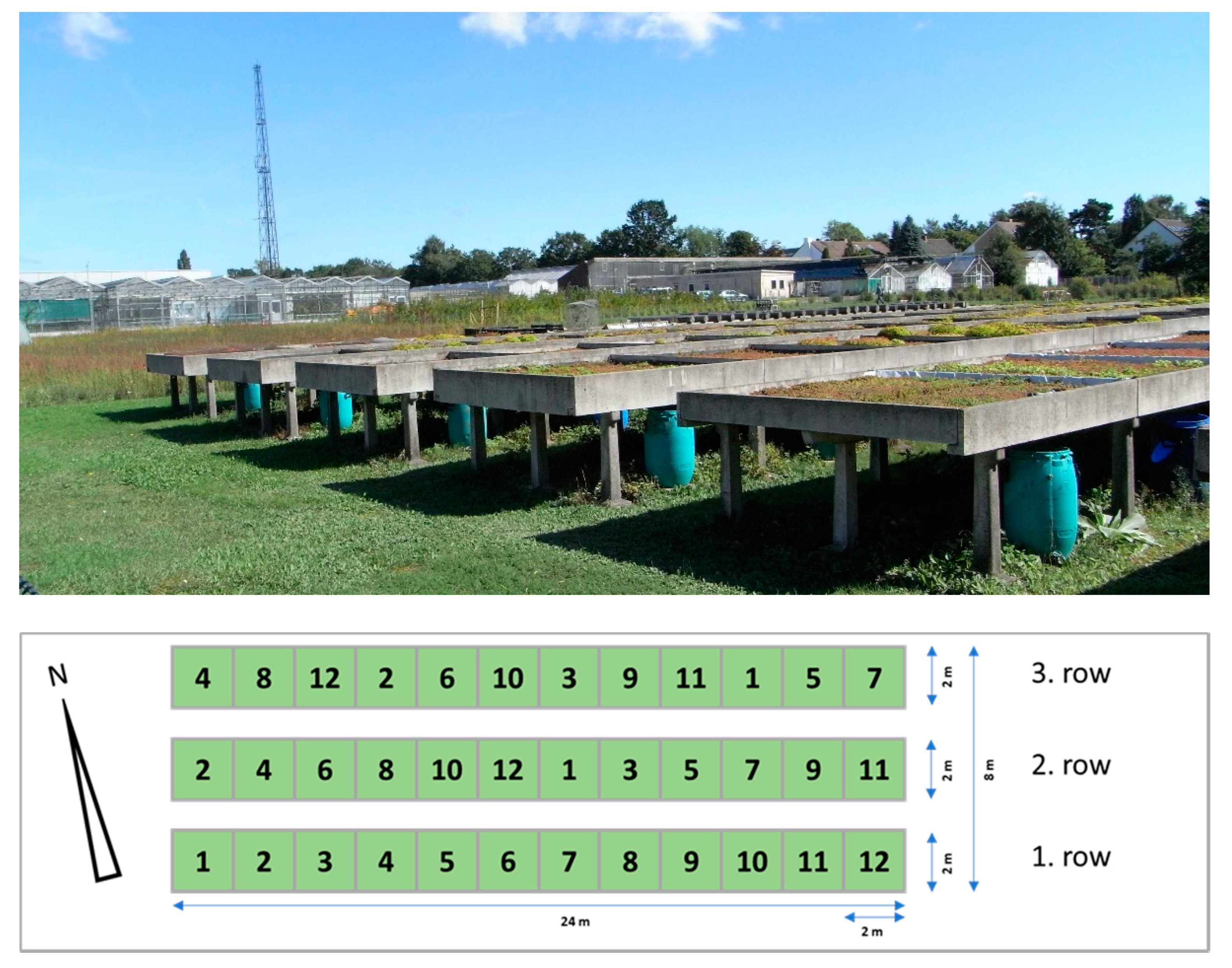
2.1. Field Campaign

The field campaign served to comprehensively examine some roof greening systems, their production, material use and optimization as well as the effects of the different material arrangements (construction methods) on perennial plant development. The product properties were tested in the laboratory. In the following, the most important results of the entire study are summarized, because they have not been published in this form so far. This makes it possible for later simulations to be carried out with other models that can process further parameters. Details can be found in the Supplementary Materials. Furthermore, the daily runoff measurements are available online (see data availability) just as the meteorological data (www.muk.uni-hannover.de/258.html). For the simulations in this paper, only some parts of the original studies were used (e.g., water storage, daily runoff volumes). From 12 construction methods number #10 was not considered in the simulations because it was tested as a special construction method and was not designed with conventional roof greening substrate according to the FLL (Forschungsgesellschaft Landschaftsentwicklung Landschaftsbau e.V.) Roof Greening Guidelines [25].

The field campaign was carried out from July 2002 to the end of August 2006, to determine the vegetation characteristics and the average annual runoff coefficients of thin-layer green roof structures. The campaign was led by Professor Dr. Hans Joachim Liesecke (†) in Hanover-Herrenhausen, at the Institute for Landscape Architecture, at the Department of technical-constructive basics of open space planning (Professor Dipl. Ing. Gilbert Lösken). The campaign examined the properties of the materials used, load assumptions and water storage of the construction methods, the development of the vegetation, the annual water retention and the determination of annual runoff figures. Results compiled up until 2004 have been published by Liesecke [26,27].

The average temperature in Hannover-Herrenhausen is 10.3 °C and the average amounts to 636 mm a⁻¹. The climate corresponds to the cfb climates according to the Köppen–Geiger climate classification [28], i.e., warm-temperate humid climates with cool seasons with mean temperatures of the coldest month between +18° and −3 °C and the mean temperature of the warmest summer month is below 22 °C (summer-warm climates).

The field campaign involved a total of 12 superstructures in triple repetition (Figure 1 and Supplementary Figure S1). The individual test plots were 2 m × 2 m with a slope of 2% and a drainage opening in the middle of the lowest point of the slope. The outflowing water was collected in non-weighable lysimeters (rain barrels) that were read and emptied at 8 A.M. every day. On weekends, readings were taken the following workday.

The rain barrels have a readable, transparent plastic tube on the outside that indicates the water level (principle "communicating tube") as shown in Figure 2. They were previously calibrated in the laboratory. The marks corresponding to 1 liter filling level, approx. 0.25 mm per 4 m² test field. The maximum capacity is 17 mm, i.e., 68 liters. Further runoff leads to overflowing of the rain barrels. For maintenance, a build-up-saturating irrigation and a partial moistening in an initial dry period (2002–2003) as well as an annual fertilization with 30 g m⁻² of a complex long-term fertilizer were administered. Therefore, the undisturbed period from 2004 to 2005 was chosen for the modelling experiments in this study.

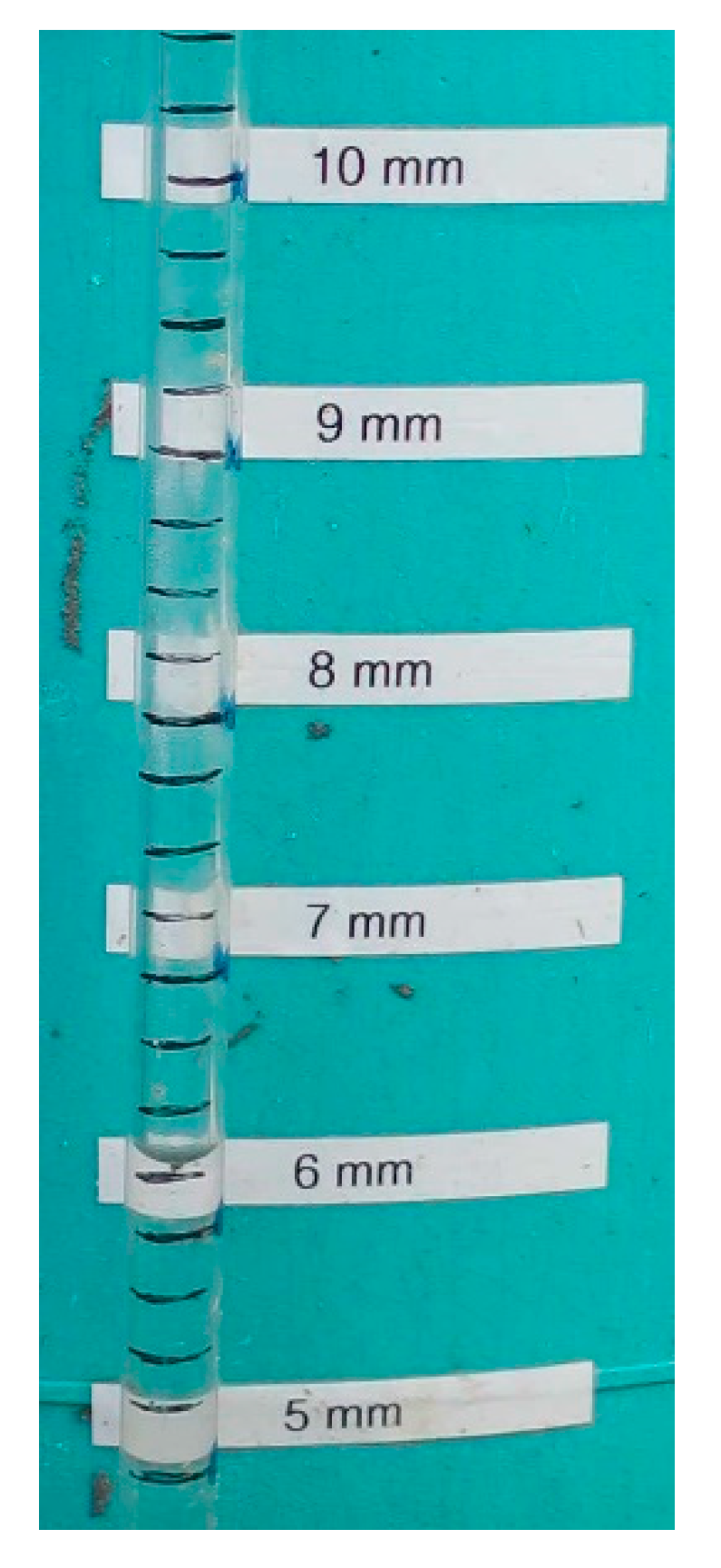
2.1.1. Laboratory Tests

For the substrates used, the grain size distribution, volume weight, maximum water capacity, total pore volume, air volume at maximum water capacity and at pF 1.8, pH, organic material, carbonate content and salt content were determined (Supplementary Table S1–Table S7 and Figure S2). The investigations of the vegetation mats, the protection, storage and drainage mats were carried out on three sections of 40 cm × 40 cm each and the results were extrapolated to 1 m².

Supplementary Tables S8 and S9 summarize the materials used, the respective thickness, the load assumptions dry and at maximum water capacity, as well as the water storage capacity of the construction methods. Due to the thickness and fine-grained composition of the substrate, the vegetation mat has a relatively high water storage capacity. With fleeces, water storage increases significantly while increasing thickness and dry weight. In relation to their thickness, both storage fleeces have a considerably higher water storage capacity than the vegetation mat. The water storage of the drainage and filter mat is very low and insignificant due to its function and structure. In the present order, the thickness of the structure increases essentially from about 3 cm to about 10 cm, which, with some deviations, also results in higher load assumptions and higher water storage.

2.1.2. Perennial Plant Development

For the vegetation surveys, the results of three replicates were averaged. Classification days were at the time of budburst (May), main flowering (July) and retraction (September) in each year. The results of the thirteen classification days of the total vegetation coverage and the coverage share of the vegetation groups, carried out in the years 2002 to 2006, are summarized in Supplementary Tables S10–S12. The development of the vegetation that occurred in the test year 2004 (examples are shown in Supplementary Figure S3) stabilized in the years 2005 and 2006. Except for variants 1 and 2, which have gaps and a total coverage of 90%, it is complete for all variants. The total cover is determined exclusively by the succulents (except variant #1). In summary, the transformation of the herb aspect present at the beginning of the experiment into a sedum-determined aspect was completed by 2006.

Although Sedum album has become the dominant species, the visual aspect is significantly influenced by the variety of other species with different structure and growth height. Supplementary Tables S13 and S14 compare the results obtained for the five Sedum types during the classification days in July and for the experimental years 2002 to 2006. This shows that the intended transformation of the Sedum stand with herbs into a Sedum stand was already achieved after one year and the further development took place in the Sedum group (see Supplementary Tables S13 and S14). The goal to set the foundation for a permanent Sedum population by cultivating the vegetation mat was achieved. The intensity of rooting, the stock density and the shear strength were enhanced by the addition of herbs. While the herbs decreased or completely disappeared after placing the vegetation mat, further development towards a fully developed Sedum population started. This completed development, suggesting a constant vegetation layer, is important for the modelling experiment of the current study, in order to avoid transient vegetation characteristics throughout the simulation period.

2.1.3. Runoff

The runoff was recorded in the period from August 16, 2002 to August 31, 2006. In winter, when temperatures reached freezing point and below, measurements were interrupted, in order to avoid damaging the measuring equipment by ice formation. The downtimes were excluded from further analyses. Based on the precipitation measurements, determined by the nearby meteorological measuring station Hannover-Herrenhausen, operated by the Institute of Meteorology and Climatology (approx. 200 m distance from the study site) and the recorded runoff quantities, the percentage of water retention and the annual runoff coefficient were determined (see

Table A1. Construction technique and material description (including thickness of each substrate, total thickness and water retention) for the different green roof variants and runoff coefficients obtained.

Variant	Construction Technique and Material Description	Thickness (cm)	Water Retention (%)				Runoff Coefficient
			Summer Period	Cooler Period	Winter Period	Average Over Time
1	Vegetation mat	2.5	61.3	42.3	10.4	44.8	0.55
	Protection fleece 300 g m−2
	Geotextile recycling	0.2
		2.7
2	Vegetation mat	2.5	58.3	41.9	7.6	42.4	0.58
	Drainage and filtration mat
	Netting with filtration fleece	1.5
		4.0
3	Vegetation mat	2.5	64.9	47.4	7.6	47.1	0.53
	Water retention mat 800 g m−2
	Geotextile recycling	0.6
		3.1
4	Vegetation mat	2.5	68.9	49.1	11.5	50.6	0.49
	Water retention mat 1200 g m−2
	Geotextile recycling	0.8
		3.3
5	Vegetation mat	2.5	66.1	47.9	10.1	48.5	0.51
	Water retention mat 800 g m−2	0.6
	Drainage and filtration mat
	Netting with filtration fleece	1.5
		4.6
6	Vegetation mat	2.5	68.1	48.2	9.5	49.5	0.51
	Water retention mat 1200 g m−2	0.8
	Drainage and filtration mat
	Netting with filtration fleece	1.5
		4.8
7	Vegetation mat	2.5	71.7	46.3	7.8	50.6	0.49
	Single-layer substrate light
	Pumice 2/8 mm	4.0
	Protection fleece 300 g m−2
	Geotextile recycling	0.2
		6.7
8	Vegetation mat	2.5	69.9	44.7	9.2	49.6	0.50
	Single-layer substrate light
	Expanded clay 2/10 mm	4.0
	Protection fleece 300 g m−2
	Geotextile recycling	0.2
		6.7
9	Vegetation mat	2.5	67.1	44.4	5.7	47.2	0.53
	Single-layer substrate light
	lava 2/8 mm	4.0
	Protection fleece 300 g m−2
	Geotextile recycling	0.2
		6.7
10	Vegetation mat	2.5	61.3	41.1	6.7	43.6	0.56
	Gravel course
	Granulation 16/32 mm	5.0
	Protection fleece 300 g m−2
	Geotextile recycling	0.2
		7.7
11	Vegetation mat	2.5	63.4	41.9	4.7	44.4	0.56
	Multi-layer substrate
	Lava with dolomite and organic matter	3.0
	Drainage and filtration mat
	Netting with filtration fleece	1.5
		7.0
12	Vegetation mat	2.5	67.3	43.7	4.7	46.9	0.53
	Multi-layer substrate
	Lava with dolomite and organic matter	6.0
	Drainage and filtration mat
	Netting with filtration fleece	1.5
		10.0

in the Appendix A). To illustrate the influence of weather conditions, the percentage of water retention for different seasons can be summarized as follows:

• Summer period (from 1st of May to 30th of Sep) between 58% and 72%, subject to a decrease by 1/3 in cooler weather in
• Spring/autumn (from 16th of Mar to 30th of Apr and 01st of Oct to 15th of Nov) between 41% and 49%.
• Winter (from 16th of Nov to 15th of Mar) between 5% and 12%

On average, over the year, a water retention of between 42% and 51% was determined.

2.2. Model Setup

2.2.1. Water Balance Simulation

In order to predict the water balance of green roofs, the Storm Water Management Model EPA SWMM (version 5.1.014) [29] software was used. This model, which is open-source and freely available, is a rainfall-runoff model, widely used to simulate and estimate the hydrological response of urban areas. The LID editor implemented in EPA SWMM makes it possible to define different horizontal layers for green infrastructure and nature-based solutions (NBS) in a sub-catchment. The aim of implementing these tools is to infiltrate, store and evaporate rainwater runoff close to the source, at the expense of runoff. The module “green roof” makes it possible to describe infiltration and evaporation from green roofs in the model. In terms of their area, green roofs are represented as a fraction of their sub-catchments. The empirical Hargreaves approach is the standard method in EPA SWMM to compute ET, based on temperature recordings. It is expressed by the following formula and gives ET₀ in mm d⁻¹ [30]:

$$E{T}_O=0.0023R_a\left(TC+17.8\right){\left(T_{max}-T_{min}\right)}^{0.5}$$

(1)

where $R_a$ is the theoretical maximum extraterrestrial radiation for the considered day of year (mm d⁻¹), $\mathrm{TC}$ is the mean daily temperature (7-day running average) [°C], $T_{max}$ and $T_{min}$ are the maximum and minimum daily temperatures (°C), respectively. This representation of the Hargreaves model (Equation (1)) has fixed parameters, which cannot be modified by the user.

Since this approach does not provide any vegetation-specific parameterization, this study employs a different approach.

2.2.2. Physically-Based ET Simulation

The Penman–Monteith approach describes the diffusion of energy by sensible and latent heat in a network of resistances. It is derived from first principles considering the radiation balance and energy balance of the surface, and therefore it is a physically-based ET model. The Penman–Monteith equation can be written in terms of the latent heat flux LE (W m⁻²) [31]:

$$LE=\frac{∆\left(R_n-G\right)+\frac{{\rho }_a{c}_p}{r_a}\left(e_s-e\right)t_i}{∆+\gamma \left(1+\frac{r_s}{r_a}\right)}$$

(2)

where $∆$ is the slope of the saturation vapor–pressure curve (hPa °C⁻¹), $R_n$ is the net radiation (KJ m⁻² d⁻¹), $G$ is the soil heat flux (KJ m⁻² d⁻¹), ${\rho }_a$ is the mean air density at constant pressure (kg m⁻³), $c_p$ is the specific heat of air (KJ kg⁻¹ °C⁻¹), $e_s-e$ is the vapor-pressure deficit (kPa), $\gamma$ is the psychometric constant (hPa °C⁻¹), $r_a$ is the aerodynamic resistance (s m⁻¹), $r_s$ is the bulk surface resistance (s m⁻¹) and $t_i$ the number of seconds within a time step (daily in this case) [31].

Because it is a physically-based approach, the climatological boundary conditions (i.e., time series of temperature, humidity, wind speed and downwelling shortwave radiation) and vegetation parameters have to be known and understood. Evaporation, using the Penman–Monteith approach, is calculated externally using the open source Python tool “PyETo” [32]. This includes a standardized formula from Allen et al. [33] for ET, from short grass as reference (i.e., the crop reference ET). In this study, the simplified formula for the crop reference ET is adopted, in order to allow adjustments to individual parameters that are fixed in case of the crop reference ET. This, in turn, enables a tailored parameterization of different types of vegetation. In this context, the surface resistance is an important plant parameter that governs ET. It is the resistance of vapor flow from within plant leaves and from beneath the soil surface. It includes both the canopy (leaf area index) and the stomatal resistance, which describes the average resistance of an individual leaf. This resistance is crop specific and differs among crop varieties and crop management.

Combined with the weather data from the test site, suitable ET time series are calculated for arbitrary values of surface resistance [33].

2.2.3. Coupled Modelling Approach

For the simulation, hourly recordings of precipitation are used to force EPA SWMM (Section 2.2.1). As EPA SWMM requires daily values for ET, the calculated ET, using the Penman–Monteith approach (Section 2.2.2) was introduced as an external daily time series. The results obtained from the simulations are aggregated to achieve daily totals, in order to make them comparable with the daily observations of runoff. As a final step, a comparison between simulated and observed runoff is performed to estimate the predictive skill of the calibration schemes. The adjustable parameters that were used to perform the initial model runs are listed in

Table A2. Summary of the final parameter values used in each model run for green roof variants #6. Parameters in italics are subject to automatic calibration in this study. The remaining parameters have been defined a priori.

			Default	Calibrated	Hargreaves	Sensitivity
	NSE (Nash Sutcliffe Efficiency)		0.72	0.85	−0.19	0.83
	PBIAS (Percent Bias)		−37.15	6.15	−125.33	−14.87
	RMSE (Root-mean-square deviation)		1.58	1.18	3.28	1.22
	KGE (Kling Gupta Efficiency)		0.57	0.88	−0.35	0.79
	R (Correlation coefficient)		0.91	0.93	0.73	0.94
Surface	Berm height	(mm)	0	28.46	0.03	17.89
	Vegetation volume	(-)	0.15	0.2	0.1	0.2
	Surface Roughness	(-)	0.15	0.19	0.08	0.19
	Surface slope	(%)	2	2	2	2
Soil	Thickness	(mm)	33	33	33	33
	Porosity	(-)	0.456	0.42	0.42	0.51
	Field capacity	(-)	0.35	0.3	0.24	0.3
	Wilting point	(-)	0.06	0.08	0.12	0.08
	Conductivity	(mm hr−1)	27.6	131.62	65.99	131.62
	Conductivity slope	(-)	5	41.83	24.19	41.83
	Suction head	(mm)	3	30.36	24.54	30.36
Drain	Thickness	(-)	15	15	15	15
	Void fraction	(-)	0.456	0.16	0.17	0.51
	Roughness	(mm)	0.02	0.17	0.27	0.17
FAO	Albedo	(-)	0.20	0.20	0.20	0.20
	Wind exp.	(-)	0.5	0.5	0.5	0.5
	Crop height	(m)	0.12	0.12	0.12	0.12
	rs	(s m−1)	170	78	-	78

in the Appendix A (under column “default”). The properties of the coupled model set up are described in

Table 1. Setup of the coupled EPA stormwater management model (SWMM) model.

Property	Set up
Sub-catchment	A sub-catchment represents a roof of 4 m2 (0.0004 ha) that is 100% impermeable (covered with PVC sheets; N-Imperv PVC: 0.01 [34]), has a slope of 2% and drains entirely to an outfall. It is covered by different low impact development (LIDs) (green roofs).
LID	The sub-catchment is covered by the LID type “Green Roof”. Different LID controls represent the different structures of the test setups. As long as the parameters are unknown, they were estimated and calibrated.
Precipitation	Hourly precipitation data are available. The data for the calibration period (28 Mar 2004–20 Dec 2004) have the following characteristics (Assuming a day from 8 A.M. to 8 A.M. (as observations were sampled at this time each day)): ● Total precipitation: 517.0 mm ● Number of days with precipitation: 153 ● Day with largest precipitation event: 25.29 mm on 7 May 2004
Evapotranspiration (ET)	The Penman–Monteith approach is applied to calculate daily evapotranspiration rates. The data were introduced as external time series to EPA SWMM. The daily evaporation data for the calibration period (28 Mar 2004–20 Dec 2004) has the following characteristics (Using the Penman–Monteith approach, assuming a surface resistance of 78 s m−1): ●  Total evapotranspiration: 321.65 mm ● Number of days with evapotranspiration: 266 ● Day with largest evapotranspiration rate: 4.95 mm on 10 Aug 2004

:

2.3. Calibration and Validation

Since various parameters in the coupled modelling approach are unknown, they are subject to the calibration approach described below. To determine the accuracy of the model outside the calibration period, an independent validation is also considered, following a split sample test [35]:

• Calibration period: 28 Mar 2004–20 December 2004
• Validation period: 22 April 2005–25 November 2005 (due to missing weather data, 2006 was excluded from the analysis)

As shown in

Table 2. Season summaries for the calibration and validation period.

Criteria	Calibration Period	Validation Period
∑ Precipitation (mm)	517.0	388.4
Av. precipitation/d (mm)	1.93	1.79
# Days with prec. > 10 mm d−1 (-)	13	8
# Days with prec. > 20 mm d−1 (-)	3	2
Longest dry period(# days with 0 mm d−1) (d)	12	7
Av. temperature (°C)	12.9	14.8
Max. temperature (°C)	31.4	33.8
Av. ET (mm d−1)	1.2	1.16
∑ ET (mm)	231.65	251.3
Max. ET (mm d−1)	4.95	4.35

both periods differ in terms of weather: the first season (calibration) has a lower average temperature and a higher rainfall total compared to the second season (validation). Thus, ET is higher in the validation period.

The current research employs the open source Python tool spotpy [36] for model calibration. It is a statistical parameter optimization tool that can be used for calibration, uncertainty and sensitivity analysis. In order to customize spotpy to any arbitrary hydrological model, it is necessary to develop an interface to the externally used model. The interface for SWMM was adopted from [37] in order to read different files of ET, based on the sampled resistance values. In addition, the hourly simulated runoff is aggregated to daily data (daily totals from 8 A.M. to 8 A.M. of the subsequent day) after each iteration of spotpy, as observation data are provided in daily resolution.

The Shuffled Complex Evolution (SCE-UA) global optimization algorithm [38] is used in this study. It was found to be a robust algorithm for hydrological model calibration and is widely used in hydrological applications [39]. As an objective function, the Kling–Gupta model efficiency (KGE) is employed [40]. A wise use of the objective function is important because of its high sensitivity. For this case, the KGE seems to be a robust function, as it considers different types of model errors (error in the mean, the variability, and the dynamics) [41]. In addition to KGE, the Nash–Sutcliffe Efficiency NSE [42] and the root mean square error (RMSE) are also computed for each run. The simulated results are compared to the mean of observed values. For all performance measures, days without observations (e.g., weekends) were dropped and those with a runoff higher than 17 mm (This applies to 7th and 10th of May 2004) were set to 17 mm as this was the measurement limit (i.e., the capacity of the rain barrels that collect the runoff). This modification for computing the objective function (i.e., KGE) is necessary to give less emphasis on uncertain peak values in the calibration scheme. However, all display items in this paper (see, Section 3) show the original time series of the model without this modification.

Table A2 in the Appendix A lists all parameters that have been adjusted in the framework of the calibration procedure. Special emphasis is put on the surface resistance, since we intend to find a robust parametrization valid for all test sites, which show the same vegetation characteristics. This is motivated by the fact that, despite the different structures, the different green roof variants underwent a similar evolvement of the vegetation coverage as evidenced by the uniform vegetation development in the field campaign (Section 2.1). Hence, it is assumed that vegetation characteristics in our modelling experiments are uniform in space across all test sites. In turn, calibration involves the following steps:

• 1st iteration: Run spotpy, applied to the coupled modelling approach with 5 repetitions for each test plot (to see how the stochastic nature of sampling affects results), in order to find a unique representative surface resistance value. Various evapotranspiration time series are calculated (with a surface resistance range from 60 to 300 s m⁻¹). These files, or more specifically the file path in the EPA SWMM’s input file, are available as adjustable parameters to the calibration scheme. For this purpose, an existing EPA SWMM model driver in spotpy has been adjusted (https://github.com/mmmatthew/swmm_calibration (last access 24 Nov 2020)). This way, the surface resistance is estimated directly as a yearly average, suggesting that a seasonal variation is neglected.
• Based on the results of the previous step, a comparison of surface resistance values across the simulations for all test plots is carried out. An average value out of all surface resistance values is computed, in order to find a unique representative value.
• 2nd iteration: Rerun spotpy calibration with SCE-UA (Shuffled complex evolution method developed at The University of Arizona) for all green roof variants to calibrate the LID parameters in EPA SWMM (surface layer, soil layer, drainage mat), assuming a fixed surface resistance from the previous step. Compute performance measures for the calibration and validation period, respectively.

2.4. Global Sensitivity Analysis

To consider parameters with a high impact on the model results, an additional global sensitivity analysis, also using the Python tool spotpy [36], complements the previous calibration procedure. The algorithm "Extended FAST" based on [43] is selected for this purpose. Besides “Sobol”, this is the only method that takes parameter interaction into account [44]. The method is based on the Fourier amplitude sensitivity test (FAST) and allows quantifying the total contribution of each input factor to the variance of the output to be calculated. These methods are complex and to keep the explanations concise, we will only provide a brief overview of how Extended FAST works in principle. At first, the algorithm creates matrices for parameter sampling [45]. Then a bootstrap technique is applied to the matrices which relies on replacement of elements. Based on that, real model parameters are derived from sampled values and the corresponding model output is then used to calculate the parameter sensitivity [44] based on the estimator proposed by Jansen [46].

The main advantages of “Extended FAST” are its robustness, especially with small sample sizes, and its computational efficiency [43]. Important for this algorithm is the small number of iterations in order to obtain reliable information about the parameters. It can be calculated according to [44]. Finally, the algorithm provides a sensitivity index for each parameter. The sensitivity index is a reliable measure to rank parameters according to their relative importance [44]. Hence, comparing the sensitivity index among all parameters allows for ranking the importance of parameters.

First, the literature (default) values for common value ranges of the EPA SWMM parameters are defined as the initial parameter set (see “default” column in Table A2 in the Appendix A). This parameter set includes those parameters that are adjusted in each iteration of the algorithm and generally unknown (e.g., the conductivity slope). Indeed, known characteristics of the field campaign, e.g., the dimension of each green roof variant and the layer structure remain unchanged during parameter sampling. As a simplification—except for the surface resistance—the Penman–Monteith parameters that describe vegetation characteristics remain fixed (Albedo: 0.2, crop height: 0.12 m, height wind exponent a: 0.5, rs: 78 s m⁻¹). This is assumed to be feasible, since the surface resistance is the most sensitive parameter for plants subject to limited water availability [47], which applies in particular to green roofs. To avoid possible negative impacts arising from the selected value ranges for each parameter, each range is extended by ±20 and ±50%. Since “Extended FAST” also involves KGE as an objective function, it serves as another independent approach for model calibration.

3. Results

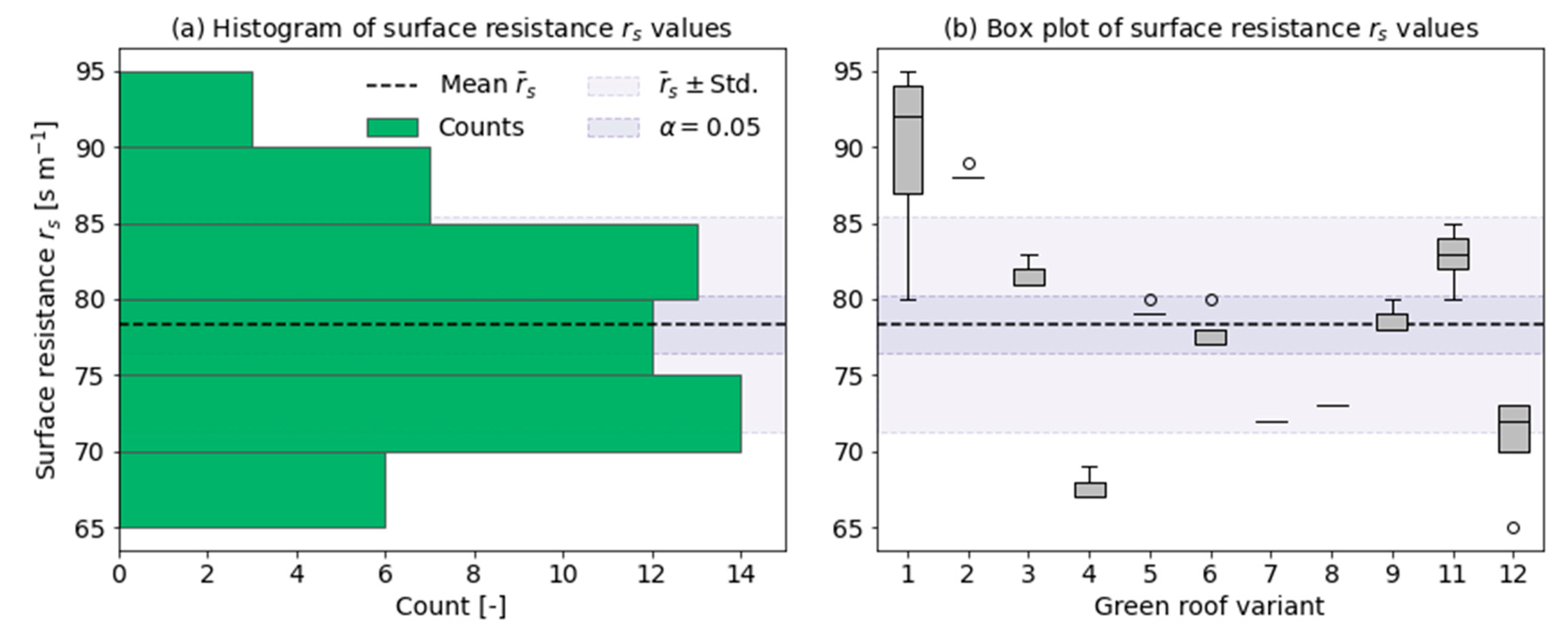
3.1. Representative Surface Resistance

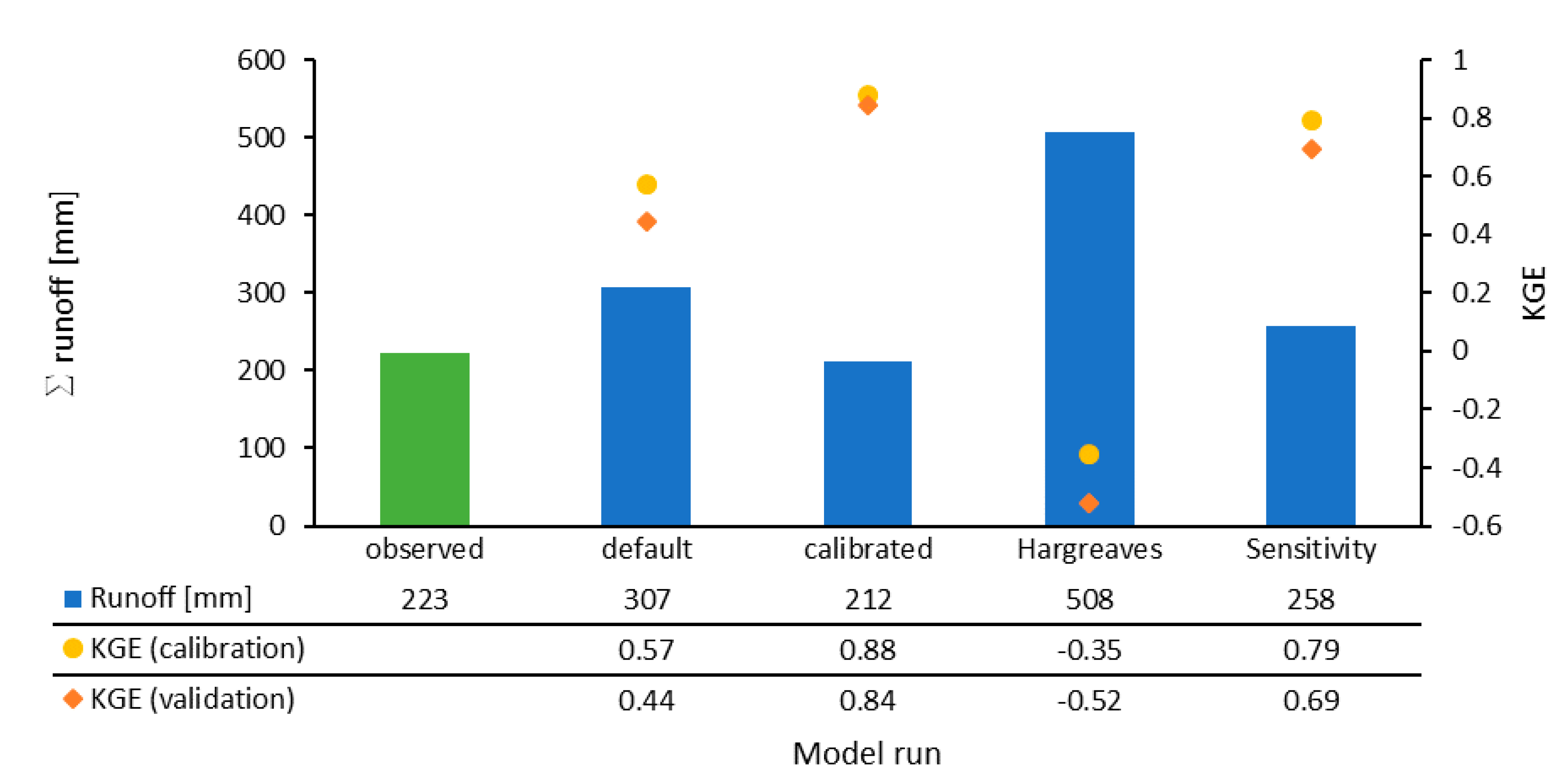
In the first step of the calibration procedure, the identification of a unique, representative value of surface resistance is addressed. The SCE-UA algorithm in spotpy is applied five times to each test site (green roof variant). Figure 3 shows a histogram including all surface resistance values and box plots, visualizing the best estimate of surface resistance for each green roof variant. The results indicate that SCE-UA yields consistent estimates of surface resistance across all test sites. Since we seek to understand surface resistance as a vegetation property, which is assumed to be homogeneous in all experiments, an average value is computed (first iteration) and applied in each following run of SCE-UA algorithm in spotpy (second iteration).

3.2. Model Runs

The surface resistance found to be representative for all test plots is then used as a fixed value in the 2nd iteration of the calibration procedure (see Section 2.3). After recalibration of EPA SWMM for each test plot, assuming a fixed surface resistance of 78 s m⁻¹, the final runs are demonstrated in this section. Test plot #6 is chosen as a reference here, for which we show the detailed results. The corresponding plots for all other test plots are provided in the Supplementary Materials, together with the final parameter values (see Supplementary Figures S5–S24 and Table S17). The validation of the final model and the global sensitivity analysis are presented in Section 3.3 and Section 3.4, respectively. Based on the sensitivity analysis, another model run is performed to test if less sensitive parameters could be neglected whilst achieving acceptable results.

The daily response (i.e., the aggregation of hourly time series to achieve daily time series, which match the time step of observations from 8 A.M. to 8 A.M. of the subsequent day) of the green roofs is plotted for both observed and simulated values. First, the results of the uncalibrated model (model with default parameters) are reviewed as the baseline model. Then, we show the results of the corresponding model that was calibrated with the two iterations of SCE-UA and the fixed surface resistance value of 78 s m⁻¹. The results of a model setup using the Hargreaves method, which is the standard approach implemented in EPA SWMM instead of the Penman–Monteith method, are presented alongside the former, to show the added value of the coupled modelling approach.

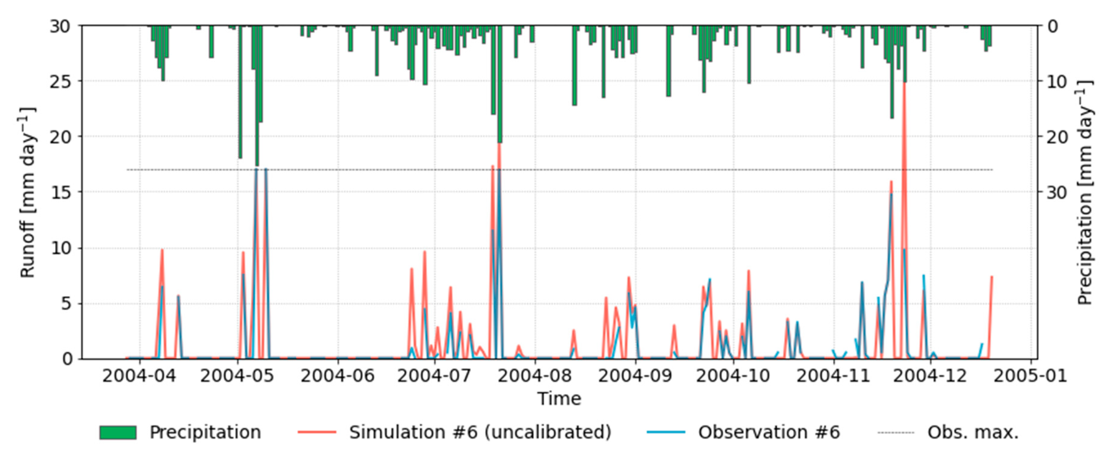
3.2.1. Model Run with Default Parameters

For the uncalibrated model, the default parameter values from the literature review were applied [21,29]. Simulation and observation show similar patterns in terms of timing and variability of the time series, but the simulation overestimates the runoff. Results for green roof variant #6 are visualized in Figure 4. The value for the objective function, more specifically, the Kling–Gupta efficiency (KGE), is 0.57.

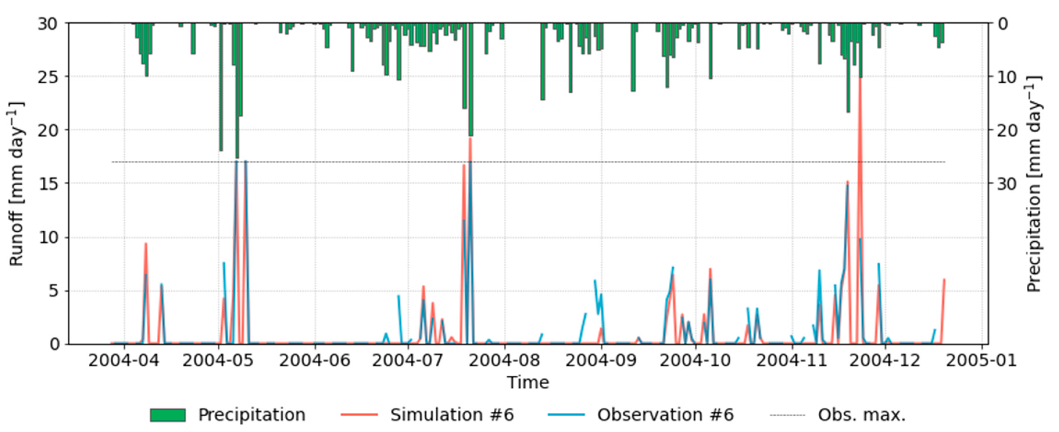
3.2.2. Calibrated Model

For the calibrated model, the calibrated LID parameters for the surface, soil and drainage mat (second iteration) are considered, together with the surface resistance value from the first iteration (Table A2 in the Appendix A). Modelled and observed time series coincide well, even though the simulation sometimes slightly underestimates observed runoff (except for days when observed runoff exceed the capacity of the rain barrel of 17 mm). Results for green roof variant #6 are presented in Figure 5. The Kling–Gupta efficiency (KGE) reaches 0.88, which underlines the added value of calibration, compared to the uncalibrated model (KGE = 0.57).

Figure 6 shows the water balance for the calibrated model setup in terms of mass curves. Both observed and simulated runoff are displayed, as well as the difference between precipitation and evapotranspiration. The results refer to green roof variant #6 and highlight that the calibrated model matches the observed time series very well. Total runoff is satisfactorily represented in the experiment.

The good model performance is also reflected by the statistical summary in

Table 3. Summary of runoff characteristics for green roof variant #6 in calibration and validation period, respectively.

Criteria	Calibration Period	Validation Period
Mean daily runoff (obs #6) (mm d−1)	1.16	0.97
Mean daily runoff (sim #6) (mm d−1)	1.14	0.91
Longest dry period (obs #6) (d)	43	49
Longest dry period (sim #6) (d)	54	59

(first column). Both observed and modeled average runoff compare well. However, the longest dry period (i.e., consecutive days with zero runoff) is overestimated by the model, which is also obvious from comparing the time series in Figure 5. The runoff event in late June 2004 is not reproduced by the model. However, the majority of events is captured well in the simulations.

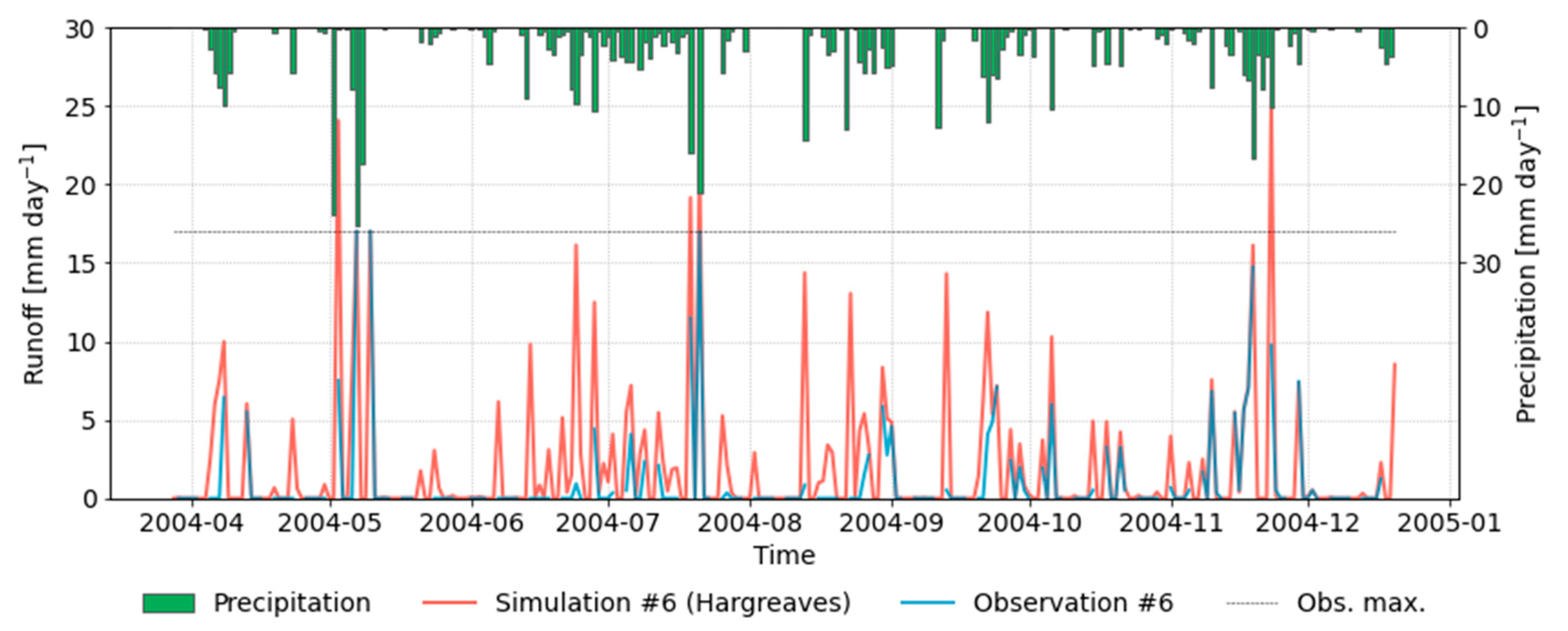
3.2.3. Model with the Integrated Hargreaves Method for ET

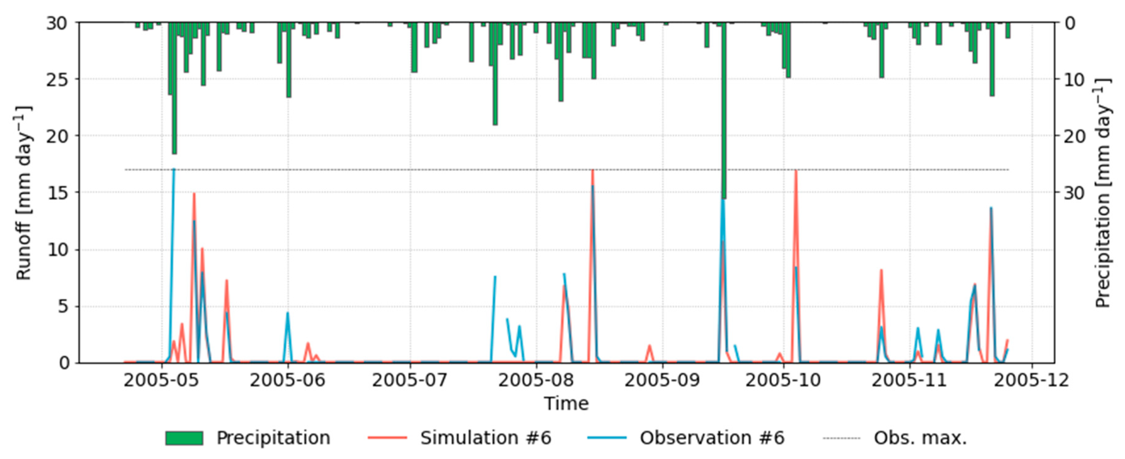
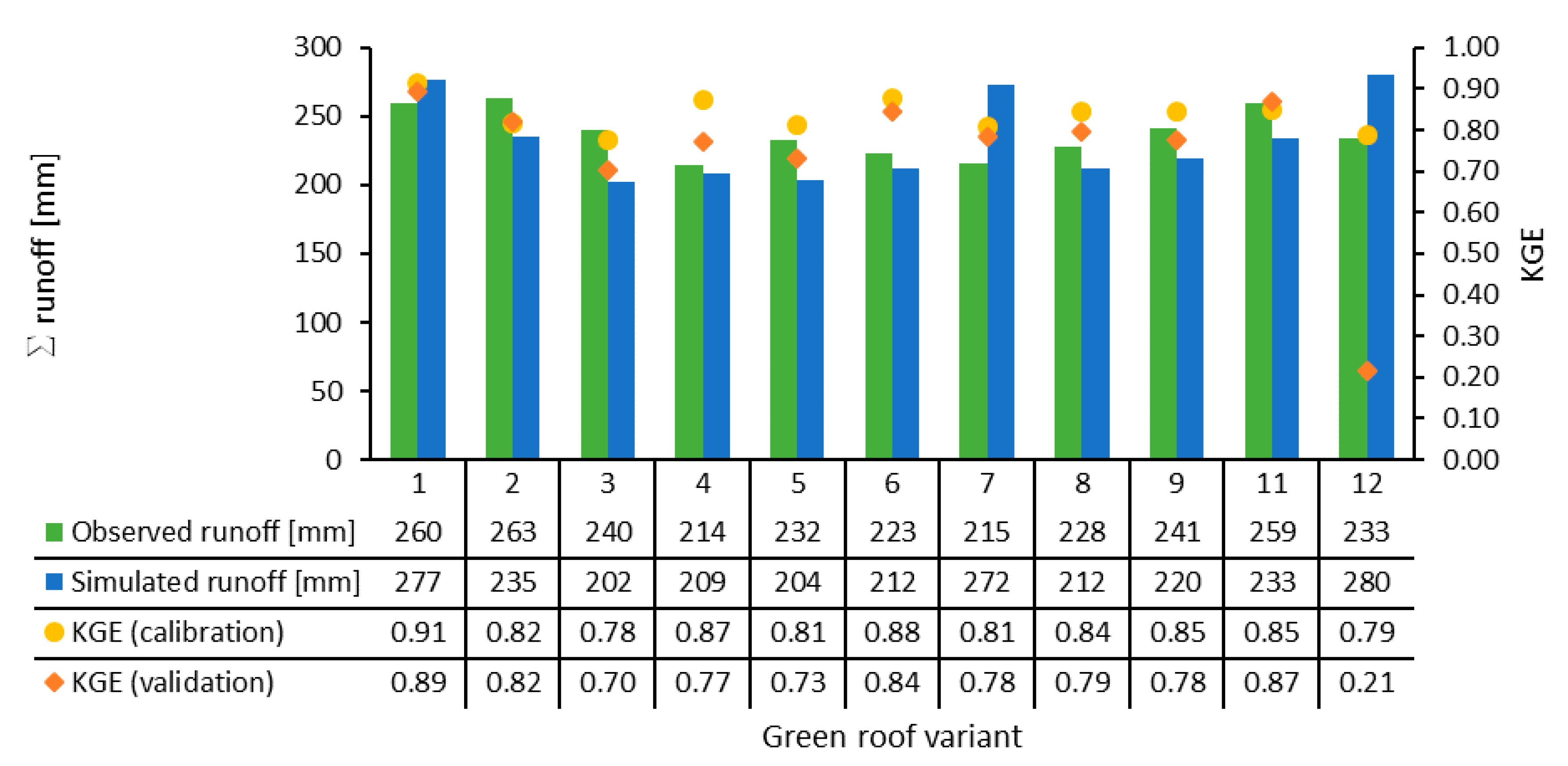
For reasons of comparison, the model was also calibrated and run using the original Hargreaves method, which is already implemented in EPA SWMM. Similar to the previous runs, runoff time series for green roof variant #6, obtained from the EPA SWMM setup with the Hargreaves method, are presented in Figure 7. The simulation does not only overestimate total runoff but also runoff variability. The Kling–Gupta efficiency (KGE) is −0.35, suggesting that the Penman–Monteith approach clearly outperforms the Hargreaves method in case of our test site.

3.3. Validation

The validation of the calibrated model (Section 3.2.2.) shows similar patterns between observation and simulation, but the simulation sometimes underestimates the runoff. Results for green roof variant #6 are presented in Figure 8. The Kling–Gupta efficiency (KGE) is in this case equal to 0.84, which is a value close to the corresponding value achieved for model calibration (KGE = 0.88). Table 3 also confirms that runoff characteristics are presented well by the model, even though the longest dry period is also overestimated in the validation period (the event in late July is not captured by the model). However, it is assumed that the model shows predictive skill outside the calibration period, since the performance measures of the validation period reflect a similar accuracy as those values achieved in the calibration period (Table A2 in the Appendix A)

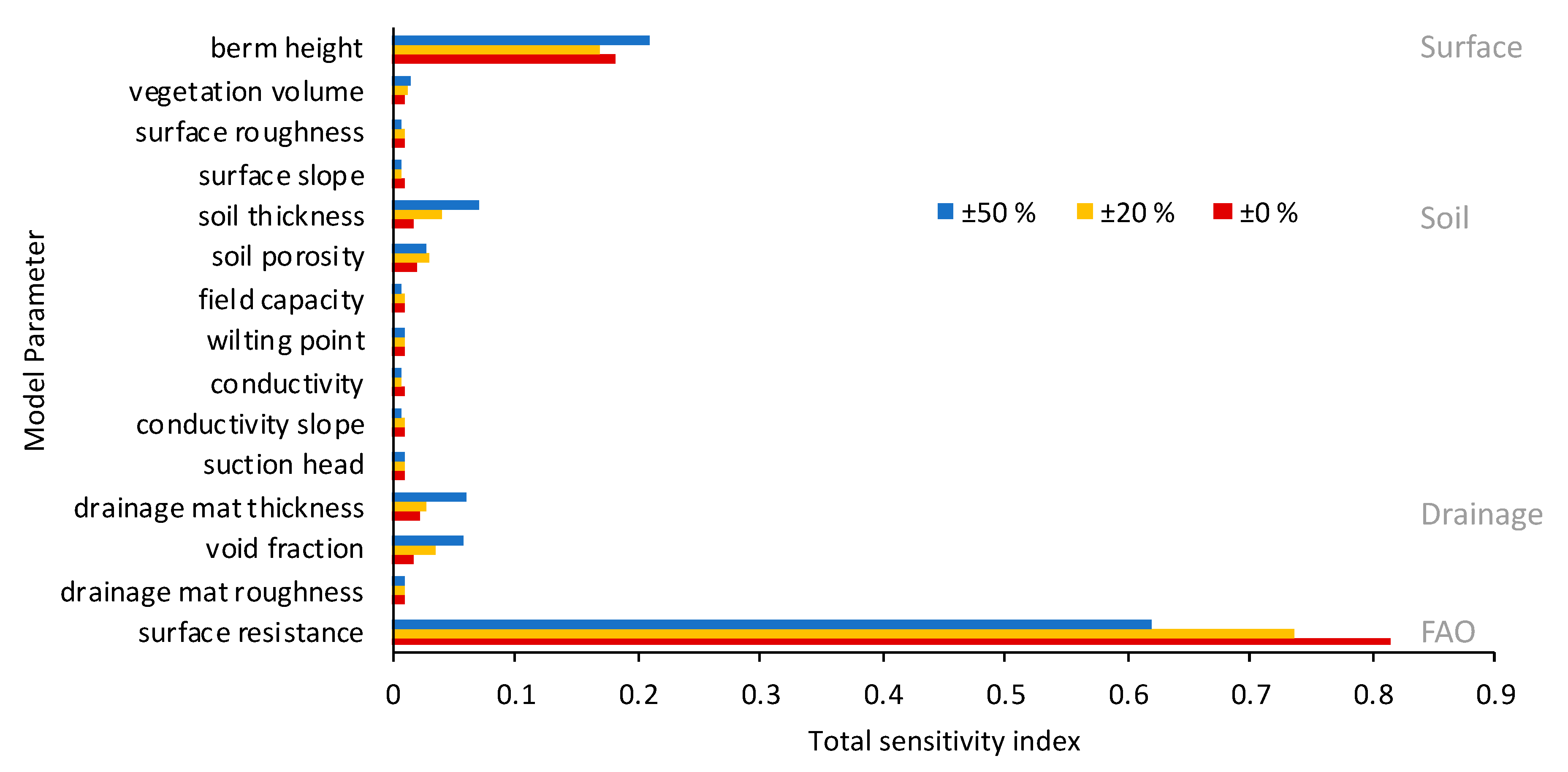
3.4. Global Sensitivity Analysis

The results of the global sensitivity analysis are presented in terms of the total sensitivity index (with a maximum of one, see Section 2.4). According to the sensitivity analysis, the model is most sensitive towards the following parameters: surface resistance and berm height. The computed sensitivity index is smaller for soil thickness, soil porosity, drainage mat thickness, and drainage mat void fraction, indicating that these parameters are less important in our experimental setup (Figure 9).

This allows for re-running the calibration scheme with a smaller number of adjustable parameters. As the soil thickness was given by the field campaign, this value was not calibrated and another simulation is carried out calibrating only the remainder of the most sensitive parameters (i.e., berm height, soil porosity and drainage mat void fraction). The calibrated surface resistance of 78 s m⁻¹ is also used here. By calibrating only these sensitive parameters, the simulation yields a Kling–Gupta Efficiency (KGE) of 0.79 (run not shown here), which is consistent with the calibration utilizing SCE-UA (KGE = 0.88).

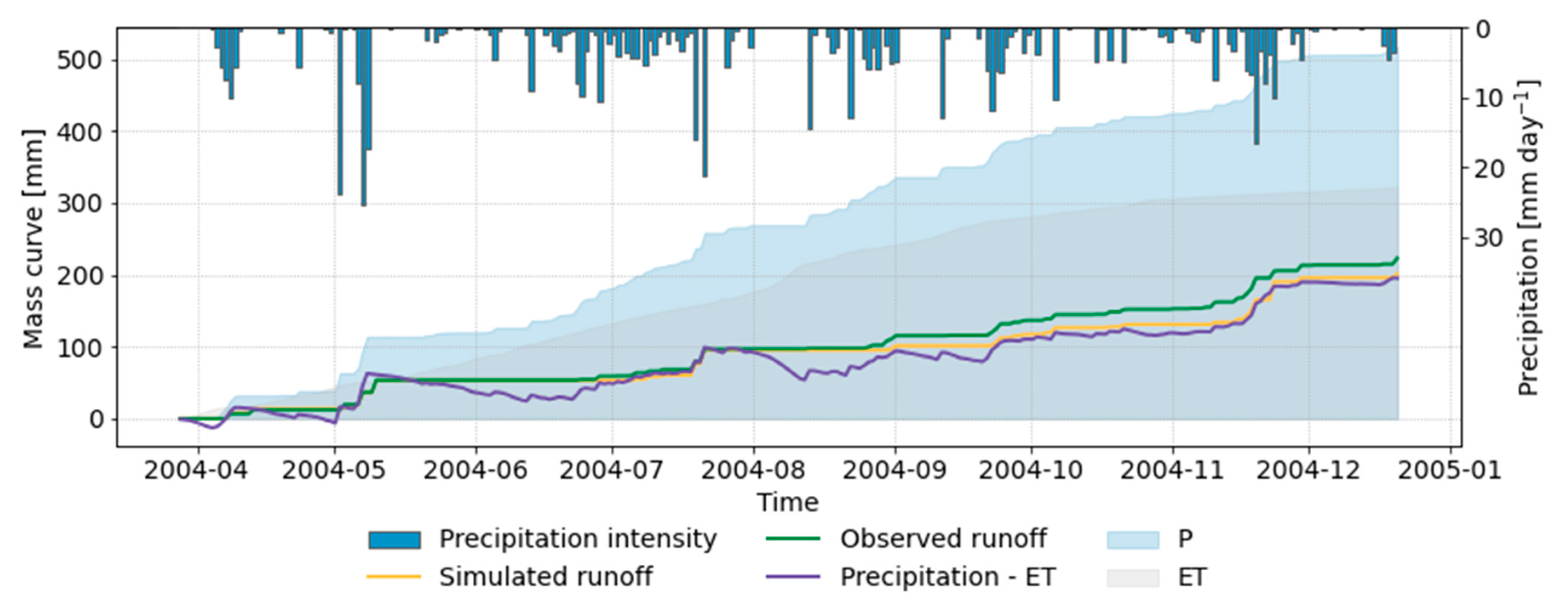
3.5. Synthesis of Model Runs

To summarize the different model runs described previously, the total runoff and the Kling–Gupta efficiencies (KGE) obtained in each model are compiled in Figure 10. Especially when using the Hargreaves method implemented in EPA SWMM, the total runoff is clearly overestimated while ET is underestimated. The calibrated model and the model calibrated with only sensitive parameters (referred to as “sensitivity” run) show the best efficiencies (KGE 0.88 and 0.79), which is confirmed by similar model skill values achieved for the validation period (see Table A2 in the Appendix A). In contrast, the efficiencies using the model with the Hargreaves method are −0.35 and −0.52, for the calibration and validation periods, respectively. This mismatch, expressed by the negative KGE values, is mostly determined by the too low values of ET computed by the Hargreaves method, which in turn exaggerates the hydrological response in terms of runoff, which is more than twice that of the observed value.

While all previous results pertain to green roof variant #6, Figure 11 compiles corresponding metrics for the entire set of eleven green roof variants (see Section 2.1 for reference to the green roof variants). Besides total runoff in the calibration period, the Kling–Gupta efficiencies (KGE) of calibration and validation periods are compiled likewise. The performance measures for all green roof variants are listed in

Table A3. Performance measures for all green roof variants.

	Objective Function	#1	#2	#3	#4	#5	#6	#7	#8	#9	#11	#12
Calibration	NSE	0.87	0.77	0.80	0.85	0.82	0.85	0.88	0.83	0.85	0.87	0.85
	PBIAS	−2.51	14.63	20.15	7.14	16.63	6.15	−13.82	11.33	13.03	13.88	−15.29
	RMSE	1.16	1.57	1.38	1.14	1.31	1.18	1.05	1.23	1.22	1.16	1.20
	KGE	0.91	0.82	0.78	0.87	0.81	0.88	0.81	0.84	0.85	0.85	0.79
	R	0.94	0.89	0.91	0.93	0.92	0.93	0.96	0.93	0.93	0.94	0.94
Validation	NSE	0.84	0.83	0.56	0.63	0.62	0.73	0.77	0.69	0.67	0.82	0.31
	PBIAS	−3.80	14.51	19.61	13.35	18.25	6.16	−13.45	12.73	14.61	9.39	−51.59
	RMSE	1.33	1.44	2.04	1.87	1.92	1.45	1.45	1.69	1.83	1.37	1.84
	KGE	0.89	0.82	0.70	0.77	0.73	0.84	0.78	0.79	0.78	0.87	0.21
	R	0.92	0.91	0.78	0.81	0.80	0.87	0.91	0.84	0.83	0.91	0.90

in the Appendix A. Except for green roof variants #1, #7 and #12, the total runoff is always slightly underestimated (percent bias (PBIAS) = 6% on average (Please note that positive PBIAS values indicate underestimation of the model, while negative values suggest a model overestimating observed values [48].)). On the one hand, this underestimation is acceptable for streamflow simulations (very good performance if PBIAS ≤ ±10% [48]). On the other hand, the model has been calibrated against observed runoff while maximizing KGE, which considers not only the model bias but also the correct timing and magnitude of peaks, thus representing a compromise of several aspects of calibration. In green roof variant #12, however, runoff is overestimated by 20%, in green roof variant #7 by 26%. For all green roof variants, the Kling–Gupta efficiencies (KGE) vary from 0.77 to 0.91 for the calibration period and from 0.7 to 0.89 for the validation period, respectively. Only the KGE for green roof variant #12 is significantly lower with 0.21. It is also noted that the Kling–Gupta efficiencies of calibration and validation periods are similar (with exception of green roof variant #12), which justifies using the calibrated parameters outside the calibration period.

4. Discussion

To investigate an improved representation of the hydrological response of green roofs, a combined model using the Penman–Monteith approach and EPA SWMM was set up. Detailed data from a field campaign served as a basis and the measurements were used to calibrate and validate the model.

A multiple parameter calibration of LID parameters (surface, soil and drainage) shows distinct improvement to the default model using literature values (increase in KGE from 0.57 to 0.88). The calibration of the surface resistance seems to be the best method to take the vegetation feedback into account, since it also helps to improve the representation of the water balance closure of the model, through more representative ET estimates. ET is computed with daily temporal resolution, which is consistent with the expected format of time series and can be used to force EPA SWMM with external ET simulations. The model, however, was integrated using hourly time steps, which is considered a reasonable approach, since EPA SWMM is mostly applied to urban drainage studies that involve sub-daily time steps due to short times of concentration in urban areas [49].

The added value of the coupled model, involving both EPA SWMM and the Penman–Monteith approach, is obvious, given that the uncalibrated model with KGE = 0.57 even outperforms a calibrated EPA SWMM setup with Hargreaves method to compute ET. The latter model, shows a poor model performance due to ET underestimates, yielding negative KGE values. As long as the coefficients of the Hargreaves equations in EPA SWMM cannot be adjusted, it is not possible to calibrate ET simulations in the original approach of EPA SWMM, employing the Hargreaves equation [50]. An external calculation with calibrated coefficients might yield better results, but this goes beyond the scope of the research question, since this study is not about comparing different evapotranspiration methods, but rather about showing an improvement in the modelling of runoff from green roofs with EPA SWMM.

Extreme events and rainfall events after long dry periods are represented with lower accuracy in our modelling experiments. Since the interest of the study is on the vegetation feedback rather than on extreme events, this inaccuracy is accepted here. In addition, observed values are subject to a maximum value of 17 mm per day due to the limited capacity of the rain barrels used to collect runoff from the test plots, rendering the accurate representation of extreme events impossible.

A global sensitivity analysis shows that in case of our modelling experiments, only a few soil parameters are sensitive in EPA SWMM. One of them is the berm height that describes how much water can pond, therefore suggesting an additional storage. The construction thickness and porosity also describe the storage volume. Accordingly, the model reacts in a particularly sensitive way, as a consequence of changing water storage. Other descriptive parameters are less influential and might be neglected in the calibration according to the investigations. Here, we describe the possibility to consider a simplification of the parameterization of EPA SWMM, suggesting a lower number of parameters that need to be adjusted in the calibration procedure. The coupled model is particularly sensitive to the surface resistance. This selected vegetation parameter influences ET significantly and thus governs the simulation of the water balance of green roofs. Due to its high sensitivity, it is recommended to focus on this parameter, especially in cases of different vegetation.

Regarding the parameters analyzed in the framework of the automatic calibration (Table A2 in the Appendix A and Supplementary Table S17), similarities are found among the green roof configurations, which can be related to their characteristics (Supplementary Tables S8 and S9). For instance, the porosity is higher for green roof variants #7, #8, and #9 when compared to green roof variants #1 to #6. This sampling of parameters is feasible, given that the green roof variants #7, #8, and #9 consist of a single-layer substrate with higher porosity than the geotextiles. Likewise, for green roof variants #3 and #5, the drainage mat void fraction is higher than for #1, #2, #4, and #6, which is supported by the construction details (e.g., green roof variants #5 have two drainage layers instead of one). The drainage mat of green roof variants #6, however, shows a much higher density of the material, suggesting that the void fraction is much lower (Supplementary Table S17). All these parameters were found through optimization, suggesting that they are also effective parameters rather than physical constants [51]. For instance, the berm height is a calibrated parameter loosely linked to the physical characteristics and thus representing model uncertainty and scaling issues as well. However, we can identify some groups of green roof variants that show similar parameters (i.e., porosity, field capacity), e.g., green roof variants #1 to #6 with geotextiles, green roof variants #7 to #9 which represent single layer substrates and green roof variants #11 and #12 that are multi-layer substrates, whereby #12 has the highest vertical extent.

The validation for several green roof variants confirms the accuracy of the model, suggesting that it can be applied to other time periods as well as to other green roof variants. Moreover, the results confirm that a unique, representative estimate of the surface resistance parameter highlights that our model setup reflects a robust model parameterization for vegetation, even though we neglect important mechanisms in our model setup, e.g., the CAM metabolism of Sedum and seasonality of surface resistance [22]. Still, an open question refers to the lower model performance found for green roof variant #12 (higher storage). Given that the setup clearly differs from the remaining green roofs, several reasons could in principle hold responsible for this mismatch. To gain insight into this question, another objective function or a different optimization might help to see if better model results are possible when applying EPA SWMM to green roof variant #12. However, this goes beyond the scope of this study.

5. Conclusions

In this research article we present a coupled modelling approach comprising EPA SWMM and PyETo. In this method, the hydrological model EPA SWMM is complemented by a more comprehensive representation of ET, which is computed using the Penman–Monteith approach. Based on numerous green roof test plots, which are represented in the coupled model, we show that:

(i)

the model confirms that shallow layered extensive green roofs show good retention capabilities with a minimum roof load, as witnessed by the lower average value and longer dry spell period observed for runoff (compared to rainfall, see Table 1 and Table 3);

(ii)

the coupled modelling approach outperforms the standard EPA SWMM model with Hargreaves ET computation, even without any further calibration of the ET component;

(iii)

a robust parametrization of the vegetation (or more specifically surface resistance) is possible for different green roof configurations with similar vegetation cover;

(iv)

only a subset of LID parameters in EPA SWMM are sensitive for continuous simulations, namely surface resistance, berm height, soil porosity and the drainage mat void fraction.

Since these findings mostly apply to 11 independent green roof tests sites (three repetitions for each), for which we identified a unique representative surface resistance parameter governing ET, the parameterization of the coupled modelling approach is viewed as being robust in terms of transferability in space (different test plots) and time (independent validation period).

The coupled modeling approach allows for the determination of the water balance components on green roofs by applying a more accurate continuous simulation, which shows major advantages for design flood estimation when compared to event-based approaches [52], for example, by the implicit incorporation of antecedent soil moisture conditions [16]. However, long and continuous rainfall series are not always available and present a low resolution. Thus, stochastic rainfall models could be used in combination with the coupled model to overcome this problem [15,53] and perform continuous simulations in urban hydrology.

However, it is worth mentioning that several uncertainties have so far not been considered. Among other aspects, these include:

(i)

the design of the existing field campaign was not tailored to provide a basis for modelling studies. Hence, hydrological quantities that might complement constraining the model for dry and wet periods, such as soil moisture measurements, have not been addressed;

(ii)

The non-stationarity of vegetation characteristics was not considered in our study. For instance, Sedum tends to recover within one week after drought stress [54]. Moreover, surface resistance might undergo seasonal changes and might be subject to changes as a response to drought stress, as idealized irrigation experiments after drought might suggest [55];

(iii)

Equifinality (i.e., different parameter sets yield similar results or accuracy in terms of objective function) is still a source of uncertainty in studies aimed at parameter identification [56]. Some parameters are effective parameters, suggesting that their original physical meaning is not always given due to model uncertainty and scaling issues [51].

However, since the field campaign comprises three independent samples for each green roof configuration—the differences between which are small (working with an average for each configuration is feasible)—our results are considered robust in terms of parameterization. Even though some uncertainties arise from the limit of 17 mm per day, reflecting the maximum runoff observed on a specific day, there is only limited evidence on the predictive skill for extreme events, especially since rainfall observations from the weather station are also subject to uncertainties.

Apart from these limitations, our coupled model setup is a substantial step forward in modelling green roofs in urban drainage studies, especially since the components involved here (EPA SWMM, PyETo, and spotpy) are available free of charge and coupling the models is straightforward—without the need to modify the EPA SWMM code—as it is possible to force the model with external ET files. The full set of meteorological quantities needed to utilize Penman–Monteith (instead of temperature only) is also available from re-analysis data, e.g., ERA5 (European Centre for Medium-Range Weather Forecasts. European Reanalysis 5), making it possible to drive the coupled modelling approach for arbitrary sites. Even with limited information on the detailed characteristics of the green roof, we demonstrate that the coupled modelling, even without any further calibration, is capable of outperforming the original EPA SWMM ET simulation, based on the Hargreaves equations. Moreover, some practical recommendations on constraining the number of adjustable parameters are given.

As an outlook for future research, it is recommended to better address the non-stationarity of vegetation characteristics of green roofs. In the present study, we demonstrate that the assumption of a constant surface resistance value across different green roof variants with similar vegetation coverage is valid. This is an important finding, since the surface resistance is hence transferable in space. However, a seasonally varying surface resistance value might help to better predict season onsets and drought stress recovery (e.g., by involving weather data to adjust parameters depending on the season [57]). Thus, a time-varying parameterization might complement the spatially uniform parameterization of vegetation across the test sites. In addition to a constant surface resistance applied to all sites (as studied here), a uniform method that describes the temporal variation of the surface resistance parameter should be investigated in the future.

For the design of field campaigns for green roofs, we also recommend sampling hydrological quantities other than runoff, to better constrain the parameter optimization of the hydrological model, through employing a multi-objective calibration. Moreover, field campaigns with similar characteristics should be carried out in different climate zones, to investigate the effect of climate on parameter optimization.

References

1. Mentens, J.; Raes, D.; Hermy, M. Green roofs as a tool for solving the rainwater runoff problem in the urbanized 21st century? Landsc. Urban Plan. 2006, 77, 217–226. [Google Scholar] [CrossRef]
2. Milly, P.C.D.; Wetherald, R.T.; Dunne, K.A.; Delworth, T.L. Increasing risk of great floods in a changing climate. Nature 2002, 415, 514–517. [Google Scholar] [CrossRef]
3. Shafique, M.; Kim, R. Low Impact Development Practices: A Review of Current Research and Recommendations for Future Directions. Ecol. Chem. Eng. S 2015, 22, 543–563. [Google Scholar] [CrossRef] [Green Version]
4. Alfredo, K.; Montalto, F.; Goldstein, A. Observed and Modeled Performances of Prototype Green Roof Test Plots Subjected to Simulated Low- and High-Intensity Precipitations in a Laboratory Experiment. J. Hydrol. Eng. 2010, 15, 444–457. [Google Scholar] [CrossRef]
5. She, N.; Pang, J. Physically Based Green Roof Model. J. Hydrol. Eng. 2010, 15, 458–464. [Google Scholar] [CrossRef]
6. Carson, T.B.; Marasco, D.E.; Culligan, P.J.; McGillis, W.R. Hydrological performance of extensive green roofs in New York City: Observations and multi-year modeling of three full-scale systems. Environ. Res. Lett. 2013, 8, 24036. [Google Scholar] [CrossRef]
7. Bolliger, J.; Silbernagel, J. Contribution of Connectivity Assessments to Green Infrastructure (GI). IJGI Int. J. Geo-Information 2020, 9, 212. [Google Scholar] [CrossRef] [Green Version]
8. Oberndorfer, E.; Lundholm, J.; Bass, B.; Coffman, R.R.; Doshi, H.; Dunnett, N.; Gaffin, S.; Köhler, M.; Liu, K.K.Y.; Rowe, B. Green Roofs as Urban Ecosystems: Ecological Structures, Functions, and Services. BioScience 2007, 57, 823–833. [Google Scholar] [CrossRef]
9. van Mechelen, C.; Dutoit, T.; Hermy, M. Adapting green roof irrigation practices for a sustainable future: A review. Sustain. Cities Soc. 2015, 19, 74–90. [Google Scholar] [CrossRef]
10. Cascone, S.; Coma, J.; Gagliano, A.; Pérez, G. The evapotranspiration process in green roofs: A review. Build. Environ. 2019, 147, 337–355. [Google Scholar] [CrossRef]
11. Li, Y.; Babcock, R.W. Green roof hydrologic performance and modeling: A review. Water Sci. Technol. 2014, 69, 727–738. [Google Scholar] [CrossRef] [PubMed]
12. Cipolla, S.S.; Maglionico, M.; Stojkov, I. A long-term hydrological modelling of an extensive green roof by means of SWMM. Ecol. Eng. 2016, 95, 876–887. [Google Scholar] [CrossRef]
13. Limos, A.G.; Mallari, K.J.B.; Baek, J.; Kim, H.; Hong, S.; Yoon, J. Assessing the significance of evapotranspiration in green roof modeling by SWMM. J. Hydroinformatics 2018, 20, 588–596. [Google Scholar] [CrossRef]
14. Jayasooriya, V.M.; Ng, A.W.M. Tools for Modeling of Stormwater Management and Economics of Green Infrastructure Practices: A Review. Water Air Soil Pollut. 2014, 225. [Google Scholar] [CrossRef] [Green Version]
15. Boughton, W.; Droop, O. Continuous simulation for design flood estimation—A review. Environ. Model. Softw. 2003, 18, 309–318. [Google Scholar] [CrossRef]
16. Pathiraja, S.; Westra, S.; Sharma, A. Why continuous simulation? The role of antecedent moisture in design flood estimation. Water Resour. Res. 2012, 48. [Google Scholar] [CrossRef] [Green Version]
17. Burszta-Adamiak, E.; Mrowiec, M. Modelling of green roofs’ hydrologic performance using EPA’s SWMM. Water Sci. Technol. 2013, 68, 36–42. [Google Scholar] [CrossRef]
18. Palla, A.; Gnecco, I. Hydrologic modeling of Low Impact Development systems at the urban catchment scale. J. Hydrol. 2015, 528, 361–368. [Google Scholar] [CrossRef]
19. Peng, Z.; Stovin, V. Independent Validation of the SWMM Green Roof Module. J. Hydrol. Eng. 2017, 22, 4017037. [Google Scholar] [CrossRef]
20. Niazi, M.; Nietch, C.; Maghrebi, M.; Jackson, N.; Bennett, B.R.; Tryby, M.; Massoudieh, A. Storm Water Management Model: Performance Review and Gap Analysis. J. Sustain. Water Built Environ. 2017, 3. [Google Scholar] [CrossRef] [Green Version]
21. Leimgruber, J.; Krebs, G.; Camhy, D.; Muschalla, D. Sensitivity of Model-Based Water Balance to Low Impact Development Parameters. Water 2018, 10, 1838. [Google Scholar] [CrossRef] [Green Version]
22. Lee, H.S.J.; Griffiths, H. Induction and Repression of CAM in Sedum telephium L. in Response to Photoperiod and Water Stress. J. Exp. Bot. 1987, 38, 834–841. [Google Scholar] [CrossRef]
23. Lüttge, U. Ecophysiology of Crassulacean Acid Metabolism (CAM). Ann. Bot. 2004, 93, 629–652. [Google Scholar] [CrossRef] [PubMed]
24. Feng, Y.; Burian, S. Improving Evapotranspiration Mechanisms in the U.S. Environmental Protection Agency’s Storm Water Management Model. J. Hydrol. Eng. 2016, 21, 6016007. [Google Scholar] [CrossRef]
25. Landscape Development and Landscaping Research Society–FLL. Green Roof Guidelines-Guidelines for the Planning, Construction and Maintenance of Green Roofs, 6th ed.; Landscape Development and Landscaping Research Society–FLL: Bonn, Germany, 2018. [Google Scholar]
26. Liesecke, H.-J. Entwicklung Einer Dachsode für Extensive Dachbegrünung. Teil 2: Vegetationsentwicklung, Lastannahmen, Prozentuale Wasserrückhaltung; Dach + Grün; Patzer Verlag Berlin -Hannover. 2006, Volume 15. Available online: https://www.irb.fraunhofer.de/bauforschung/baufolit.jsp?s=Lastannahme (accessed on 19 January 2020).
27. Liesecke, H.-J. Entwicklung Einer Dachsode für Extensive Dachbegrünung. Teil 1: Konzeption, Entwicklung, Substrateigenschaften, Anzuchtverfahren, Bauweisen; Dach + Grün; Patzer Verlag Berlin-Hannover. 2006, Volume 15. Available online: https://www.irb.fraunhofer.de/bauforschung/baufolit.jsp?s=Lastannahme (accessed on 19 January 2020).
28. Strässer, M. Klimadiagramme zur Köppenschen Klimaklassifikation. Karten und Abbildungen Sowie 201 Klimadiagramme, 1st ed.; Klett-Perthes: Stuttgart, Germany, 1998; ISBN 3623007684. [Google Scholar]
29. Rossman, L. Storm Water Management Model: User’s Manual Version 5.1. Available online: https://www.epa.gov/sites/production/files/2019-02/documents/epaswmm5_1_manual_master_8-2-15.pdf (accessed on 19 January 2020).
30. Hargreaves, G.H.; Allen, R.G. History and Evaluation of Hargreaves Evapotranspiration Equation. J. Irrig. Drain. Eng. 2003, 129, 53–63. [Google Scholar] [CrossRef]
31. Sumner, D.M.; Jacobs, J.M. Utility of Penman–Monteith, Priestley—Taylor, reference evapotranspiration, and pan evaporation methods to estimate pasture evapotranspiration. J. Hydrol. 2005, 308, 81–104. [Google Scholar] [CrossRef]
32. Richards, M. PyETo. Available online: https://github.com/woodcrafty/PyETo (accessed on 19 January 2020).
33. Allen, R.G.; Pereira, L.; Raes, D.; Smith, M. Crop. Evapotranspiration. In Guidelines for Computing Crop Water Requirements; FAO: Rome, Italy, 1998; ISBN 9251042195. [Google Scholar]
34. Neale, L.C.; Price, R.E. Flow characteristics of PVC sewer pipe. J. Sanit. Eng. Div. 1964, 90, 109–132. [Google Scholar]
35. Klemeš, V. Operational testing of hydrological simulation models. Hydrol. Sci. J. 1986, 31, 13–24. [Google Scholar] [CrossRef]
36. Houska, T.; Kraft, P.; Chamorro-Chavez, A.; Breuer, L. SPOTting Model Parameters Using a Ready-Made Python Package. PLoS ONE 2015, 10, e0145180. [Google Scholar] [CrossRef]
37. de Vitry, M.M. Swmm_Calibration. Available online: https://github.com/mmmatthew/swmm_calibration (accessed on 19 January 2020).
38. Duan, Q.Y.; Gupta, V.K.; Sorooshian, S. Shuffled complex evolution approach for effective and efficient global minimization. J. Optim. Theory Appl. 1993, 76, 501–521. [Google Scholar] [CrossRef]
39. Vrugt, J.A.; Gupta, H.V.; Bastidas, L.A.; Bouten, W.; Sorooshian, S. Effective and efficient algorithm for multiobjective optimization of hydrologic models. Water Resour. Res. 2003, 39, 19481. [Google Scholar] [CrossRef] [Green Version]
40. Gupta, H.V.; Kling, H.; Yilmaz, K.K.; Martinez, G.F. Decomposition of the mean squared error and NSE performance criteria: Implications for improving hydrological modelling. J. Hydrol. 2009, 377, 80–91. [Google Scholar] [CrossRef] [Green Version]
41. Pool, S.; Vis, M.; Seibert, J. Evaluating model performance: Towards a non-parametric variant of the Kling-Gupta efficiency. Hydrol. Sci. J. 2018, 63, 1941–1953. [Google Scholar] [CrossRef]
42. Nash, J.E.; Sutcliffe, J.V. River flow forecasting through conceptual models part I—A discussion of principles. J. Hydrol. 1970, 10, 282–290. [Google Scholar] [CrossRef]
43. Saltelli, A.; Tarantola, S.; Chan, K.P.-S. A Quantitative Model-Independent Method for Global Sensitivity Analysis of Model Output. Technometrics 1999, 41, 39–56. [Google Scholar] [CrossRef]
44. Henkel, T.; Wilson, H.; Krug, W. Global sensitivity analysis of nonlinear mathematical models—An implementation of two complementing variance-based algorithms. In Proceedings of the 2012 Winter Simulation Conference (WSC). 2012 Winter Simulation Conference-(WSC 2012), Berlin, Germany, 9–12 December 2012; Laroque, C., Himmelspach, J., Pasupathy, R., Rose, O., Uhrmacher, A.M., Eds.; IEEE: Piscataway Township, NJ, USA, 2012; pp. 1–2, ISBN 978-1-4673-4782-2. [Google Scholar]
45. Saltelli, A.; Annoni, P.; Azzini, I.; Campolongo, F.; Ratto, M.; Tarantola, S. Variance based sensitivity analysis of model output. Design and estimator for the total sensitivity index. Comput. Phys. Commun. 2010, 181, 259–270. [Google Scholar] [CrossRef]
46. Jansen, M.J. Analysis of variance designs for model output. Comput. Phys. Commun. 1999, 117, 35–43. [Google Scholar] [CrossRef]
47. Rana, G.; Katerji, N. A Measurement Based Sensitivity Analysis of the Penman-Monteith Actual Evapotranspiration Model for Crops of Different Height and in Contrasting Water Status. Theor. Appl. Climatol. 1998, 60, 141–149. [Google Scholar] [CrossRef]
48. Moriasi, D.N.; Arnold, J.G.; van Liew, M.W.; Bingner, R.L.; Harmel, R.D.; Veith, T.L. Model Evaluation Guidelines for Systematic Quantification of Accuracy in Watershed Simulations. Trans. ASABE 2007, 50, 885–900. [Google Scholar] [CrossRef]
49. Cristiano, E.; ten Veldhuis, M.-C.; van de Giesen, N. Spatial and temporal variability of rainfall and their effects on hydrological response in urban areas—A review. Hydrol. Earth Syst. Sci. 2017, 21, 3859–3878. [Google Scholar] [CrossRef] [Green Version]
50. Todorov, D.; Driscoll, C.T.; Todorova, S. Long-term and seasonal hydrologic performance of an extensive green roof. Hydrol. Process. 2018, 32, 2471–2482. [Google Scholar] [CrossRef]
51. Kirchner, J.W. Getting the right answers for the right reasons: Linking measurements, analyses, and models to advance the science of hydrology. Water Resour. Res. 2006, 42. [Google Scholar] [CrossRef]
52. Grimaldi, S.; Nardi, F.; Piscopia, R.; Petroselli, A.; Apollonio, C. Continuous hydrologic modelling for design simulation in small and ungauged basins: A step forward and some tests for its practical use. J. Hydrol. 2020, 125664. [Google Scholar] [CrossRef]
53. Poduje, A.C.C.; Haberlandt, U. Short time step continuous rainfall modeling and simulation of extreme events. J. Hydrol. 2017, 552, 182–197. [Google Scholar] [CrossRef]
54. Kirschstein, C. Untersuchungen zum Wasserhaushalt von Sedum-Arten. In Insbesondere zur Bedeutung der Wurzeln und ihrer Saugkräfte; Kovač: Hamburg, Germany, 1996; ISBN 3860644270. [Google Scholar]
55. Kaiser, D.; Köhler, M.; Wolff, F. Steigerung der Verdunstungsleistung von Extensivbegrünungen. GebäudeGrün 2019, 26–29. Available online: https://www.baufachinformation.de/steigerung-der-verdunstungsleistung-von-extensivbegruenungen/z/2019029001427 (accessed on 19 January 2020).
56. Beven, K. Towards a coherent philosophy for modelling the environment. Proc. R. Soc. A Math. Phys. Eng. Sci. 2002, 458, 2465–2484. [Google Scholar] [CrossRef] [Green Version]
57. Förster, K.; Gelleszun, M.; Meon, G. A weather dependent approach to estimate the annual course of vegetation parameters for water balance simulations on the meso- and macroscale. Adv. Geosci. 2012, 32, 15–21. [Google Scholar] [CrossRef] [Green Version]
Figure 1. Setup of the field campaign in Hanover-Herrenhausen with 36 green roof test plots in total (12 superstructures used). The picture shows rows 2–6. Runoff from green roofs is collected in rain barrels.
Hydrology 08 00012 g001
Figure 2. Transparent plastic tube with water level. Scale was calibrated in the laboratory on the 4 m2 test field (4 L = 1 mm; accuracy (± 2 mL).
Hydrology 08 00012 g002
Figure 3. Surface resistance calibration for different green roof variants. (a) Histogram of surface resistance values. (b) Box plots of surface resistance values achieved for each green roof variant. The green line shows the average surface resistance of 78 s m−1, the shaded area corresponds to the α = 0.05 confidence interval of the mean value r ¯ s , and mean value r ¯ s ± standard deviation, respectively.
Hydrology 08 00012 g003
Figure 4. Observed and simulated runoff from the uncalibrated model (using default parameters; obs. Max.: measurement limit of 17 mm).
Hydrology 08 00012 g004
Figure 5. Observed and simulated runoff from the calibrated model (hourly time steps; obs. Max.: measurement limit of 17 mm).
Hydrology 08 00012 g005
Figure 6. Mass curves of observed and simulated runoff and difference between P (precipitation) and ET for the calibrated model.
Hydrology 08 00012 g006
Figure 7. Observed and simulated runoff obtained after running the model with the Hargreaves evaporation method implemented in EPA SWMM (obs. Max.: measurement limit of 17 mm).
Hydrology 08 00012 g007
Figure 8. Observed and simulated runoff obtained during validation of the model (obs. Max.: measurement limit of 17 mm).
Hydrology 08 00012 g008
Figure 9. Total sensitivity index for different parameters obtained during global sensitivity analysis of the model.
Hydrology 08 00012 g009
Figure 10. Total runoff and Kling–Gupta efficiencies (KGE) for the different model runs in the calibration period (green roof variant #6).
Hydrology 08 00012 g010
Figure 11. Total observed and simulated runoff in the calibration period for all green roof variants. The Kling–Gupta efficiencies (KGE) obtained for calibration and validation periods are also presented.
Hydrology 08 00012 g011