Abstract
The aim of this paper is the application of temporal analysis of daily and 10 min of rainfall data from Poprad station, located in Eastern Slovakia. There are two types of data used in the analysis, firstly, a daily time step data, manually collected between the years 1951 and 2018 and secondly, 10 min of data, automatically collected between the years 2000 and 2018. For proper comparability, the automatically collected data has been recalculated to the daily form. After a comparison of the sets of data, manually collected daily data has been used in further analysis. The main analysis can be divided into two sections. The first section consists of basic statistics (mean, standard deviation, etc.) and the second section of descriptive statistics, where the subjects of examination were trend, stationarity, homogeneity, periodicity and noise. The results of the basic statistics outlined trend behavior in the data meaning that the annual total rainfall for the period 1951–2018 is slightly increasing but the further investigation supported by the methods of descriptive statistics refuted this thesis. The number of rainy days is decreasing but maximum rainfall intensity is increasing year by year, indicating that total rainfall is happening in lesser and lesser days, with an increase in the number of 0 rainfall days. The results demonstrated no presence of the trend or only a weak trend in daily time step, but a significant increasing trend in annual rainfall. Tests of stationarity proved that the data are stationary and, therefore, suitable for any hydrologic analysis. The tests of homogeneity showed no breakpoints in the data. The interesting result was demonstrated by the periodicity test, which showed exactly a 365.25 days’ period, while 0.25 indicates a leap year. As a summary for the Poprad station, there is no tendency of increasing of daily average rainfall, but slight increasing trend of total annual rainfall, the summer season has the highest ratio on total precipitation per year, September and October are the months with the highest numbers of days without rain.
Keywords:
temporal analysis; rainfall; periodicity; trend analysis; stationarity test; homogeneous test; noise 1. Introduction
One of the most important aspects of climate that requires detailed investigation is the time distribution of rainfall and its historical changes. Intensity, volume and occurrence of rainfall tremendously influence human life, which we can witness in every part of the world. The analysis of rainfall is, therefore, crucial for securing the safety and comfort of billions of people. Hydrologic processes, including rainfall, are known as stochastic processes. It means that they evolve in space and time in a manner that is partly predictable, or deterministic and partly random [1].
The rainfall and other hydrologic parameters are characterized for their variability in time and space. There are many ways to analyze the variability, for example, by examining trend, stationarity, homogeneity, periodicity or noise [2,3]. Long-term rainfall data presents time series, which means a series of data points indexed in time order.
Numerous studies on precipitation variability have been undertaken all over the world using various statistical procedures [3,4,5,6,7]. A significant decrease in the number of rainy days and a significant increase in precipitation intensity values have been identified in many places in the world. Afzal et al. in their work analyzed rainfall data from 28 stations in Scotland with a duration of observations from 30 to 80 years. The findings reveal that the increasing trend in rainfall amounts reported by many authors have not been temporally continuous. Significant trends were observed in the number of annual dry days and the annual maximum dry period length across Scotland which means that time distribution of precipitation over the year has changed [8]. Similar results are presented by Gong et al., where a slightly decreasing trend in daily precipitation from 1956 to 2000 in Northern China was observed. On the other hand, a significant decrease in the number of rainy days and increasing in rainfall events with high intensity were observed. Increasing rainfall intensity is also documented [9]. Croitoru et al. focused on changes in precipitation extremes in Romania over a period of 53 years. Generally, the climate of Romania has become wetter, but there is a decrease in the total number of precipitation days, and a dominant increasing trend for the number of days with heavy precipitation [10]. Keggenhoff et al. proved that the contribution of very heavy and extremely heavy precipitation to total precipitation increased between 1971 and 2010, whereas the number of wet days decreases in Georgia [11]. Caloiero et al. presented an analysis of daily rainfall categories over a region of southern Italy using a set of daily homogenous precipitation series for the years 1916–2006. They considered six daily rainfall categories. Trend analysis showed a decreasing trend of the higher categories and an increasing trend of the weaker categories [12]. The analysis of daily rainfall in central Andes of Peru indicates that low-intensity events account for 38% of rainy days but only approximately 9% of the total rain amount. In contrast, high-intensity events account for 35% of rainy days and approximately 71% of the total rain amount [13].
In Slovakia, not many researchers are working in the field of statistical analysis of rainfall data. The analysis of time series of daily precipitation, at selected places in the highest part of Western Carpathians, presents results of the precipitation data for the period 1961–2010. A significant increase in the number of days with daily precipitation in the 40–60 mm range was revealed [14]. Gaál et al. used the region-of-influence (ROI) method for the frequency modeling of heavy precipitation events in Slovakia, where Slovakia was divided into three regions based on the conditions of rainfall [15]. Bara et al. applied the simple scaling theory to the intensity–duration–frequency (IDF) characteristics of short-duration rainfall with a duration from 5 to 180 min [16]. The most detailed research with short-term rainfall was done in 1973. They analyzed calculated rainfall intensities for 68 stations in Slovakia, with different durations and periodicity. The results of their research are still used in water management in Slovakia, especially during the process of designing water structures (sewage systems, flood control structures, etc.) [17].
Statistical analysis of rainfall data significantly influences engineering practice. Rainfall is the main parameter, which is used, for example, in designing drainage systems, so it is very important to know the features of rainfall in the affected territory [18]. Rainfall data collected regularly from the measuring station presents the time series. The main objective of the time series analysis is to understand the variation of hydrological parameters with time from the past [19]. The basic parameter of time series is the trend, which is a long-term change in the mean level [20]. The trend can be estimated using the Mann–Kendall (MK) test, Sen’s slope test, Spearman’s rank correlation coefficient or Pearson correlation coefficient methods. Time series are stationary, when there is no systematic change in mean and variance [21]. Many methods can be used for stationarity testing: ADF test, Phillips–Perron test, KPSS test. Homogeneity analysis can be also used for detecting variation in rainfall [22]. Homogeneity in time series can be analyzed e.g., using standard normal homogeneity (SNH) test, Buishand range, Pettitt test and von Neumann ratio test [23].
The aim of the study is to analyze the temporal variations of rainfall data for the selected station, namely Poprad in Slovakia. This paper presents a detailed statistical analysis of observed daily rainfall time series from 1951 to 2018 and daily data calculated from 10 min interval for the period 2000–2018.
2. Materials and Methods
2.1. Study Area
Slovakia is located in central Europe with a geographical area of 49,035 km2. The topographic patterns throughout Slovakia are very diverse. The relief declines from the Greater Carpathian range in the north, with an elevation and range up to 2650 m to lowlands in the eastern and western parts of Slovakia with the lowest altitude around 100 m. Poprad is a town located in the north part of Slovakia, in a mountainous area close to the Tatra mountains. The location of Poprad in Europe and in Slovakia is shown in Figure 1. Poprad lays in the river Poprad basin at an altitude of 672 m above the sea level with global coordinates of 49°03′24″ N and 20°17′51″ E. The territory of Slovakia belongs to the northern temperate climate zone with a regular change of four seasons and variable weather with a relatively even distribution of precipitation during the year. The average annual temperature in Poprad is around 8 °C and the average annual rainfall is around 700 mm. The climate in Poprad is slightly affected by High the Tatras mountains and the altitude of the city.
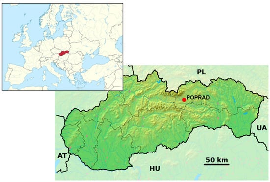
Figure 1.
Location of Poprad in Slovak republic.
2.2. Input Data
For statistical analysis of daily rainfall in the Poprad station, two temporal datasets were used. The first consists of manually recorded daily rainfall data from 1951 to 2018. These data are from an ombrometer, where it was manually recorded every day at 7 a.m. for a period of 67 y. The time series of the recorded daily rainfall data from 1951 to 2018 are shown in Figure 2. The second set of data is daily data, which was derived from automatically recorded 10 min data for the period 2000–2018. Time series of recorded daily rainfall data derived from 10 min of data for the period 2000–2018 is shown in Figure 3. These two types of data were used because of their different ways of obtaining, both of which refer to daily precipitation totals. The main goal of the study is a statistical analysis of daily precipitation totals, but a partial result is the comparison of these two types of data. All these data were provided by Slovak hydrometeorological institute (SHMI), and it is necessary to note that for both time series there were no missing data. The differences between these two datasets are the data collection method (manually vs. automatically) and observation length (67 vs. 18 y). The complex analysis includes basic statistics, trend, stationarity, homogeneity, periodicity and noise for the short-term time series.
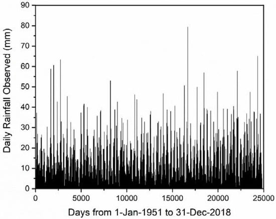
Figure 2.
Daily rainfall time series (recorded): 67 y.
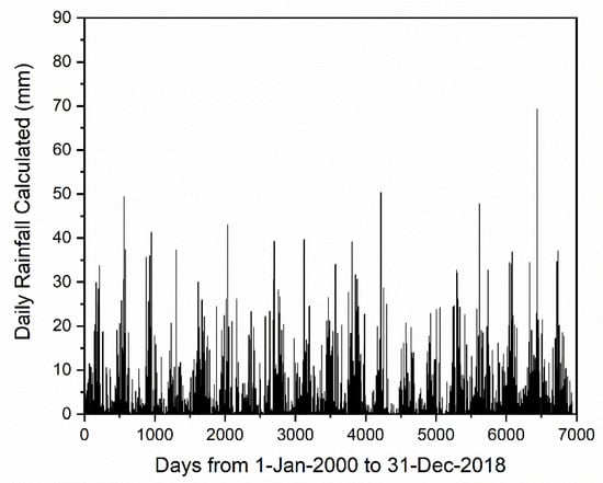
Figure 3.
Daily rainfall time series: developed (calculated) from 10 min to 18 y.
2.3. Descriptive and Statistical Analysis
The first task was the comparison of both rainfall time series. Even though the process is the same due to the different ways of data collection there may be some errors in the magnitude; these errors need to be first checked in the time series. The comparison of these time series is shown in Figure 4, and differences are described in the following sections. The data were compared only for the common time period that is from 1 January 2000 to 31 December 2018.
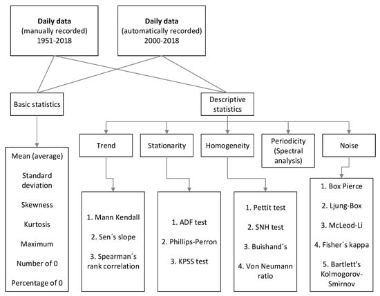
Figure 4.
Flow chart of methodology used in the study (modified according to Drissia et al., 2018 [2]).
As is visible from Figure 4, we can see a strong dependency between data in the scatter plot, except for a few days, which is proved also by the Pearson correlation coefficient in the next section. From 10 min of data, the daily data were calculated. Because the manually recorded data are showing the rainfall amount for one day from the time period from 7 a.m. to 7 a.m. the next day, the same we did with the 10 min of data. Daily data were compared by graphic visualization and by using the Pearson correlation coefficient.
Secondly, the temporal variation in the rainfall data time series was analyzed using a series of statistical tests of trend, stationarity, homogeneity, periodicity and noise. The methodology and types of tests used to analyze the temporal variation of Poprad rainfall in the present study are shown in Figure 4.
As shown in Figure 4, the statistical analysis was divided into basic statistics and descriptive statistics. Basic statistics consist of the mean (average), standard deviation, skewness, kurtosis, maximum, number of zeroes and percentage of zeroes, which presents the number of days without rainfall. Descriptive statistics consist of trend analysis, stationarity, homogeneity, periodicity and noise tests. The trend in the time series is estimated using the Mann–Kendall (MK) test [24], Sen’s slope [25] and Spearman’s rank correlation [26]. The results of the trend analysis show the general trend in time series, but for the behavior of the mean and variance in time there are stationarity tests. The stationarity of time series was tested by the ADF test [27], Phillips–Perron test [28] and KPSS test [29]. Homogeneity tests also indicate the variations in the time series and also give the breakpoint where changes happened in time series. Homogeneity tests used in the present study are the Pettit test [30], SNH test [31], Buishand’s test [32], Von Neumann ratio [33]. For determining white noise in time series, Box–Pierce [34], Ljung–Box [35], McLeod–Li [36], Fisher’s kappa [37] and Bartlett’s Kolmogorov–Smirnov [38] tests are used. For determining the periodicity of time series, spectral analysis was used. The periodic behavior of a time series is observed by utilizing the sine wave function of a time series. The periodicity that gives the strength of the time series at a given frequency is presented by periodogram. The peak value of the periodogram is the dominant frequency [39]. All the tests were carried out at a 5% significance level. In all the tests, p-value is calculated, and if the p-value is less than 0.05 (5% significance level), then the null hypothesis is rejected, and the alternative hypothesis is accepted.
3. Results and Discussion
The first task was the comparison of both rainfall time series. Even though the process is the same due to the different ways of data collection there may be some errors in the magnitude, these errors need to be first checked in the time series. The comparison of these time series is shown in Figure 5 and differences are described in the following sections. The data were compared only for the common time period that is from 1 January 2000 to 31 December 2018.
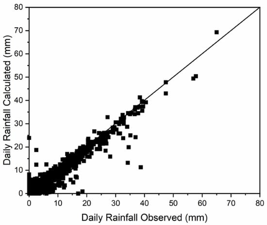
Figure 5.
Relation between time series.
As it is visible from Figure 5, we can see a strong dependency between data in the scatter plot, except for a few days, which is proved also by the Pearson correlation coefficient in the next section. From 10 min of data, the daily data were calculated. Because the manually recorded data are showing the rainfall amount for one day from the time period from 7 a.m. to 7 a.m. the next day, the same we did with the 10 min of data. Daily data were compared by graphic visualization and by using the Pearson correlation coefficient.
Only a small difference between automatically and manually recorded data is expected, which may sometimes lead to erroneous behavior in the long-term that may be also inferred as noise in the data. Both time series look very similar with small deviations and the Pearson correlation coefficient is 0.973. It means that there is a strong correlation between these two time series. The analysis of all the three rainfall series is shown in Table 1.

Table 1.
Differences between time series.
The time series of rainfall at Poprad station are similar in characteristics, which is obvious from the correlation of both time series and also from graphic visualization of time series. There are only small differences (total of rainfall, or maximum rainfall), but it is based on different manners in the collection of the data. For further analysis, manually recorded rainfall data time series was chosen. It is because of the length of the time series.
3.1. Basic Statistical Analysis
The statistical analysis (basic statistics and descriptive statistics) were first carried out for manually recorded daily rainfall data from 1.1.1951 to 31.12.2018 in Poprad, and then for calculated rainfall series. The results of these analyses are described below. The average daily rainfall in Poprad from 1951 to 2018 is 1.6 mm/d, the maximum daily rainfall was 79.3 mm/d on 28.8.1996. The highest daily rainfall in Poprad is during the summer season in June, July and August (average 2.689 mm/d). On the other hand, the lowest rainfall is in the winter season, especially from January to March (average 0.89 mm/d). Time distribution of daily rainfall during the year is shown in Figure 6 where is presented annual average (mean) and standard deviation of daily rainfall in Poprad station for the evaluated period (1951–2018).
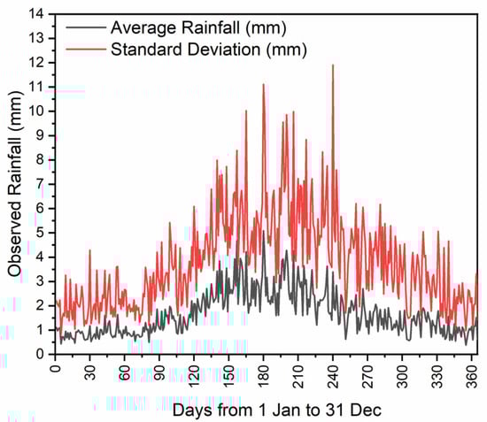
Figure 6.
Annual average and standard deviation of daily rainfall.
In the next figures, the properties (such as average, standard deviation, number of days without rainfall presented by number and percentage of days without rainfall, or maximum rainfall) of time series are shown. In Figure 7, average daily rainfall (mean) and standard deviation of daily rainfall in Poprad station for the last 68 years (1951 to 2018) is reported.
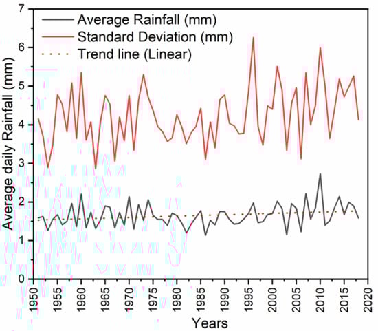
Figure 7.
Mean and standard deviation of daily rainfall from 1951 to 2018.
The figure shows that there is slight increasing trend in the average daily rainfall over the past 68 years. The highest average daily rainfall was in 2010 and it was 2.73 mm/d. On the other hand, the lowest average daily rainfall was in 1986 and it was 1.13 mm/d, which is less than half of the maximum in 2010. Average daily rainfall for the entire observation period is 1.8 mm/d. These results show that the average daily rainfall for the last 68 years is constant, without any major changes and still oscillates around 1.8 mm/d.
The occurrence of dry days during one year for the observed period is shown in Figure 8 and is expressed by number and percentage of days without rainfall for the same day in the year for the range of the years 1951–2018.
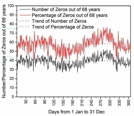
Figure 8.
Average number and percentage of days without rainfall during the year.
The results show that the minimum dry days occur in May and June, while the highest number of days without rainfall occur in August and September. The Figure 8 shows the time distribution of days without rainfall over the one year.
The average number of days without rainfall (dry days) and rainy days for each year from 1951 to 2018 are visible in Figure 9. The trend of rainy and non-rainy days is also plotted in Figure 9. It is clear that the number of dry days per year varies significantly from 180 to 240 d. The chart shows that the number of days without rain that occurs in the year is increasing. In conjunction with the increase in the total annual rainfall and the constant average daily rainfall, this means an increase in extreme precipitation events, as a larger annual rainfall is divided into fewer rainy days, while all are more intense. This conclusion is also shown in Figure 10, which shows the increasing trend of maximum daily precipitation for each year over the reporting period.
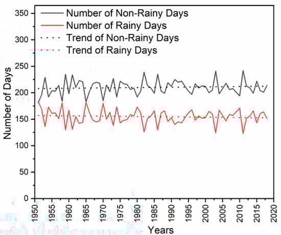
Figure 9.
Number of days without rainfall for each year from 1951 to 2018.
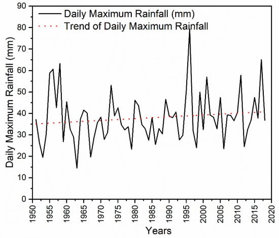
Figure 10.
Maximum of daily rainfall for each year from 1951 to 2018.
It is further confirmed through annual rainfall shown in Figure 11. Overall, the average daily rainfall is showing a significant increasing trend, with a decreasing trend in the number of rainy days and a significant increasing trend in annual rainfall. However, this pictorial analysis has to be confirmed with a statistical method of trend analysis and is discussed in the following section.
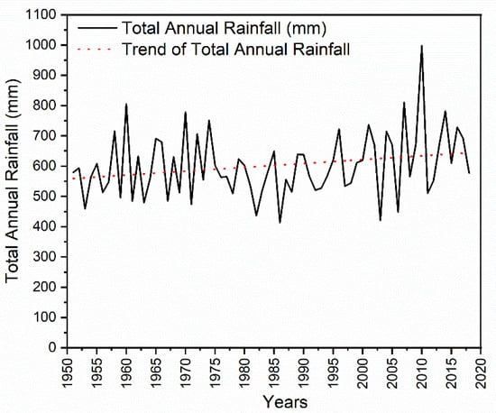
Figure 11.
Total annual rainfall for each year from 1951 to 2018.
3.2. Descriptive Statistical Analysis
Descriptive statistical analysis consists of trend, stationarity, homogeneity, periodicity and noise tests and was done on time series of daily rainfall. A description of each method is given in the Material and Methods section. The results of descriptive statistical analysis are listed in Table 2.
Table 2.
The results of descriptive analysis.
3.2.1. Trend Analysis of Daily Rainfall
The trend in the daily rainfall time series was estimated using the MK test, Sen’s slope test and Spearman’s rank correlation coefficient methods. Globally we can say that there is no trend in the time series. Mann–Kendall test can be interpreted by two hypotheses: H0—There is no trend in the series and Ha—There is a trend in the series. As the computed p-value (0.598) is greater than the significance level alpha = 0.05, the null hypothesis H0 cannot be rejected. Calculated Sen’s slope is 0.00, which means that there is no slope (inclination) of the trend line. Spearman’s rank correlation coefficient is 0.34, which means weak negligible trend in time series.
3.2.2. Stationarity, Homogeneity, Noise and Periodicity of Daily Rainfall
The stationarity test was carried out by the ADF test and Phillips–Perron test where hypothesis H0 is that there is a unit root for the series and hypothesis Ha is that there is no unit rood for the series and the series is stationary. Another test for stationarity is the KPSS test, where hypothesis H0 is that the series is stationary and hypothesis Ha is that the series is not stationary. The result of all the three methods concludes that the daily rainfall series in Poprad station is significantly stationary at a 5% significance level as shown in Table 2. It means that any hydrologic model can be used for modeling daily rainfall. It can be concluded that the daily rainfall series is not showing much variation in mean and standard deviation, which is also evident from Figure 7.
The homogeneity was tested using Pettitt’s test, standard normal homogeneity (SNH) test, Buishand test and von Neumann’s test. In all tests for homogeneity, the hypothesis H0 is that data are homogeneous and hypothesis Ha is that there is a date at which there is a change in the data what means that time series is not homogeneous. The time series of daily rainfall in Poprad station is homogeneous, which was proven by all four tests at a 5% significance level. It means that there is no breakpoint in the time series.
The presence of white nose in the daily rainfall time series was tested using Box–Pierce, Lying-Box and McLeod–Li tests. White noise is in time series when the p-value is larger than the significance level alpha. All the tests confirmed that there is no noise in the daily rainfall time series in Poprad station. The p-value was found to be 0.0001, which is less than alpha = 0.05 using all four methods.
The periodicity test is used to identify the behavior of a time series [40]. The periodogram was plotted for the time series. In daily rainfall time series, the period is 365.25 d, which means that it takes 365.25 d to complete one cycle. The periodicity is not exactly 365.00 because of leap year, which happens once in four years.
4. Conclusions
The analysis of the precipitation concentration degree throughout the year is extremely important for its high impact on environmental phenomena like floods and droughts. For the observed Poprad station, two types of analysis were conducted. The basic statistical analyses showed results which give quite a precise picture of the rainfall occurrence during the year and the examined period between the years 1951 and 2018. The average daily rainfall in Poprad during the mentioned period is 1.6 mm/d, the maximum daily rainfall was 79.3mm/d on 28.8.1996. The highest daily rainfall in Poprad is during the summer season in June, July and August (average 2.689 mm/d). On the other hand, the lowest rainfall is in the winter season, especially from January to March (average 0.89 mm/d). Most of the dry days during the year occur in August and September. The data also show that the number of dry days is increasing, but in conjunction with the increase in the total annual rainfall and the constant average daily rainfall, this means an increase in extreme precipitation events, as a larger annual rainfall is divided into fewer rainy days, while all are more intense. For the observed Poprad station the tests on trend, homogeneity, stationarity, periodicity and noise has been conducted. As a result, all approaches used in this paper are indicating no trend or wear a negligible trend. The tests on stationarity are classifying data set of rainfall as stationary. All four tests on homogeneity are showing that the data are homogenous. An interesting result brought the test on periodicity when the value of periodicity was 365,25 d which means exactly one year and the part of the day from the leap year. The test of noise also showed no noise on data.
Author Contributions
Conceptualization, M.Z. and V.J.; methodology, V.J.; software, A.R.; validation, A.R., M.Z. and V.J.; formal analysis, I.M.; investigation, A.R.; resources, H.H.; data curation, H.H.; writing—original draft preparation, A.R.; writing—review and editing, I.M.; visualization, V.J.; supervision, M.Z.; project administration, V.J.; funding acquisition, M.Z. All authors have read and agreed to the published version of the manuscript.
Funding
This research received no external funding.
Acknowledgments
This work was supported by projects of the Ministry of Education of the Slovak Republic VEGA 1/0217/19 Research of Hybrid Blue and Green Infrastructure as Active Elements of a Sponge City, VEGA 1/0308/20 Mitigation of hydrological hazards, floods and droughts, by exploring extreme hydroclimatic phenomena in river basins, the project od Slovak Research and Development Agency APVV-18-0360 Active hybrid infrastructure towards to sponge city and project HUSKROUA/1702/6.1/0072 Innovative sustainable water management practices for urban areas via integrated watershed water management C.
Conflicts of Interest
The authors declare no conflict of interest.
References
- Chow, V.T.; Maidment, D.R.; Mays, L.W. Applied Hydrology; International edition; McGraw-Hill, Inc.: New York, NY, USA, 1988; p. 350. [Google Scholar]
- Drissia, T.K.; Jothiprakash, V.; Anitha, A.B. Statistical classification of streamflow based on flow variability in west flowing rivers of Kerala, India. Theor. Appl. Climatol. 2019, 137, 1643–1658. [Google Scholar] [CrossRef]
- Praveenkumar, C.; Jothiprakash, V. Spatio-temporal trend and homogeneity analysis of gridded and gauge precipitation in Indravati River basin, India. J. Water Clim. Chang. 2020, 11, 178–199. [Google Scholar] [CrossRef]
- Zeleňáková, M.; Alkhalaf, I.; Purcz, P.; Blišt’an, P.; Pelikán, P.; Portela, M.; Silva, A. Trends of rainfall as a support for integrated water resources management in Syria. Desalin. Water Treat. 2017, 86, 285–296. [Google Scholar] [CrossRef]
- Zeleňáková, M.; Vido, J.; Portela, M.M.; Purcz, P.; Blištán, P.; Hlavatá, H.; Hluštík, P. Precipitation Trends over Slovakia in the Period 1981–2013. Water 2017, 9, 922. [Google Scholar] [CrossRef]
- Zeleňáková, M.; Purcz, P.; Blišt’an, P.; Alkhalaf, I.; Hlavata, H.; Portela, M.M.; Silva, A.T. Precipitation trends detection as a tool for integrated water resources management in Slovakia. Desalin. Water Treat. 2017, 99, 83–90. [Google Scholar] [CrossRef]
- Zeleňáková, M.; Jothiprakash, V.; Arjun, S.; Káposztásová, D.; Hlavatá, H. Dynamic Analysis of Meteorological Parameters in Košice Climatic Station in Slovakia. Water 2018, 10, 702. [Google Scholar] [CrossRef]
- Afzal, M.; Mansell, M.G.; Gagnon, A.S. Trends and variability in daily precipitation in Scotland. Procedia Environ. Sci. 2011, 6, 15–26. [Google Scholar] [CrossRef]
- Gong, D.Y.; Shi, P.J.; Wang, J.A. Daily precipitation changes in the semi-arid region over northern China. J. Arid Environ. 2004, 59, 771–784. [Google Scholar] [CrossRef]
- Croitoru, A.E.; Piticar, A.; Burada, D.C. Changes in precipitation extremes in Romania. Quat. Int. 2016, 415, 325–335. [Google Scholar] [CrossRef]
- Keggenhoff, I.; Elizbarashvili, M.; Amiri-Farahani, A.; King, L. Trends in daily temperature and precipitation extremes over Georgia, 1971–2010. Weather Clim. Extrem. 2014, 4, 75–85. [Google Scholar] [CrossRef]
- Caloiero, T.; Coscarelli, R.; Ferrari, E.; Sirangelo, B. Trends in the daily precipitation categories of Calabria (southern Italy). Procedia Eng. 2016, 162, 32–38. [Google Scholar] [CrossRef]
- Zubieta, R.; Saavedra, M.; Silva, Y.; Giráldez, L. Spatial analysis and temporal trends of daily precipitation concentration in the Mantaro River basin: Central Andes of Peru. Stoch. Environ. Res. Risk Assess. 2017, 31, 1305–1318. [Google Scholar] [CrossRef]
- Bičárová, S.; Holko, L. Changes of characteristics of daily precipitation and runoff in the High Tatra Mountains, Slovakia over the last fifty years. Contrib. Geophys. Geod. 2013, 43, 157–177. [Google Scholar] [CrossRef]
- Gaál, L.; Kyselý, J.; Szolgay, J. Region-of-influence approach to a frequency analysis of heavy precipitation in Slovakia. Hydrol. Earth Syst. Sci. Discuss. 2008, 12, 825–839. [Google Scholar] [CrossRef]
- Bara, M.; Kohnova, S.; Gaal, L.; Szolgay, J.; Hlavčova, K. Estimation of IDF curves of extreme rainfall by simple scaling in Slovakia. Contrib. Geophys. Geod. 2009, 39, 187–206. [Google Scholar]
- Šamaj, F.; Valovič, Š. Intenzity Krátkodobých Dažďov na Slovensku; Slov. Pedagog. Nakl.: Bratislava, Slovakia, 1973; p. 93. [Google Scholar]
- Dub, O.; Nemec, J. Hydrologie; Státní Nakladatelství Technické Literatury: Praha, Czech Republic, 1969; p. 378. [Google Scholar]
- Kottegoda, N.T. Stochastic Water Resources Technology, 1st ed.; The Macmillan Press Ltd.: London, UK, 1980; p. 384. [Google Scholar]
- Chatfield, C. Time Series Forecasting; Chapman & Hall/CRC: London, UK, 2000. [Google Scholar]
- Dahmen, E.R.; Hall, M.J. Screening of Hydrological Data: Tests for Stationarity and Relative Consistency; International Institute for Land Reclamation and Improvement: Wageningen, The Netherlands, 1990. [Google Scholar]
- Akinsanola, A.A.; Ogunjobi, K.O. Recent homogeneity analysis and long-term spatio-temporal rainfall trends in Nigeria. Theor. Appl. Clim. 2015, 128, 275–289. [Google Scholar] [CrossRef]
- Anděl, J. Statistická Analýza Časových Řad; Státní Nakladatelství Technické Literatury: Praha, Czech Republic, 1976; p. 272. [Google Scholar]
- Gilbert, R.O. Statistical Methods for Environmental Pollution Monitoring; John Wiley & Sons: Hoboken, NJ, USA, 1987. [Google Scholar]
- Sen, P.K. Estimates of the regression coefficient based on Kendall’s tau. J. Am. Stat. Assoc. 1968, 63, 1379–1389. [Google Scholar] [CrossRef]
- Gautheir, T.D. Detecting trends using Spearman’s rank correlation coefficient. Environ. Forensics 2001, 2, 359–362. [Google Scholar] [CrossRef]
- Dickey, D.A.; Fuller, W.A. Distribution of the estimators for autoregressive time series with a unit root. J. Am. Stat. Assoc. 1979, 74, 427–431. [Google Scholar]
- Phillips, P.C.; Perron, P. Testing for a unit root in time series regression. Biometrika 1988, 75, 335–346. [Google Scholar] [CrossRef]
- Kwiatkowski, D.; Phillips, P.C.; Schmidt, P.; Shin, Y. Testing the null hypothesis of stationarity against the alternative of a unit root. J. Econ. 1992, 54, 159–178. [Google Scholar] [CrossRef]
- Pettitt, A.N. A non-parametric approach to the change-point problem. J. R. Stat. Soc. Ser. C (Appl. Stat.) 1979, 28, 126–135. [Google Scholar] [CrossRef]
- Alexandersson, H.; Moberg, A. Homogenization of Swedish temperature data. Part I: Homogeneity test for linear trends. Int. J. Climatol. J. R. Meteorol. Soc. 1997, 17, 25–34. [Google Scholar]
- Buishand, T.A.; De Haan, L.; Zhou, C. On spatial extremes: With application to a rainfall problem. Ann. Appl. Stat. 2008, 2, 624–642. [Google Scholar] [CrossRef]
- Von Neumann, J. Distribution of the ratio of the mean square successive difference to the variance. Ann. Math. Stat. 1941, 12, 367–395. [Google Scholar] [CrossRef]
- Box, G.E.; Pierce, D.A. Distribution of residual autocorrelations in autoregressive-integrated moving average time series models. J. Am. Stat. Assoc. 1970, 65, 1509–1526. [Google Scholar] [CrossRef]
- Ljung, G.M.; Box, G.E. On a measure of lack of fit in time series models. Biometrika 1978, 65, 297–303. [Google Scholar] [CrossRef]
- McLeod, A.I.; Li, W.K. Diagnostic checking ARMA time series models using squared-residual autocorrelations. J. Time Ser. Anal. 1983, 4, 269–273. [Google Scholar] [CrossRef]
- Fisher, R.A. Statistical methods for research workers. In Breakthroughs in Statistics; Springer: New York, NY, USA, 1992; pp. 66–70. [Google Scholar]
- Bartlett, M.S. An Introduction to Stochastic Processes: With Special Reference to Methods and Applications; CUP Archive: London, UK, 1978. [Google Scholar]
- Schuster, A. On the investigation of hidden periodicities with application to a supposed 26 day period of meteorological phenomena. Terr. Magn. 1989, 3, 13–41. [Google Scholar] [CrossRef]
- Elfeky, M.G.; Aref, W.G.; Elmagarmid, A.K. Periodicity detection in time series databases. IEEE Trans. Knowl. Data Eng. 2005, 17, 875–887. [Google Scholar] [CrossRef]
© 2020 by the authors. Licensee MDPI, Basel, Switzerland. This article is an open access article distributed under the terms and conditions of the Creative Commons Attribution (CC BY) license (http://creativecommons.org/licenses/by/4.0/).