Article

Projecting Wet Season Rainfall Extremes Using Regional Climate Models Ensemble and the Advanced Delta Change Model: Impact on the Streamflow Peaks in Mkurumudzi Catchment, Kenya

by
Wendso Awa Agathe Ouédraogo
1,*,
John Mwangi Gathenya
2 and
James Messo Raude
2
1
Civil Engineering Department, Pan African University – Institute for Basic Sciences Technology and Innovation/Jomo Kenyatta University of Agriculture and Technology, P.O. Box 62000-00200 Nairobi, Kenya
2
Soil, Water & Environmental Engineering Department/Jomo Kenyatta University of Agriculture and Technology, P.O. Box 62000-00200 Nairobi, Kenya
*
Author to whom correspondence should be addressed.
Hydrology 2019, 6(3), 76; https://doi.org/10.3390/hydrology6030076
Submission received: 19 July 2019 / Revised: 18 August 2019 / Accepted: 23 August 2019 / Published: 26 August 2019

Abstract

:
Each year, many African countries experience natural hazards such as floods and, because of their low adaptative capabilities, they hardly have the means to face the consequences, and therefore suffer huge economic losses. Extreme rainfall plays a key role in the occurrence of these hazards. Therefore, climate projection studies should focus more on extremes in order to provide a wider range of future scenarios of extremes which can aid policy decision making in African societies. Some researchers have attempted to analyze climate extremes through indices reflecting extremes in climate variables such as rainfall. However, it is difficult to assess impacts on streamflow based on these indices alone, as most hydrological models require daily data as inputs. Others have analyzed climate projections through general circulation models (GCMs) but have found their resolution too coarse for regional studies. Dynamic downscaling using regional climate models (RCMs) seem to address the limitation of GCMs, although RCMs might still lack accuracy due to the fact that they also contain biases that need to be eliminated. Given these limitations, the current study combined both dynamic and statistical downscaling methods to correct biases and improve the reproduction of high extremes by the models. This study’s aim was to analyze extreme high flows under the projection of extreme wet rainfall for the horizon of 2041 of a Kenyan South Coast catchment. The advanced delta change (ADC) method was applied on observed data (1982–2005), control (1982–2005) and near future (2018–2041) from an ensemble mean of multiple regional climate models (RCMs). The created future daily rainfall time series was introduced in the HEC-HMS (Hydrologic Engineering Center’s Hydrologic Modeling System) hydrological model and the generated future flow were compared to the baseline flow at the gaging station 3KD06, where the observed flow was available. The findings suggested that in the study area, the RCMs, bias corrected by the ADC method, projected an increase in rainfall wet extremes in the first rainy season of the year MAMJ (March–April–May–June) and a decrease in the second rainy season OND (October–November–December). The changes in rainfall extremes, induced a similar change pattern in streamflow extremes at the gaging station 3KD06, meaning that an increase/decrease in rainfall extremes generated an increase/decrease in the streamflow extremes. Due to lack of long-term good quality data, the researchers decided to perform a frequency analysis for up to a 50 year return period in order to assess the changes induced by the ADC method. After getting a longer data series, further analysis could be done to forecast the maximum flow to up to 1000 years, which could serve as design flow for different infrastructure.

1. Introduction

The world is experiencing the effects of climate change, with extreme climate events increasing with time, making the situation grow from bad to worse. Developing countries such as those in Africa are more vulnerable due to poverty and low adaptive capacity [1]. Some studies have attempted to investigate rainfall extremes’ variability in recent decades and the future in Africa. Mason et al. [2] investigated changes in extreme rainfall events in South Africa in the 20th century. The authors reported that the intensity of extreme rainfall events has significantly increased in more than half of the country. Fotso-nguermo et al. [3] studied projected rainfall extremes over Central Africa (CA) based on outputs from twenty global climate models (GCMs) of the Coupled Model Intercomparison Project Phase 5 (CMIP5) produced under the RCP8.5 scenario. The authors concluded that extreme rainfall events might become more frequent, thereby worsening flood conditions in CA countries. Ongoma et al. [4] studied the variability of extreme rainfall events over East Africa (EA), using indices from the World Meteorological Organization (WMO) Expert Team on Climate Change Detection and Indices (ETCCDI). Their results showed that the standardized rainfall anomaly increased, especially above normal, which may imply an increase in extreme rainfall events. The annual total precipitation in wet days (PRCPTOT), showed a decrease until the 2000s followed by an increase in the next decade. Gebrechorkos et al. [5] tested the variability of precipitation extremes in the Eastern Africa (Ethiopia, Kenya, and Tanzania) region during 1981–2016. They found significant increasing trends in Kenya for the simple daily intensity index (SDII), the very wet days’ precipitation (R95P), and the extremely wet days’ precipitation (R99P). According to the fifth Intergovernmental Panel on Climate Change (IPCC) report [6], “droughts and storms have been more frequent in Eastern Africa in the last 30–60 years” and IPCC projections expect such events to be more frequent and intense in the near future.
Therefore, there is an urgent need for African countries to anticipate the impacts of extreme events through projection scenarios. Projections have been made using GCMs which were found to have coarse resolution and give only fairly accurate results [7]. Moreover, the GCMs’ outputs involve some biases which can lead to significant errors in impacts studies. One way to improve the accuracy of GCMs is through dynamical downscaling using regional climate models (RCMs). High resolution regional climate models give a better local capturing of important details like mountains, coasts, lakes and vegetation [8,9,10]. They might still lack accuracy when the resolution is not high enough to allow for impacts assessments at a point scale. In addition, outputs from RCMs also contain biases inherited from driving GCMs which need to be eliminated [11]. It was found that a combination of dynamical and statistical downscaling could address the non-accurate projections of the models [12,13,14,15].
Several statistical downscaling methods (also called bias correction methods) have been tested in the past decades [10,11,12], such as the delta change method [16], the multiplicative correction [17], the monthly non-linear correction [18] and the power transformation [19]. Some of the methods consist of correcting the mean error, while others focus on both average and variance or on the correction of mean and standard deviation [20]. A focus on extremes is needed for extreme events analysis. In this study, a more advanced delta method was applied; this approach has the advantage of taking into account both changes in the mean and in the extremes. In addition, a non-linear transformation was applied, rather than a proportional adjustment of observed precipitation.
In recent years, the assessment of hydrological impacts of climate change has been of great interest. The physically-based HEC-HMS (Hydrologic Engineering Center’s Hydrologic Modeling System) model [21] has been used in different parts of the world and was pointed out as an highly adaptable model that includes a variety of model choices for each part of the hydrologic cycle. Rehana et al. [22] used the HEC-HMS model to evaluate the impacts of possible future climate change scenarios on the hydrology of the Tunga–Bhadra River basin in India. They provided, as input, some large-scale climate variables for the A2 and B2 emission scenarios obtained from the Hadley Centre Coupled Model version 3. Tefera [23] assessed the availability of surface water resources in the Beles River basin (Ethiopia), using a surface water balance model simulation by HEC-HMS. Muli N. [24] used the HEC-HMS model to study flood in a Nairobi watershed based on a rainfall-runoff process while considering urban development and its effects on the watershed. Bitew et al. [25] also used the HEC-HMS model to simulate the surface runoff for the Gilgel Abay catchment in Ethiopia. The Soil Conservation Service curve number (SCS-CN), the Soil Conservation Service unit hydrograph (SCS-UH) and the Muskingum methods were applied for loss, runoff estimation, and flow routing, respectively. Ouédraogo et al. [26], the authors of the current study, performed a calibration, validation, performance evaluation and sensitivity analysis for the HEC-HMS model in the Mkurumudzi catchment. The Soil Moisture Accounting (SMA) loss method, combined with the canopy and surface methods, was applied to model the infiltration losses. The Soil Conservation Service unit hydrograph (SCS-UH) and the Lag methods were applied for the runoff estimation and flow routing, respectively. Based on the performance results, the model was found suitable to model streamflow in the Mkurumudzi catchment.
The objective of the current study was to analyze extreme high flows under the projection of the extreme rainfall for horizon 2041. This objective was met through: (1) The assessment of the accuracy of the Climate Hazards Group InfraRed Precipitation with Station (CHIRPS) data in comparison with ground-station data, (2) the projection of future rainfall extremes using a combination of dynamic and statistical downscaling method after a performance evaluation and selection of climate models, and (3) a streamflow simulation and frequency analysis under the created projections.

2. Materials and Methods
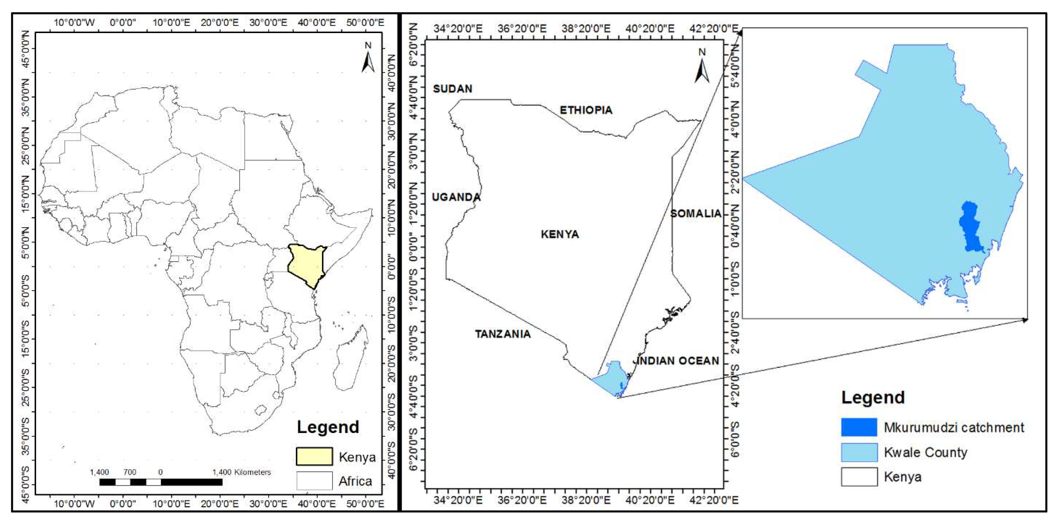
2.1. Study Area

Kenya is a country in East Africa with a coastline on the Indian Ocean (Figure 1) which has 47 smaller administrative units commonly referred to as counties. One such County is Kwale, located in the coast region of Kenya and which covers an approximate area of 8332.2 km2, with an area of 62 km2 uninhabited because it is under water. The county lies between latitude 3°3′ and 4°45′ South and longitude 38°31′ and 39°31′ East, as presented in Figure 1.
Kwale County experiences a monsoon climate with a bimodal rainfall pattern. The long rains fall between March and June (MAMJ), and the short rains fall between October and December (OND). The county receives rainfall in the ranges between 800 and 1600 mm along the coast and 400–600 mm in the hinterland. The temperature ranges from 26.3 to 26.6°C in the coastal lowlands, 25–26.6 °C in the coastal ranges, and 24.6–27.5°C in the hinterlands [27]. The highest mean temperatures are experienced in the months of April and November, while the coolest period is between June and August. The vegetation of the area consists of natural grassland, forested land and typical coastal vegetation palm trees, mango trees, etc., while other areas are cleared and covered with sugarcane plantations. This study focused on the Mkurumudzi catchment, covering an area of 186 km2 (Figure 1).

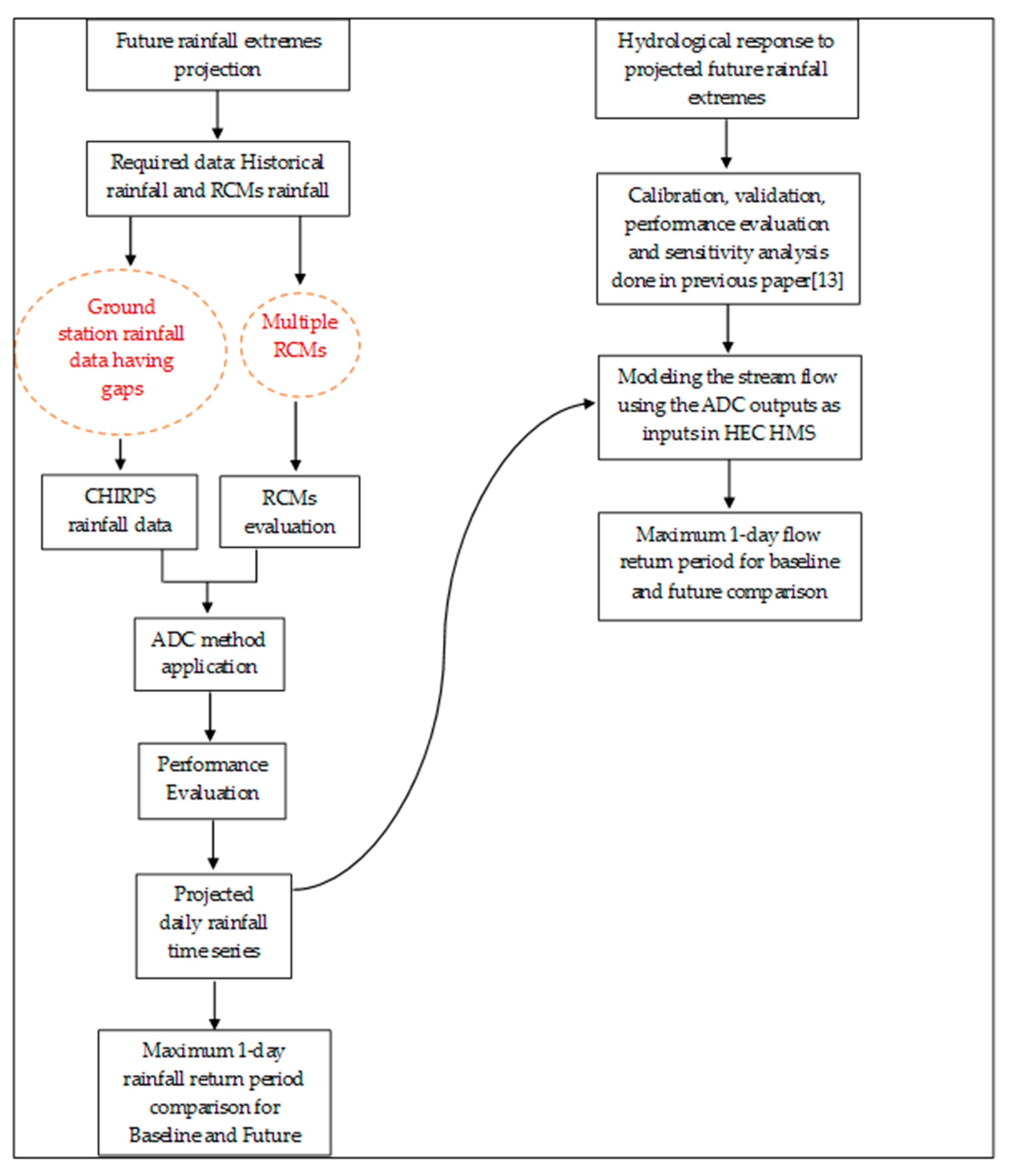
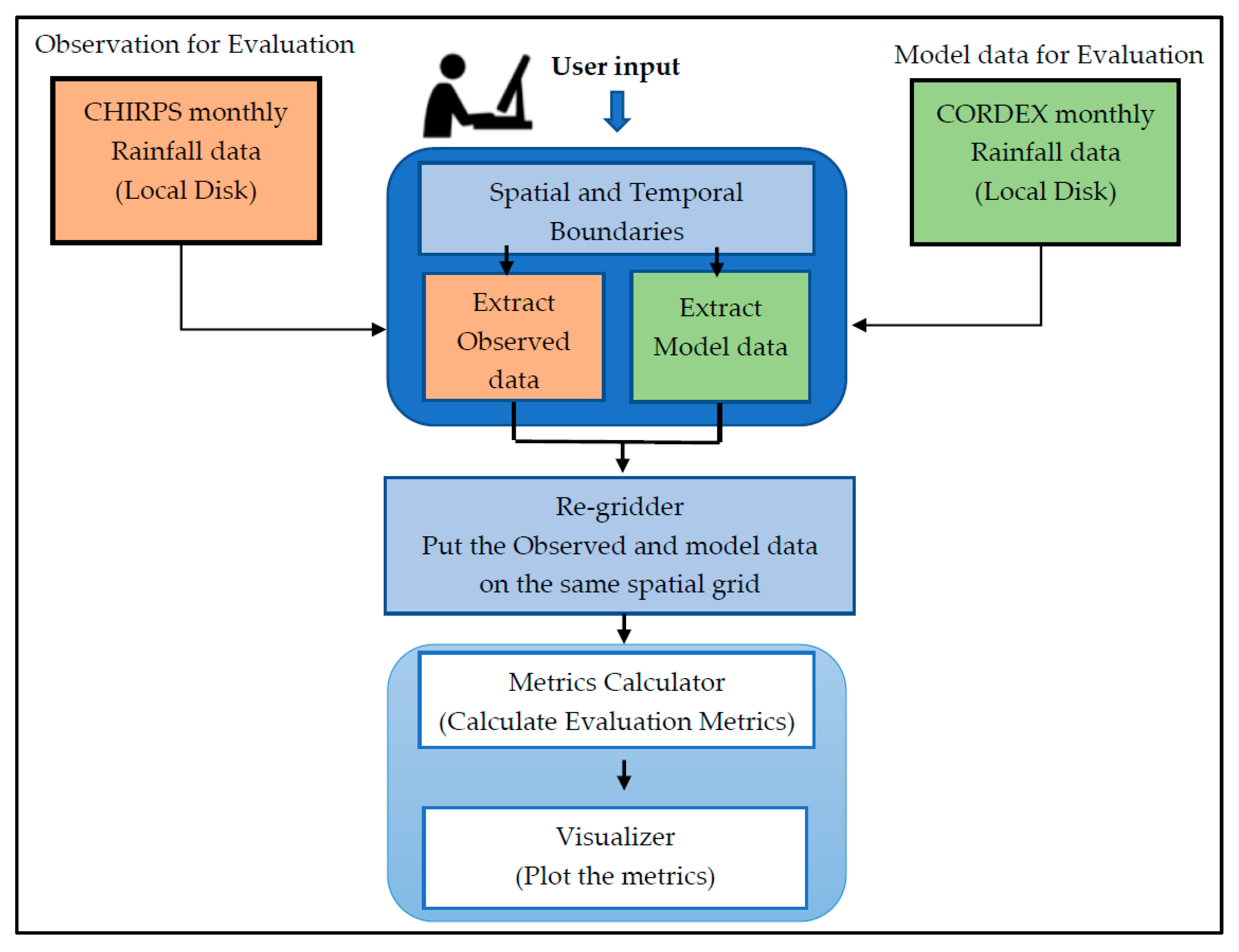
2.2. Flowchart of the Study

The steps taken in this study are highlighted in Figure 2. The methodology consisted of projecting future rainfall extremes and evaluating the hydrological response of the studied catchment to these projections. The advanced delta change (ADC) method was used for the projection and required historical and RCMs’ rainfall data. To address the non-accuracy of the observed ground stations data (due to the presence of gaps), CHIRPS data were evaluated and used instead. A performance evaluation of the RCMs was also conducted to choose the candidate models for the application of the ADC method. The ADC model was validated, and the best performing RCMs were selected and used for further analysis. After the application of the ADC method, the created rainfall time series were put into the HEC-HMS model for the hydrological modeling of the catchment.

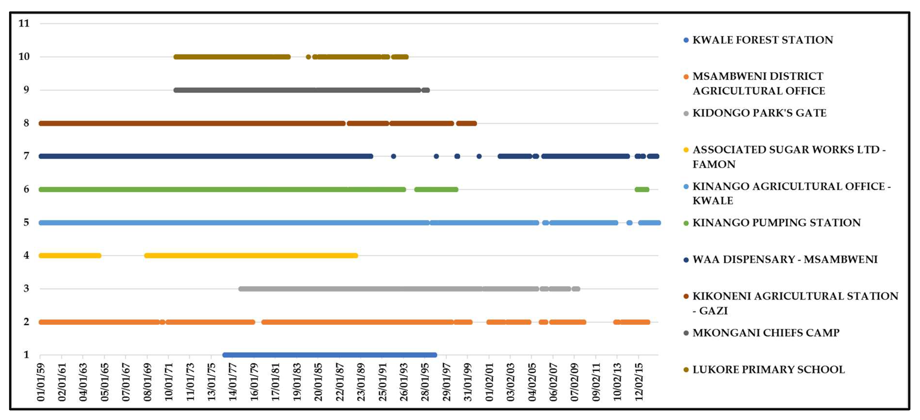
2.3. Available Rainfall Datasets

The current study on extreme rainfall, as is the case with all climate-related studies, required good quality daily observed data [28]. The observed data measured from the ground stations were the best options but, in most cases, especially in Africa, such data sets are difficult to obtain. This is because it is difficult to install and maintain a network of rainfall stations with the capability of providing rainfall data in real time. Even if the data are available, they have some gaps. For instance, Figure 3 shows the rainfall data availability graph from stations in the study area. The data used to create the graphs are from a network of ten ground stations within the study area for a 47-year period (1959–2016). The full horizontal lines represent the available data, while the breaks represent the periods with missing data. The data were obtained from the Kenya Meteorological Department (KMD), the government agency entrusted with the collection and storage of meteorological data. Therefore, satellite precipitation estimates are a very attractive option, because they provide continuous spatial estimates of precipitation.
The Climate Hazards Group InfraRed Precipitation with Station data (CHIRPS) is a 30+ year quasi-global rainfall dataset, spanning from 50 °S to 50 °N (and all longitudes), starting in 1981 to near-present. The CHIRPS incorporates a 0.05° resolution satellite imagery with in-situ station data to create gridded rainfall time series for trend analysis and seasonal drought monitoring [28]. Data can be extracted for points using geographic coordinates. Some efforts have gone into evaluating the accuracy of the Climate Hazards Group products [29]. The authors found CHIRPS rainfall product suitable as an alternative source of rainfall information for their study areas. This study used the same principle to evaluate the accuracy of CHIRPS data within the Mkurumudzi catchment.

2.4. Evaluation Metrics

For the purpose of performance evaluation, both KMD and CHIRPS rainfall data were compared to assess their goodness-of-fit on a monthly and an annual time step, respectively. The comparison was done for the period 1981–2016, as CHIRPS data start from 1981 and observed data stop at 2016. Legates and Mccabe [30] and Moriasi et al. [31] recommended that a good model efficiency evaluation criterion should have at least three important components: One dimensionless statistic, one absolute error index statistic and one graphical technique. This means that none of the statistics are used alone, but when applied together, they form a set of model performance evaluation criteria which offsets the limitation of each other. Therefore, in this study, the following statistics in addition to the coefficient of correlation which is limited by its oversensitivity to outliers and its insensitivity to additive and proportional differences between satellite and observed data [30] were used:
(a)
The coefficient of correlation (R2), which describes the percentage of the variance in observed data explained by the satellite. R2 ranges from 0 to 1, where values greater than 0.5 are considered acceptable [32,33].
R 2 = [ i = 1 n ( O i O ¯ ) x ( S i S ¯ ) i = 1 n ( O i O ¯ ) 2 x i = 1 n ( S i S ¯ ) 2 ] 2
where Oi and Si are the observed and satellite rainfall at time I, respectively, and Ō and S ¯ are the average observed and satellite rainfall during the evaluation period, respectively.
(b)
The dimensionless statistic: Index of agreement (d) was used and is given by:
d = 1 1 = 1 n ( O i S i ) 2 i = 1 n ( | S i O ¯ | + | O i O ¯ | ) 2
The index of agreement complements R2 by its ability to detect the additive and relative variations in the observed and simulated averages and variances. According to Willmott [32], d varies between 0 (absolutely no agreement between the observed and the satellite rainfall) and 1 (perfect agreement).
(c)
The absolute error index represented by the RSR (RMSE standard deviation ratio) given by:
RSR = i = 1 n ( O i S i ) 2 i = 1 n ( O i   O ¯ ) 2
The RSR is recommended over the RMSE because it combines both an absolute error index and the supplementary information suggested by [30]. The RSR ranges from 0 (optimal value) to a larger positive value, indicating poor performance. A lower value of RSR indicates a lower root mean squared error, which indicates the rightness of the satellite [31]. The general performance ratings for the statistics are presented in Table 1.

2.5. Projection of Future Rainfall Extremes Using the Advanced Delta Change Approach on Regional Climate Models Output

The classic delta change method [12] describes a linear transformation of mean precipitation values, which may result in an unrealistic change of the precipitation distribution compared to the changes that occur in the GCMs. However, detailed insight in the change of the extremes in the precipitation distribution is valuable for research and modeling, as many environmental processes are triggered only by extreme low or high precipitation amounts, e.g., flooding, erosion and vegetation stress. To accommodate this, a revised version of the delta change method was proposed by [34], who called it the advanced delta change (ADC) method. For the application, the authors used GCMs from the Coupled Model Intercomparison Project Phase 3 (CMIP3). This study used the regional climate models (RCMs) outputs, from the Coordinated Regional climate Downscaling Experiment (CORDEX), driven by GCMs from the Coupled Model Intercomparison Project Phase 5 (CMIP5). The RCMs outputs were produced under the Representative Concentration Pathway (RCP 8.5). Before the application of the ADC method, a performance evaluation of the climate models’ outputs was undertaken in order to use the data that best fits the study area.

2.5.1. CORDEX Africa Rainfall Data

The CORDEX (Coordinated Regional Climate Downscaling Experiment) program is a framework that was initiated by the World Climate Research Program (WCRP) to evaluate regional climate model performance through a set of experiments aimed at producing regional climate projections. Twenty-one RCMs were evaluated in this study (Table 2). These RCMs were considered for the African domain at a resolution of 0.44 × 0.44 degrees from the historical experiment. Because CHIRPS and RCMs data were available for different periods, this study considered only the overlap period between 1981 and 2005 on a monthly time step. The Regional Climate Model Evaluation System (RCMES) is a system that provides an evaluation tool for RCMs using observations. The RCMES system requires three main elements to function: An observations database (which in this study was the CHIRPS data), CORDEX models outputs, and RCMES toolkits. The first step involves loading the observations and models datasets. Once the datasets are loaded, RCMES spatially subsets the datasets, optionally re-grids the subset datasets, compares the re-gridded datasets, calculates model performance metrics, and visualizes/plots the metrics. The processed observational and model datasets are saved in a NetCDF file. All these model evaluation processes are controlled by the user’s input [35]. Detailed information about the software installation and tutorials can be found in [36]. The RCMES workflow can be found in Figure A1 in Appendix B.
The following two criteria defined by [3] were used to select the best models:
-
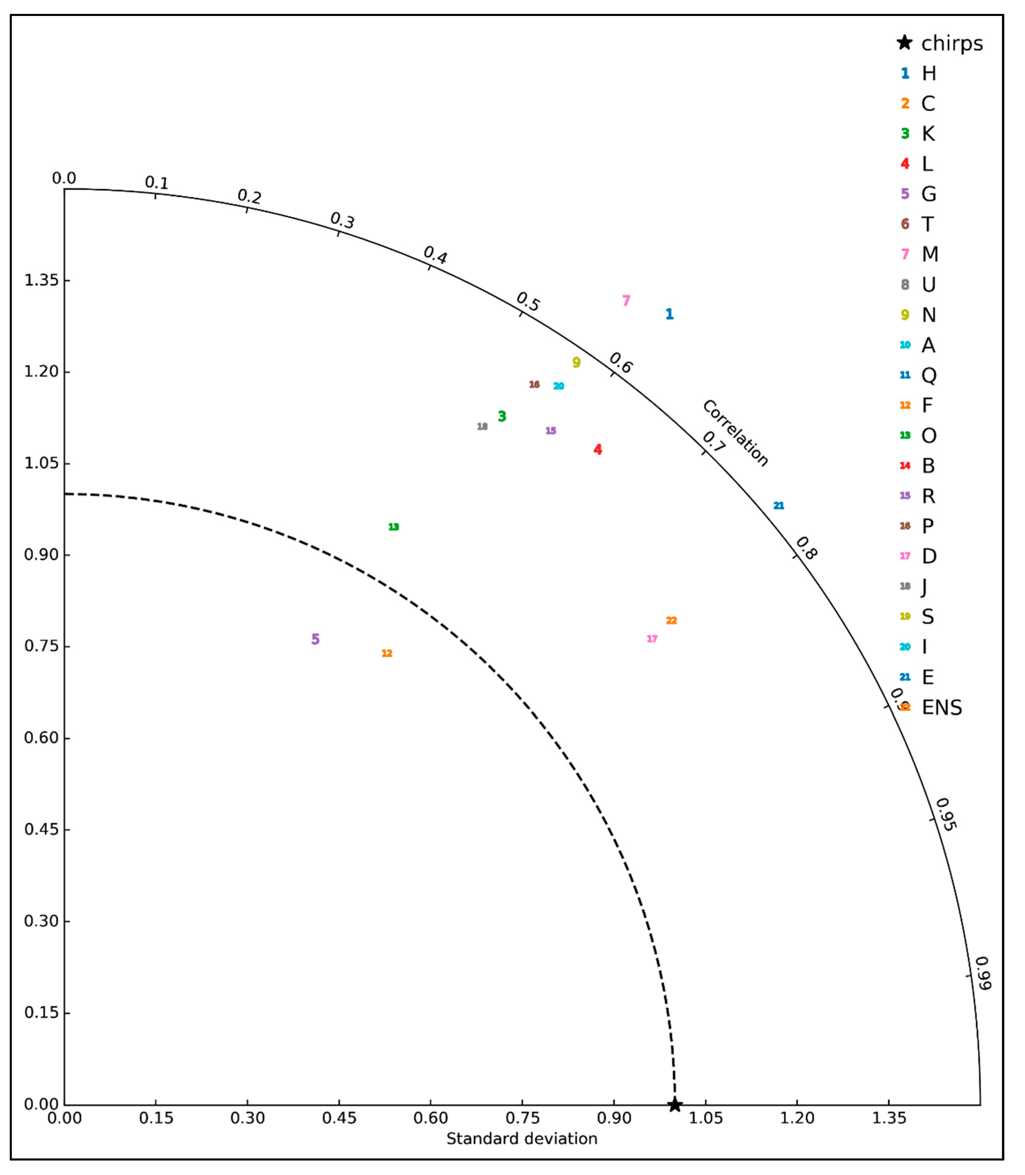
The pattern correlation ≥0.6.
-
the standard deviation ratio within the range of 1.00 ± 0.25.
Many factors have to be taken into consideration when projecting climate change. A key variable is the amount of future greenhouse gas emission. The Intergovernmental Panel on Climate Change (IPCC) in the fifth assessment report (AR5) [6] created a new set of scenarios to provide time-dependent projections of atmospheric greenhouse gas (GHG) concentrations. These scenarios, called Representative Concentration Pathways (RCPs), are characterized by four different types of radiative forcing: One rising pathway for which the radiative forcing reaches >8.5 Watts/m2 by 2100 and continues to rise for some amount of time, RCP8.5 [37]; two intermediate “stabilization pathways” in which the radiative forcing is stabilized at approximately 6 Watts/m2 (RCP6.0) and 4.5 Watts/m2 (RCP4.5) after 2100 [38,39]; and one pathway where radiative forcing peaks at approximately 3 Watts/m2 before 2100 and then declines to 2.6 Watts/m2 by 2100 (RCP2.6) [40]. In this study, the RCP8.5 was chosen, due to the high GHG concentration level and the fact that the study was on extremes under the most pessimistic situation. All available RCMs outputs for Africa and under RCP8.5 were evaluated and are presented in Table 2.

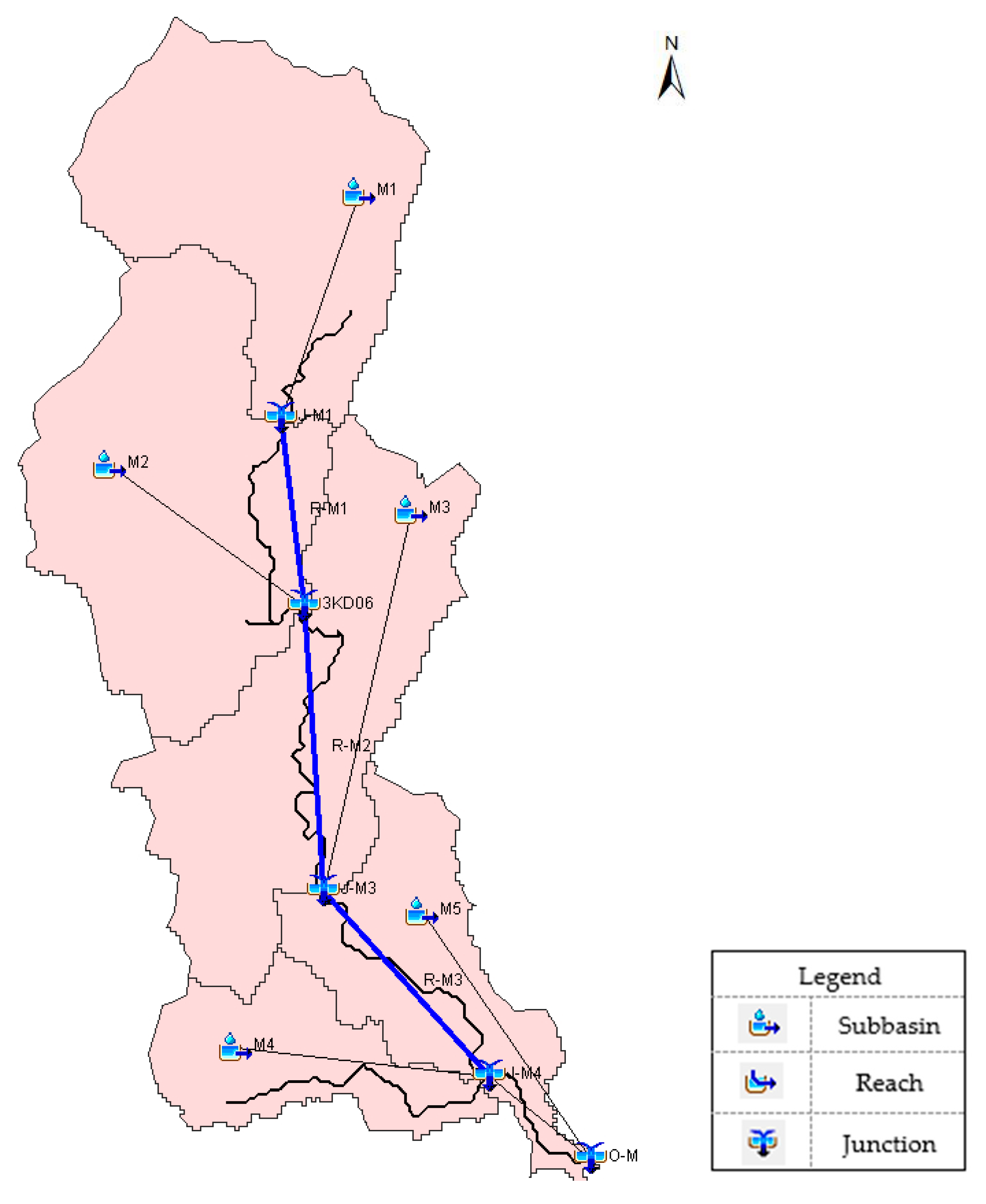
2.5.2. Basin Model Setting-Up in HEC-HMS

For the modeling part, the HEC-HMS [41] was used after calibration, validation and performance evaluation [26]. HEC-HMS is a modeling system which can provide a representation of different watersheds. It simulates the rainfall-runoff processes, producing hydrographs that can be used for further analysis [21].
Before the HEC-HMS project can be run, the following four components are needed: Basin data component, meteorological data component, input data component and control specification component. The basin component is created based on a background map containing the delineated sub-basins derived from the Arc Hydro tool 10.3 from ESRI (Environmental Systems Research Institute). The meteorological component contains the observed precipitation and discharge data; the control specification component determines the simulation period and the time step to be used. The rainfall data (1981–2017) from five rain stations located at the center of each sub-basin and the observed flow (1988–1995) from the stream gauge station (3KD06) were used for the calibration and validation of the model. Due to the location of the 3KD06 station where stream flow data are available, only the two upstream sub-basins—M1 and M2 (Figure 4)—were used. A daily time step was used for the simulation, given the time interval of the available observed data.
All the model setting details are presented in [26] and the user’s manual [21].

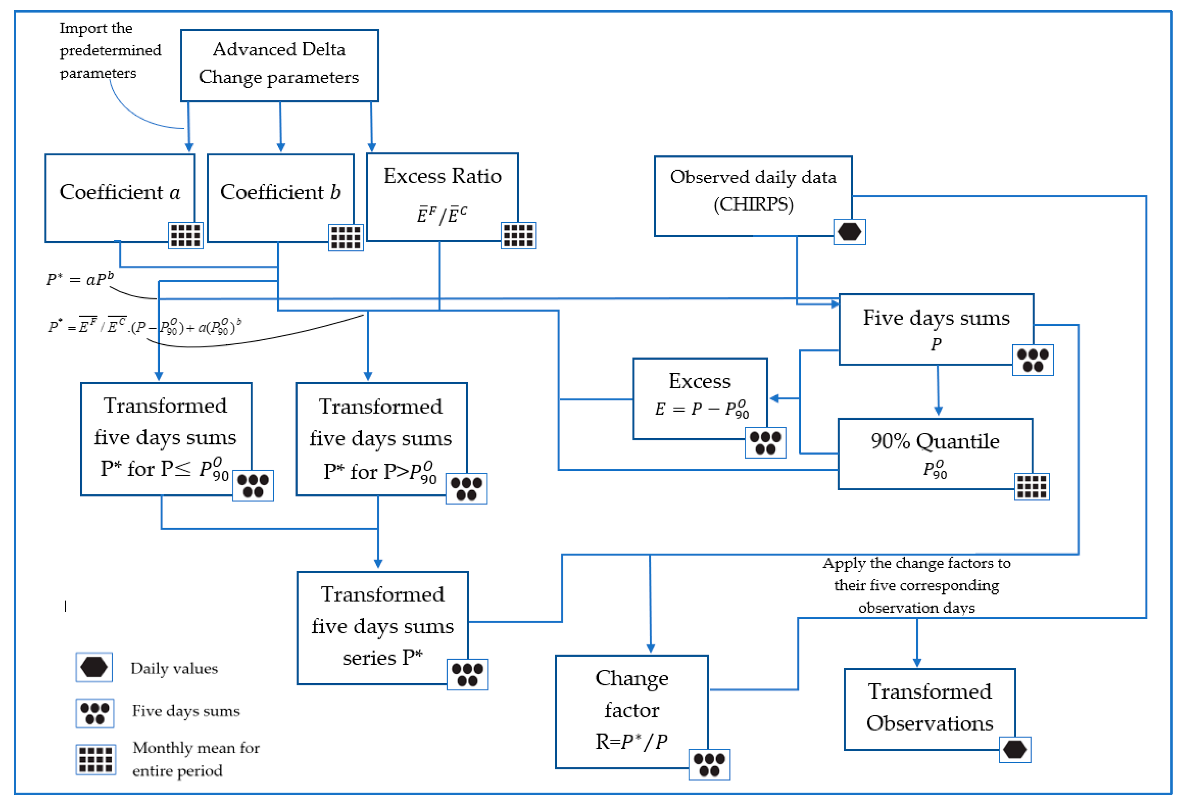
2.5.3. The Advanced Delta Change Approach

The advanced delta change method applied in this study proposed by [34] comprises a non-linear transformation of daily observed precipitation series by using a climate signal from an RCM. The output data were used in the hydrological model to generate flows that were then analyzed to find the impact on flood flow statistics. Rather than a proportional adjustment of observed precipitation, the following non-linear transformation was applied to the data:
P * = a P b
where P and P * represent the observed and future precipitation, respectively, and a and b are the transformation coefficients (a, b > 0).
The coefficients a and b are derived from the 60% quantile ( P 60 ) and the 90% quantile ( P 90 ) of the 5-day precipitation sums and the (future) changes therein. Sample quantiles based on the ordered non-overlapping 5-day precipitation amounts were used as estimates of P 60 and P 90 . The value P 60 was considered because this quantile is closer to the mean than the median value ( P 50 ), owing to the positively skewed probability distribution of the 5-day precipitation amounts. Since the transformation given by Equation (4) represents a monotonic increase, the quantiles of the transformed 5-day precipitation sums are simply obtained by applying the same transformation to the quantiles of the observed 5-day precipitation:
P 60 * = a ( P 60 ) b
P 90 * = a ( P 90 ) b
From these two equations, b is solved by eliminating a and is given by:
b = log ( P 90 * / P 60 * ) log ( P 90 / P 60 )
Once b is determined, a is obtained by substituting b into Equation (5) as:
a = P 60 * / ( P 60 ) b
If there is no bias in the 60 % quantile P 60 C and the 90 % quantile P 90 C in the RCM control simulation compared to the observations, the quantiles P 60 C and P 90 C can be substituted for P 60 and P 90 in Equations (7) and (8), and the quantiles P 60 F and P 90 F in the future climate for P 60 * and P 90 * . The superscripts C and F refer to the control and future simulations, respectively. However, if P 60 and P 90 are biased, this method results in a transformation that does not reproduce the relative changes in these quantiles. In order to ensure that the relative changes of P60 and P90 in the transformed series correspond to the relative changes of these quantiles in the RCM simulation, the following bias-correction factors are introduced:
g 1 = P 60 O / P 60 C
g 2 = P 90 O / P 90 C
where the superscript C again refers to the RCM control climate and O refers to the observed (reference) data. These corrections were applied to P 60 C , P 90 C , P 60 F and P 90 F . The coefficients a and b then become:
b = log { g 2 . P 90 F / g 1 . P 60 F } log { g 2 . P 90 C / g 1 . P 60 C }
a = P 60 F / ( P 60 C ) b . g 1 1 b
Equation (4) can be applied to the observed values for which P P 90 O . For larger P values, this equation is not flexible enough to adequately reproduce the changes in the extremes. This could be improved by separately addressing the change in the excesses, E = P − P90, i.e., the events exceeding P90. The mean excesses for the control and future period are defined as:
E C ¯ =   E C n C   a n d   E F ¯ =   E F n F
where nC and nF are the numbers of 5-day periods in which the 90% quantile is exceeded in the control and future run, respectively. The size of the mean excess is closely related to the slope of an extreme-value plot of the seasonal maximum 5-day precipitation amounts. To ensure that the transformation reproduces the change in the mean excess, Equation (4) becomes [34]:
P * = E F ¯ / E C ¯ . ( P P 90 O ) + a ( P 90 O ) b   f o r   P > P 90 O
Effectively, the excess scales linearly with the factor E F ¯ / E C ¯ . The use of Equation (14) helps to avoid unrealistically high precipitation amounts which may occasionally occur when Equation (4) is used for P > P 90 0 if b > 1.
The final step in the method is to apply a change factor to the daily observation data. The change factor is represented by:
R = P * / P
R for each 5-day sum period, is applied for each day within the 5-day period and is calculated for each station separately. This way, a new precipitation data set is generated for each station. The calculation processes are summarized in Figure 5 and Figure 6.
The output time series from the ADC method were used as input in the HEC-HMS model for modeling the flow. A comparison was then made between the baseline period (1982–2005) and the future period (2018–2041) in order to assess the impact of the ADC method on flow.

2.6. Best-Fit Probability Distribution and Return Period

2.6.1. Best-Fit Probability Distribution

In order to select the distribution that best fits existing data, distributions commonly used in hydrology were tested using a goodness-of-fit test. These included the log normal [43], the log Pearson III [44], the generalized Pareto [44], the generalized extreme values (GEV) [45] and the exponential [45] distributions. Goodness-of-fit test statistics are usually employed to check the validity of a particular probability distribution model on data. In this study the Kolmogorov–Smirnov (K–S) test was used; the K–S test allows for the measurement of the maximum vertical difference between the theoretical ( F x ( x ) ) and empirical ( S n ( x ) ) distributions (this difference is also called the K–S statistic) [46]. The null hypothesis that is being tested is “H0: No difference between observed and expected frequencies”.
Considering a series of n samples, the data are sorted in increasing order ( X 1 < X 2 < < X n ), and the K–S statistic is estimated for each value:
S n ( x ) = 0 ; i f   X = X 1 = k / n ; i f   X k X X k + 1 = 1 ; i f   X > X n
D m a x = m a x | F x ( x ) S n ( x ) |
P ( D m a x D n α ) = 1 α
where D m a x is the absolute maximum difference between observed and expected frequencies, D n α is the critical value (Table A1, Appendix A [47]), α is the significance level, and k is the rank order of the data. H0 is accepted if D m a x D n α .

2.6.2. Return Period of Rainfall and Streamflow

The frequency analysis consisted of the estimation of values of the seasonal maximum rainfall and flow, corresponding to the return periods of 5, 10, 20, 50 years before and after the application of the ADC method. The frequency analysis is employed in hydrology for obtaining a relationship between a particular event and its probability of exceedance. The probability of exceedance can be computed using an empirical or analytical method. A simple empirical method was used and involved sorting the annual series in descending order and assigning an increasing rank to each value.
The maximum 1-day rainfall and flow in the MAMJ (March–April–May–June) and OND (October–November–December) seasons were analyzed in this study, and the empirical return periods were computed using the Weibull plotting position formula given by:
P ( X x ) = m / ( n + 1 ) = 1 F ( x )
T = 1 1 F ( x )
where n is the total number of years and m is the rank of the peak flow values when ranked in descending order; P ( X x ) is the probability of exceedance.
After fitting the data to a distribution, the baseline (1982–2005) return period was estimated for 5, 10, 20, 50 years and then compared with the corresponding return period for the future period (2018–2041). This helped to assess the possible future change in the occurrence of extreme precipitation.

3. Results

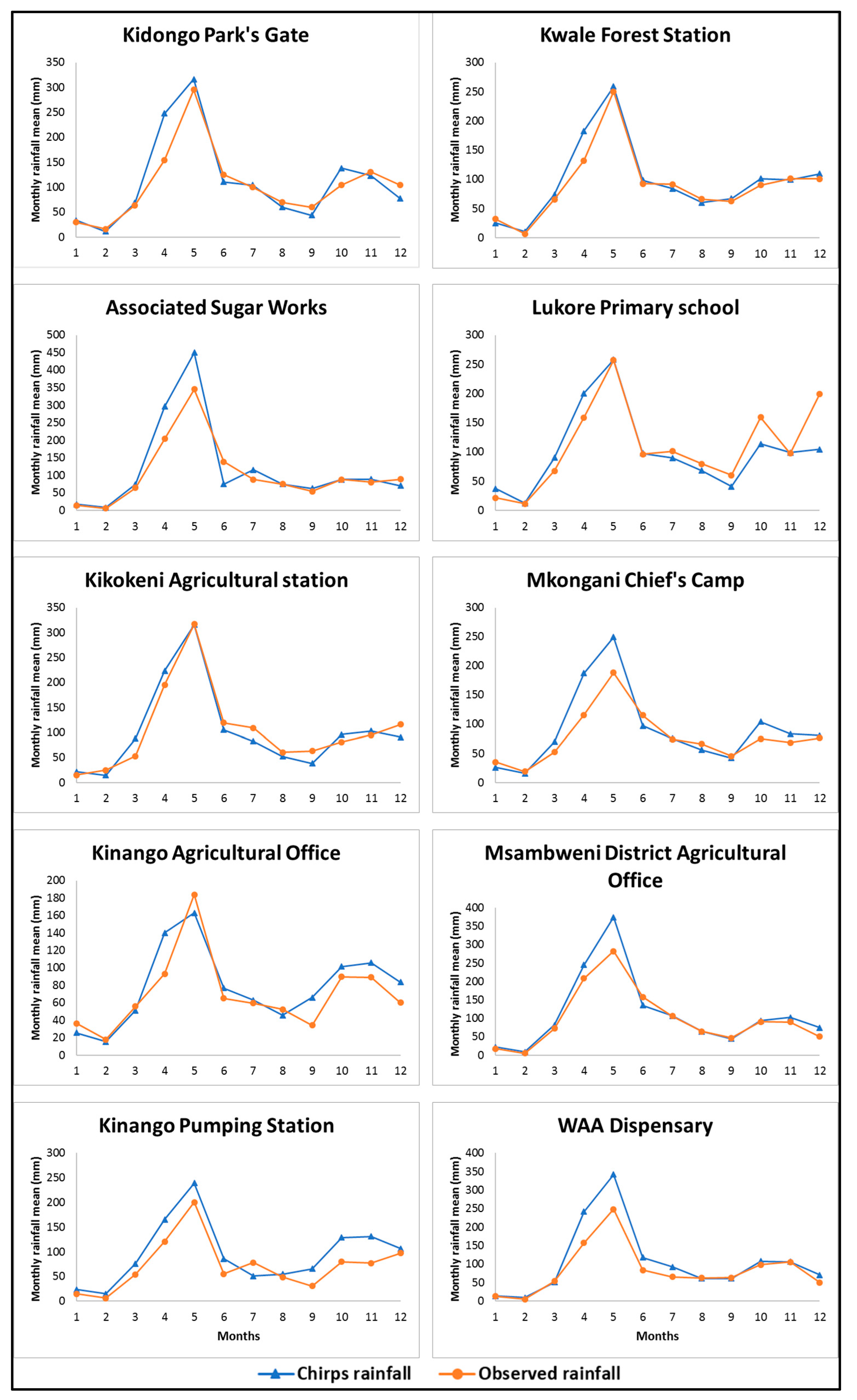
3.1. CHIRPS Datasets Accuracy Analysis

For the satellite-based data accuracy analysis, the comparison was made on monthly and annual totals. Table 3 presents the statistics averaged for each station. The results showed that, on a monthly and an annual basis, all the compared stations had indices of agreement greater than 0.5, which implies that there was a satisfactory degree of agreement between the ground station rainfall and the CHIRPS rainfall. Similarly, all the stations showed good and acceptable correlations on the monthly scale, and only two stations showed a non-satisfactory correlation (R2) on the annual scale. For the absolute error index, on a monthly scale, only two stations showed some high values of RSR and four stations on an annual scale. Globally, the majority of the stations showed acceptable agreement and goodness-of-fit over the years, except for a few years. The months with more than three day gaps were excluded, and this could be the cause of those few disagreements.
Figure 7 represents the graphical comparison of CHIRPS and observed rainfall based on mean monthly distribution. It shows a general agreement and an acceptable fit between CHIRPS and the observed data. These results tie with previous studies [48], wherein CHIRPS products were found to be significantly better than other satellite rainfall data. However, the main limitations of these types of accuracy evaluation are the lack of high-quality data and plausible measurement errors. It is important to highlight the fact that at some of the stations, namely Associated Sugar Works, Mkongani Chief’s Camp, Msambweni District Agricultural Office, Kinango Pumping Station and WAA Dispensary, CHIRPS tended to overestimate the peak rainfall. We speculate that this might be due to the fact that Mkongani Chief’s Camp and WAA Dispensary are located in a bushy environment where some portion of the rainfall could have been stopped by the canopy, therefore occasionally underestimating the rainfall measures. The three other stations with overestimated peaks are located very close to the coast and could have also been subjected to measurement errors due to the high wind speed. Nonetheless, we believe that the satisfactory statistics and graphical agreement on other stations can well justify the fact that CHIRPS rainfall data are a good alternative to low-quality measured data.

3.2. Projection of Future Rainfall Extremes Using the Advanced Delta Change Approach on Regional Climate Models Output

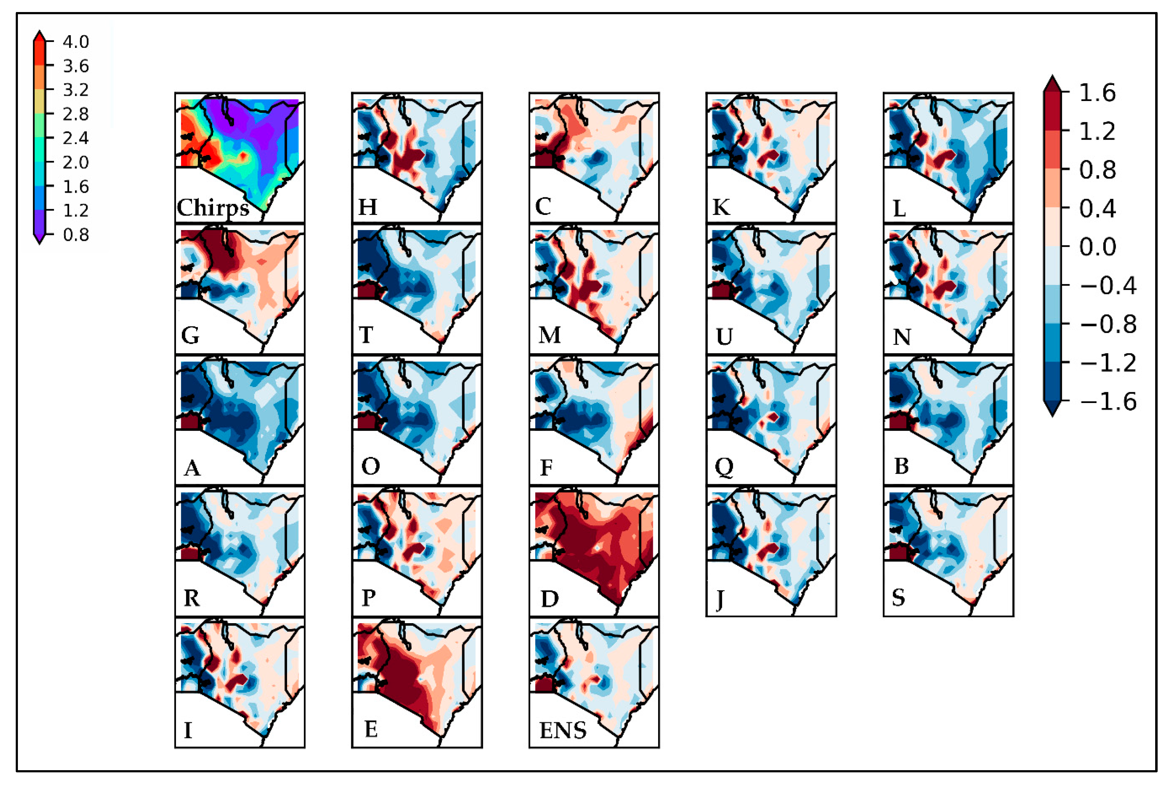
3.2.1. CORDEX Models Performance Evaluation and Selection

Twenty-one models were evaluated against CHIRPS data using RCMES. The models were grouped into five RCMs, each model being forced by different GCMs, as presented in Table 2. The correlation coefficient and the standard deviation were plotted on a Taylor diagram, and the biases were also plotted on maps. Figure 8 represents the bias plot during the studied period (1981–2005). The model bias varied from −1.6 to +1.6 among these RCMs and across the whole country (Kenya). The biases are defined as differences between observations and climate simulations. Two models, namely UQAM-CRCM5 forced by MPI-M-MPI-ESM-LR (D) and UQAM-CRCM5 forced by CCCma-CanESM2 (E) generated an overall high wet bias. Eight models (L, T, U, A, O, Q, F, B and R), however, showed a dry bias in the majority of Kenya. In the South Kenya region particularly, more than half of the RCMs showed a low bias between −0.8 and 0.4. The ensemble, which is an average of all the models, generated the lowest bias all over the area. The values of biases in this study are close to the findings of [49], where biases for Kenya ranged between −2.5 and +2.5.
Figure 9 represents the Taylor diagram analysis of monthly rainfall averaged over Kenya domain during the period 1981–2005, from CHIRPS and the 21 CORDEX models listed in Table 2, with the dashed line representing the reference standard deviation of 1.00. The distance between the reference and individual points corresponds to RMSE [50]. The analysis showed that the spatial pattern of UQAM-CRCM5 model forced by MPI-M-MPI-ESM-LR, and the ensemble closely agreed with CHIRPS, with correlations nearly equal to 0.8. Most RCMs overestimated the extent of the standard deviation. The UQAM-CRCM5 (MPI-M-MPI-ESM-LR) model and ensemble produced a lower RMSE than all RCMs with standard deviations between 1.20 and 1.25. A similar conclusion was reached by [51], who found the UQAM-CRCM5 RCM performed best, and the ensemble mean reproduced the rainfall climatology over Uganda with reasonable skill.

3.2.2. Validation of the Advance Delta Change Model

To project future high rainfall, the advanced delta change method was applied by using models forced by the RCP8.5. As previously described, this approach has the advantage of capturing the extreme wet rainfall. A validation was done to verify if the ADC model was reproducing the observed data well. The method was applied for the ensemble mean of all the RCMs available on RCP8.5, and the time periods that were used are presented in Table 4.
The performance statistics that were used are previously described: RSR, R2 and d. For each station, the statistics were calculated between the transformed and the observed monthly 10%, 30%, 60% and 90% quantiles. The validation results are presented in Table 5. Based on the criteria defined in Table 1, it could be noted that all the five stations were showing acceptable statistics for P 60 and P 90 . For the lower tail of the distribution ( P 10 and P 30 ), the statistics were all acceptable except for M2 and M4. These results are consistent with the fact that the advanced delta change method tend to relatively reproduce the future changes in the upper tail of the distribution as explained by [34]. Based on the model evaluation guideline given by [31], the advanced delta change model was found to have a satisfactory performance. The output was used in the HEC-HMS model for flow modeling before the frequency analysis was performed.

3.2.3. Quantiles Comparison under the Advanced Delta Approach

Table 6 shows the monthly summary of the 10th quantile and the quantile ratios ( P 10 F / P 10 C ) . The analysis showed an increase of the quantiles in the first half of the year (January–July) and a decrease in the last months (August–December). The mean ratios for both periods were numerically close. From January to July, the quantile ratios were P 10 F / P 10 C = 1.2 and P 10 * / P 10 O = 1.1 while from August to December they were P 10 F / P 10 C = P 10 * / P 10 O = 0.8 . However, the individual monthly ratios showed some important differences, especially for February, March and December.
Table 7 shows the monthly summary of the 90th quantile and the quantile ratios ( P 90 F / P 90 C ) . As for the 10th quantile, the analysis showed an increase of the quantiles in the first half part of the year (January–July) and a decrease in the last months (August–December). The mean ratios for both parts were also numerically close; from January to July, P 90 F / P 90 C = 1.1 and P 90 * / P 90 O = 1.2 , while from August to December, P 90 F / P 90 C = P 90 * / P 90 O = 0.8 . However, the individual monthly ratios showed some close values, unlike the 10th quantiles. The correspondence in the monthly quantiles values and the quantiles factors suggests that the ADC transformation emulates the future changes well in these quantiles, with lower differences for the upper tail as found by [34].

3.2.4. Best-Fit Probability Distributions for the Maximum One Day Rainfall in MAMJ and OND Seasons

After applying the K–S test, the best fitting probability distributions were chosen as the ones with the least D m a x , with D m a x D n α : 0.269 for a significance level of 0.05. Having multiple stations and multiple candidate distributions, an average of the maximum distance D m a x was estimated in order to pick the distribution that had the minimal statistic. The results are presented in Table 8, and suggest that for the MAMJ and OND seasons, the generalized Pareto and the exponential distributions can be picked, respectively.

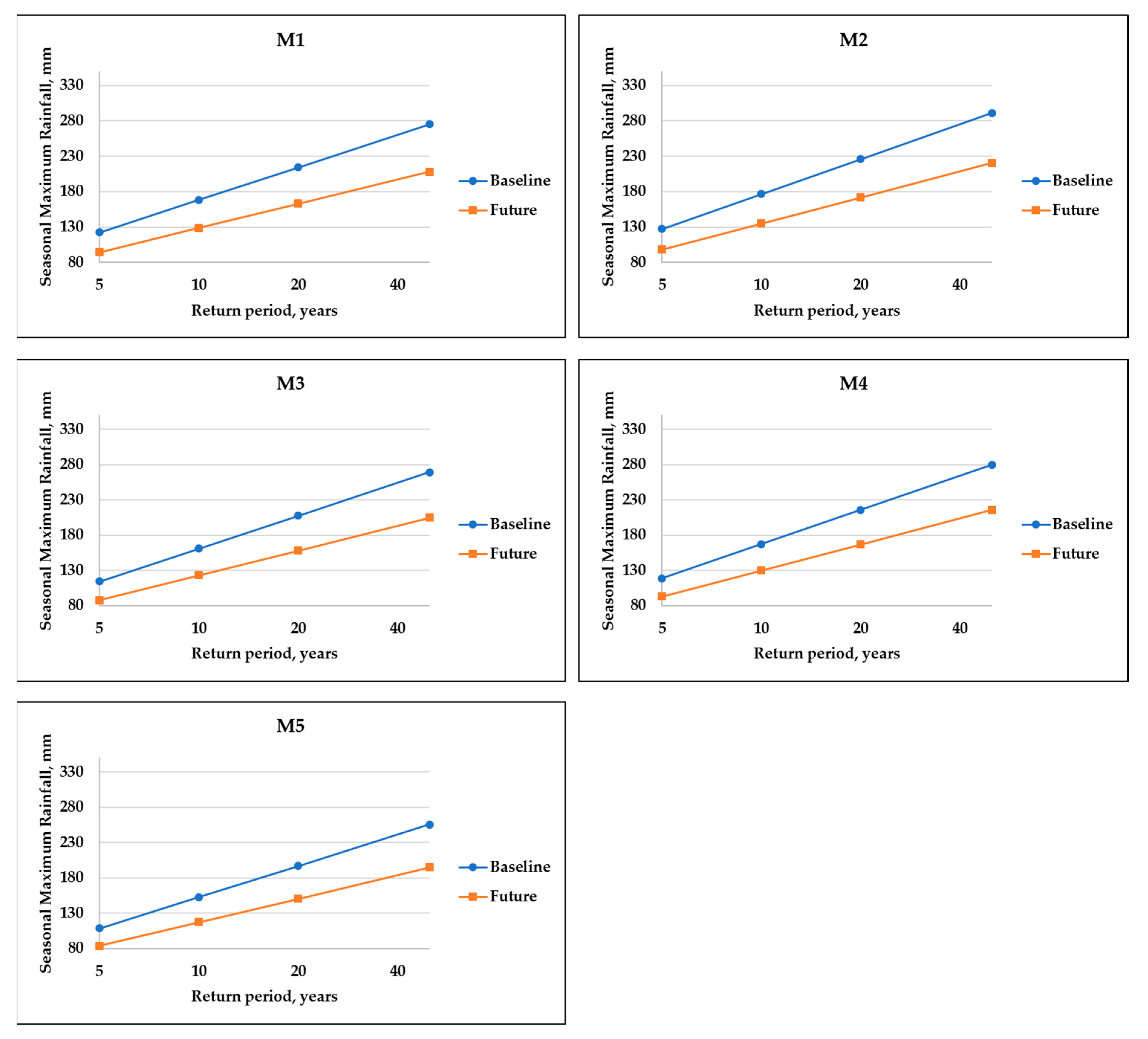
3.2.5. Maximum One Day Rainfall Return Period before and after ADC

The return period of the seasonal maximum rainfall was compared between the observed and the transformed data series, and the plots are presented in Figure 10. The results demonstrated two things. First, all five stations showed an increasing vertical distance between the baseline and the projected maximum rainfall. In fact, from five to 50 years, the vertical distance increased from 15.338, 14.44, 15.445, 15.537, and 15.542 mm to 24.403, 32.809, 32.752, 28.18, and 33.999 mm for sub-basins M1, M2, M3, M4 and M5, respectively. The fact that the values are highly similar for the sub-basins could be explained by their closeness to each other. Second, as previously discussed for the quantiles, it could also be observed that the transformed maximum precipitation was higher than the observed for the MAMJ season.
For example, for M1, a 20-year return period the transformed maximum showed 288.5 mm, while the observed maximum was 267.1 mm. Due to a lack of long-term rainfall data, the researchers decided not to investigate longer return periods because they could significantly be biased.
Figure 11 shows the return period of the seasonal maximum rainfall for the past and transformed data series of October–November–December (OND). As in the MAMJ season, the results indicated that all the five stations showed a similar increasing vertical distance between the baseline and the projected maximum rainfall. In fact, from five to 50 years, the vertical distance increased from 27.968, 29.266, 26.829, 25.892, and 24.937 mm to 66.905, 70.485, 64.507, 63.952, and 60.766 mm for sub-basins M1, M2, M3, M4 and M5, respectively. In this case, again, the values were very similar for the sub-basins, certainly due to their closeness to each other. However, unlike the MAMJ season, the results showed that the observed were much higher than the transformed, which suggested a decrease of the maximum rainfall in the OND season. For example, for M1, a 20-year return period the transformed maximum showed 163.12 mm while the observed maximum was 214.54 mm. These findings suggest that in this part of Kenya (Kwale) the ADC model tends to project an increase in the rainfall wet extremes only in the first rainy season of the year and a decrease in the second rainy season.

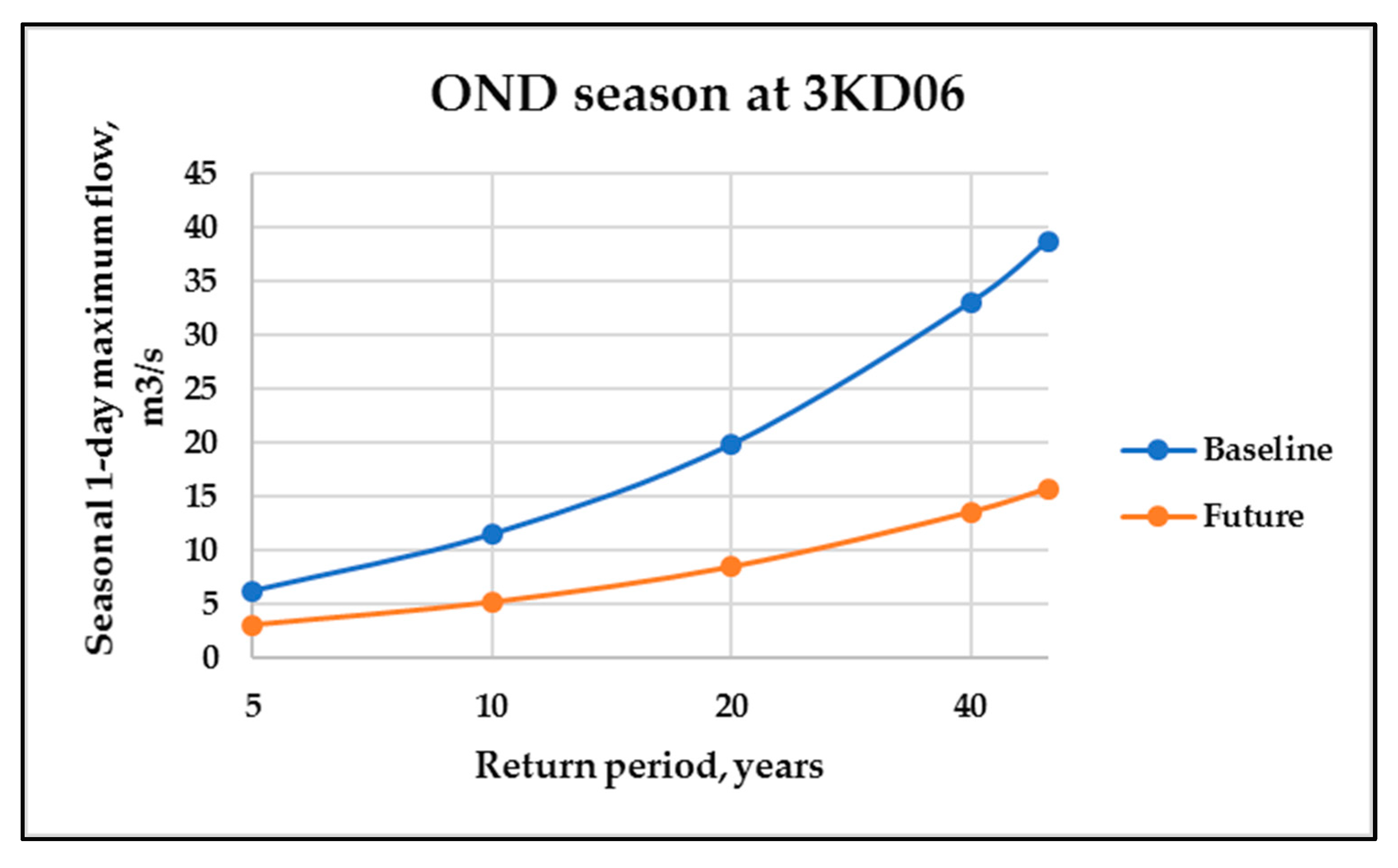
3.3. Hydrological Impact of the Projected Rainfall Extreme on the Gaging Station 3KD06 for the Period 2018–2041

The transformed rainfall data were used as inputs in the HEC-HMS model for evaluating the hydrological response to the projected extreme rainfall. As the observed flow data were available at the 3KD06 gaging station, we decided to assess the changes through the comparison of the observed and the future flow. The MAMJ one day maximum flow was found to fit the exponential distribution well, while the OND one day maximum flow fitted well the Pareto distribution.
Figure 12 shows the MAMJ one day maximum flow return periods for the baseline and the future projection at 3KD06. The results showed an increase in the vertical distance between the baseline and the future. From five to 50 years return period, the vertical distance increased from 6.966 to 14.74 m3/s. As for the MAMJ one day maximum rainfall, the projected stream was higher than the observed streamflow. Another important finding was that for an increase of the 50 year return period maximum rainfall of 24.403 and 32.809 mm at the M1 and M2 sub-basins, respectively, an increase of 14.740 m3/s of the 50-year return period maximum flow was observed at their junction (3KD06).
Figure 13 shows the OND one day maximum flow return periods for the baseline and the future projection at 3KD06. The results showed an increase in the vertical distance between the baseline and the future. From five to 50 years return periods, the vertical distance increased from 3.205 to 22.972 m3/s. As for the OND one day maximum rainfall, the projected stream was lower than the observed streamflow. Another important finding was that for a decrease of the 50-year return period maximum rainfall of 66.905 and 75.485 mm at the M1 and M2 sub-basins, respectively, and a decrease of 22.972 m3/s of the 50-year return period maximum flow, at their junction (3KD06) was observed.

4. Conclusions

In summary, this paper argued that CHIRPS rainfall data were a good alternative to low quality measured data in the studied catchment, and the ensemble of all the models in the historical period generated the lowest bias and the highest correlation all over the area. Additionally, based on the model evaluation guideline given by [31], the advanced delta change (ADC) model was found to have satisfactory performance over the catchment. Moreover, the ADC transformation seemed to have emulated the future changes well in the quantiles and more in reproducing the upper tail of the distribution. The maximum one day rainfall and flow frequency analysis suggested that in the study area, the RCMs bias corrected by the ADC method projected an increase in the rainfall wet extremes in the first rainy season of the year (MAMJ) and a decrease in the second rainy season (OND). These changes in rainfall extremes induced a similar change pattern in streamflow extremes; that is, an increase/decrease of rainfall extremes generated an increase/decrease in streamflow extremes. These results provide evidence in the capability of the ADC bias correction approach to capture the changes in the upper tail of both the rainfall and flow data in the longest and the highest rainy season MAMJ. Future research could further explore peak flow projections for up to 1000 years’ return period if a convenient method is found to generate longer time series of data.

Author Contributions

Conceptualization, W.A.A.O., J.M.G. and J.M.R.; methodology, W.A.A.O., J.M.G. and J.M.R.; validation, W.A.AO., J.M.G. and J.M.R.; writing and original draft preparation, W.A.A.O.; writing, review and editing, J.M.G. and J.M.R.

Funding

This research was funded by the Pan African University of Basic Sciences, Technology and Innovation (PAUSTI).

Acknowledgments

The authors gratefully acknowledge the support of Pan African University of Basic Sciences, Technology and Innovation (PAUSTI), Jomo Kenyatta University of Agriculture and Technology (JKUAT), Kenya Meteorological Department, the Kwale Country Government, Base Titanium Ltd., Kwale International Sugar Company Ltd. and Rural Focus Ltd. This research was co-funded by the UK Government via NERC, ESRC and DFID as part of the Gro for GooD project (UPGro Consortium Grant: NE/M008894/1) and the Pan African University of Basic Sciences, Technology and Innovation (PAUSTI). Special thanks to the Regional Climate Model Evaluation System (RMCES) team, particularly to Huikyo Lee who provides meaningful assistance for adapting the RCMES to CHIRPS and CORDEX-RCMs comparison.

Conflicts of Interest

The authors declare no conflict of interest.

Appendix A

Table A1. Critical values ( D n α ) of the maximum absolute difference between observed and expected frequencies [47].
nSignificance Level, α
0.10.050.020.01
10.950.9750.990.995
20.776390.841890.90.92929
30.636040.70760.784560.829
40.565220.623940.688870.73424
50.509450.563280.627180.66853
60.467990.519260.577410.61661
70.436070.483420.538440.57581
80.409620.454270.506540.54179
90.387460.430010.47960.51332
100.368660.409250.456620.48893
110.352420.391220.43670.4677
120.338150.375430.419180.44905
130.325490.361430.403620.43247
140.314170.34890.38970.41762
150.303970.33760.377130.4042
160.294720.327330.365710.39201
170.286270.317960.355280.38086
180.278510.309360.345690.37062
190.271360.301430.336850.36117
200.264730.294080.328660.35241
210.258580.287240.321040.34427
220.252830.280870.313940.33666
230.247460.27490.307280.32954
240.242420.269310.301040.32286
250.237680.264040.295160.31657
260.23320.259070.289620.31064
270.228980.254380.284380.30502
280.224970.249930.279420.29971
290.221170.245710.274710.29466
300.217560.24170.270230.28987

Appendix B

Figure A1. RCMES workflow for this study (Adapted from [36]).
Hydrology 06 00076 g0a1

References

  1. Boko, M.; Niang, I.; Nyong, A.; Al, E. Climate Change Adaptation and Vulnerability: Contribution of Working Group II to the IV Assessment Report of the IPCC Panel on Climate Change; Cambridge University Press: Cambridge, UK, 2007. [Google Scholar]
  2. Mason, S.J.; Waylen, P.R.; Mimmack, G.M.; Rajaratnam, B.; Harrison, J.M. Changes in extreme rainfall events in South Africa. Clim. Chang. 1999, 41, 249–257. [Google Scholar] [CrossRef]
  3. Fotso-nguemo, T.C.; Chamani, R.; Yepdo, Z.D.; Sonkoué, D.; Matsaguim, C.N.; Vondou, D.A.; Tanessong, R.S. Projected trends of extreme rainfall events from CMIP5 models over Central Africa. Atmos. Sci. Lett. 2018, 19, 1–8. [Google Scholar] [CrossRef]
  4. Ongoma, V.; Chen, H.; Omony, G.W. Variability of Extreme Weather Events over the Equatorial East Africa, a case study of Rainfall in Kenya and Uganda. Theor. Appl. Climatol. 2018, 131, 295–308. [Google Scholar] [CrossRef]
  5. Gebrechorkos, S.H.; Hülsmann, S.; Bernhofer, C. Changes in temperature and precipitation extremes in Ethiopia. Int. J. Climatol. 2018, 39, 18–30. [Google Scholar] [CrossRef]
  6. IPCC. Climate Change 2014: Mitigation of Climate Change. Contribution of Working Group III to the Fifth Assessment Report of the Intergovernmental Panel on Climate Change; Edenhofer, O., Pichs-Madruga, R., Sokona, Y., Farahani, E., Kadner, S., Seyboth, K., Adler, A., Baum, I., Brunner, S., Eickemeier, P., et al., Eds.; Cambridge University Press: Cambridge, UK, 2014. [Google Scholar]
  7. Alotaibi, K.; Ghumman, A.R.; Haider, H.; Ghazaw, Y.M.; Shafiquzzama, M. Future Predictions of Rainfall and Temperature Using GCM and ANN for Arid Regions: A Case Study for the Qassim Region, Saudi Arabia. Water 2018, 10, 1260. [Google Scholar] [CrossRef]
  8. Pisnichenko, I.; Tarasova, T.A. Climate version of the ETA regional forecast model Evaluating. Theor. Appl. Climatol. 2007, 99, 255–272. [Google Scholar] [CrossRef]
  9. Giorgi, F.; Mearns, L.O. Introduction to special section—Regional climate modeling revisited. J. Geophys. Res. 1999, 104, 6335–6352. [Google Scholar] [CrossRef]
  10. Pal, J.S.; Small, E.E.; Eltahir, E.A.B. Simulation of regional-scale water and energy budgets: Representation of subgrid cloud and precipitation processes within RegCM. J. Geophys. Res. 2000, 105, 579–594. [Google Scholar] [CrossRef]
  11. Marinucci, M.R.; Giorgi, F. A 2XCO2 climate change scenario over Europe generated using a limited area model nested in a general Circulation Model 1. Present-Day Seasonal Climate Simulation. J. Geophys. Res. Atmos. 1992, 97, 9989–10009. [Google Scholar] [CrossRef]
  12. USAID. A Review of Downscaling Methods for Climate Change Projections; United States Agency for International Development: Washington, DC, USA, 2014.
  13. Onyutha, C.; Tabari, H.; Rutkowska, A.; Nyeko-ogiramoi, P.; Willems, P. Comparison of different statistical downscaling methods for climate change rainfall projections over the Lake Victoria basin considering CMIP3 and CMIP5. J. Hydro-Environ. Res. 2016, 12, 31–45. [Google Scholar] [CrossRef]
  14. Dee, D.P.; Uppala, S.M.; Simmons, A.J.; Berrisford, P.; Poli, P.; Kobayashi, S.; Andrae, U.; Balmaseda, M.A.; Balsamo, G.; Bauer, P.; et al. The ERA-Interim reanalysis: Configuration and performance of the data assimilation system. Q. J. R. Meteorol. Soc. 2011, 137, 553–597. [Google Scholar] [CrossRef]
  15. Verdin, A.; Rajagopalan, B.; Kleiber, W.; Podestá, G.; Bert, F. A conditional stochastic weather generator for seasonal to multi-decadal simulations. J. Hydrol. 2015, 556, 835–846. [Google Scholar] [CrossRef]
  16. Hay, L.E.; Wilby, R.L.; Leavesley, G.H. A Comparison of Delta Change and Downscaled GCM scenarios for three Mountainous Basins in the United States. J. Am. Water Resour. Assoc. 2000, 36, 387–397. [Google Scholar] [CrossRef]
  17. Graham, L.P.; Andréasson, J.; Carlsson, B. Assessing climate change impacts on hydrology from an ensemble of regional climate models, model scales and linking methods—A case on the Lule River basin. Clim. Chang. 2007, 81, 293–307. [Google Scholar] [CrossRef]
  18. Bordoy, R.; Burlando, P. Bias correction of regional climate model simulations in a region of complex orography. J. Appl. Meteorol. Climatol. 2013, 52, 82–101. [Google Scholar] [CrossRef]
  19. Leander, R.; Buishand, T.A. Resampling of regional climate model output for the simulation of extreme river flows. J. Hydrol. 2007, 332, 487–496. [Google Scholar] [CrossRef]
  20. Teutschbein, C.; Seibert, J. Is bias correction of regional climate model (RCM) simulations possible for non-stationary conditions? Hydrol. Earth Syst. Sci. 2013, 17, 5061–5077. [Google Scholar] [CrossRef] [Green Version]
  21. Scharffenberg, W.A. Hydrologic Modeling System HEC-HMS—User’s Manual (ver. 4.0); USACE: Davis, CA, USA, 2013.
  22. Rehana, S.; Mujumdar, P.P. River water quality response under hypothetical climate change scenarios in Tunga-Bhadra river, India. Hydrol. Process. 2011, 25, 3373–3386. [Google Scholar] [CrossRef] [Green Version]
  23. Tefera, A.H. Application of water balance model simulation for water resource assessment in upper Blue Nile of North Ethiopia using HEC-HMS by GIS and remote sensing: Case of Beles river basin. Int. J. Hydrol. 2017, 1, 222–227. [Google Scholar] [CrossRef]
  24. Muli, N.M. Rainfall-Runoff Flood Modelling in Nairobi Urban Watershed. Master’s Thesis, Kenyatta University, Nairobi, Kenya, 2011. [Google Scholar]
  25. Bitew, G.T.; Mulugeta, A.B.; Miegel, K. Application of HEC-HMS Model for Flow Simulation in the Lake Tana Basin: The Case of Gilgel Abay Catchment, Upper Blue Nile Basin, Ethiopia. Hydrology 2019, 6, 1–17. [Google Scholar]
  26. Ouédraogo, W.A.A.; Raude, J.M.; Gathenya, M.J. Continuous Modeling of the Mkurumudzi River Catchment in Kenya Using the HEC-HMS Conceptual Model: Calibration, Validation, Model Performance Evaluation and Sensitivity Analysis. Hydrol. Sci. J. 2018, 5, 44. [Google Scholar] [CrossRef]
  27. Katuva, J.M. Water Allocation Assessment: A Study of Hydrological Simulation on Mkurumudzi River Basin. Ph.D. Thesis, University of Nairobi, Nairobi, Kenya, 2014. [Google Scholar]
  28. Funk, C.; Peterson, P.; Landsfeld, M.; Pedreros, D.; Verdin, J.; Shukla, S.; Husak, G.; Rowland, J.; Harrison, L.; Hoell, A.; et al. The climate hazards infrared precipitation with stations—A new environmental record for monitoring extremes. Sci. Data 2015, 2, 1–21. [Google Scholar] [CrossRef]
  29. Yared, B.; Tsegaye, T.; Getachew, D.; Andualem, S. Evaluation of Satellite-Based Rainfall Estimates and Application to Monitor Meteorological Drought for the Upper Blue Nile Basin, Ethiopia. Remote Sens. 2017, 9, 669. [Google Scholar] [Green Version]
  30. Legates, D.R.; Mccabe, G.J. Evaluating the Use Of “Goodness-of-Fit” Measures in Hydrologic and Hydroclimatic Model Validation Evaluating the use of “goodness-of-fit” measures in hydrologic and hydroclimatic model validation. Water Resour. Res. 1999, 35, 233–241. [Google Scholar] [CrossRef]
  31. Moriasi, D.N.; Arnold, J.G.; Van Liew, M.W.; Bingner, R.L.; Harmel, R.D.; Veith, T.L. Model Evaluation Guidelines for Systematic Quantification of Accuracy in Watershed Simulations. ASABE 2007, 50, 885–900. [Google Scholar] [CrossRef]
  32. Willmott, C.J. On the validation of Models. Phys. Geogr. 2013, 37–41. [Google Scholar] [CrossRef]
  33. Santhi, C.; Arnold, J.G.; Williams, J.R.; Dugas, W.A.; Srinivasan, R.; Hauck, L.M. Validation of the SWAT model on a large river basin with point and nonpoint sources. J. Am. Water Resour. Assoc. 2002, 37, 1169–1188. [Google Scholar] [CrossRef]
  34. Van Pelt, S.C.; Beersma, J.J.; Buishand, T.A.; van den Hurk, B.J.J.M.; Kabat, P. Future changes in extreme precipitation in the Rhine basin based on global and regional climate model simulations. Hydrol. Earth Syst. Sci. 2012, 16, 4517–4530. [Google Scholar] [CrossRef] [Green Version]
  35. Lee, H.; Goodman, A.; Mcgibbney, L.; Waliser, D.E.; Kim, J.; Loikith, P.C.; Gibson, P.B.; Massoud, E.C. Regional Climate Model Evaluation System powered by Apache Open Climate Workbench v1. 3.0: An enabling tool for facilitating regional climate studies. Geosci. Model Dev. 2018, 11, 4435–4449. [Google Scholar] [CrossRef]
  36. Waliser, D.E.; Kyo, L.; Goodman, A.; Wilson, B.; Loikith, P.; Gibson, P.B.; Massoud, E.C.; Zimdars, P.A. Tutorials Overview: Regional Climate Model Evaluation System. Available online: https://rcmes.jpl.nasa.gov/content/tutorials-overview (accessed on 31 January 2019).
  37. Riahi, K.; Grübler, A.; Nakicenovic, N. Scenarios of long-term socio-economic and environmental development under climate stabilization. Technol. Forecast. Soc. Chang. 2007, 74, 887–935. [Google Scholar] [CrossRef]
  38. Masui, T.; Matsumoto, K.; Hijioka, Y.; Kinoshita, T.; Nozawa, T.; Ishiwatari, S.; Kato, E.; Shukla, P.R.; Yamagata, Y.; Kainuma, M. An emission pathway to stabilize at 6 W/m2 of radiative forcing. Clim. Chang. Chang. 2011. [Google Scholar] [CrossRef]
  39. Thomson, A.M.; Calvin, K.V.; Smith, S.J.; Kyle, G.P.; Volke, A.; Patel, P.; Delgado-Arias, S.; Bond-Lamberty, B.; Wise, M.A.; Clarke, L.E. RCP4.5: A pathway for stabilization of radiative forcing by 2100. Clim. Chang. 2011, 109, 77. [Google Scholar] [CrossRef]
  40. Van Vuuren, D.P.; Stehfest, E.; Den Elzen, M.G.J.; Deetman, S.; Hof, A.; Isaac, M.; Klein Goldewijk, K.; Kram, T.; Mendoza Beltran, A.; Oostenrijk, R. RCP2.6: Exploring the possibility to keep global mean temperature change below 2 °C. Clim. Chang. 2011, 109, 95. [Google Scholar] [CrossRef]
  41. Feldman, A.D. Hydrologic modeling system HEC-HMS, Technical Reference Manual. Tech. Ref. Man. 2000, 145. [Google Scholar]
  42. Kraaijenbrink, P. Advanced Delta Change Method: Extension of an Application to CMIP5 GCMs; KNMI: De Bilt, The Netherlands, 2013. [Google Scholar]
  43. Markovic, R.D. Probability Functions of Best Fit to Distributions of Annual Precipitation and Runoff. In Colorado State University Hydrology Paper No. 8; Colorado State University: Fort Collins, CO, USA, 1965. [Google Scholar]
  44. Alam, A.A.; Emura, K.; Farnham, C.; Yuan, J. Best-Fit Probability Distributions and Return Periods for Maximum Monthly Rainfall in Bangladesh. Climate 2018, 6, 9. [Google Scholar] [CrossRef]
  45. Hosking, J.R.M.; Allis, J.R. Regional Frequency Analysis: An Approach Based on L-Moments, 1st ed.; Cambridge University Press: Cambridge, UK, 1997; ISBN 978-0-521-43045-6. [Google Scholar]
  46. Conover, W.J. Practical Nonparametric Statistics, 3rd ed.; JohnWiley & Sons, Inc.: New York, NY, USA, 1999; ISBN 0471160687. [Google Scholar]
  47. O’Connor, P.D.T.; Kleyner, A. Appendix 3 Kolmogorov—Smirnov Tables. In Practical Reliability Engineering; John Wiley & Sons, Inc.: New York, NY, USA, 2012; pp. 455–456. [Google Scholar]
  48. Dinku, T.; Funk, C.; Peterson, P.; Maidment, R.; Tadesse, T.; Gadain, H.; Ceccato, P. Validation of the CHIRPS satellite rainfall estimates over eastern Africa. Q. J. R. Meteorol. Soc. 2018, 144, 292–312. [Google Scholar] [CrossRef] [Green Version]
  49. Kim, J.; Waliser, D.E.; Mattmann, C.A.; Goodale, C.E.; Hart, A.F.; Zimdars, P.A.; Crichton, D.J.; Jones, C.; Nikulin, G.; Hewitson, B.; et al. Evaluation of the CORDEX-Afrcia multi-RCM hindcast: Systematic model errors. Clim. Dyn. 2013, 42, 1189–1202. [Google Scholar] [CrossRef]
  50. Taylor, K.E. Summarizing multiple aspects of model performance in a single diagram. J. Geophys. Res. 2001, 106, 7183–7192. [Google Scholar] [CrossRef]
  51. Kisembe, J.; Favre, A.; Dosio, A.; Lennard, C.; Sabiiti, G.; Nimusiima, A. Evaluation of rainfall simulations over Uganda in CORDEX regional climate models. Theor. Appl. Climatol. 2018, 1–19. [Google Scholar] [CrossRef]
Figure 1. Location Map of Mkurumudzi catchment within Kwale County in Kenya.
Hydrology 06 00076 g001
Figure 2. Methodology flow chart.
Hydrology 06 00076 g002
Figure 3. Rainfall stations data availability graph (Source: Kenya Meteorological Department).
Hydrology 06 00076 g003
Figure 4. Mkurumudzi basin model (Source [26]).
Hydrology 06 00076 g004
Figure 5. Flowchart of the parameter calculation steps of the advanced delta change method (adapted from [42]).
Hydrology 06 00076 g005
Figure 6. Flowchart of the transformation of the observation time series, or application of the coefficients (adapted from [42]).
Hydrology 06 00076 g006
Figure 7. Comparison of CHIRPS and observed rainfall based on mean monthly distribution.
Hydrology 06 00076 g007
Figure 8. Bias plot of the observation against individual model: [The letters A to U represent the models’ IDs referred in Table 2).
Hydrology 06 00076 g008
Figure 9. Taylor diagram analysis of monthly rainfall averaged over Kenya domain during the period 1981–2005, from CHIRPS and the 21 Coordinated Regional Climate Downscaling Experiment (CORDEX) models listed in Table 2.
Hydrology 06 00076 g009
Figure 10. Return periods comparison of the maximum one day rainfall for MAMJ season.
Hydrology 06 00076 g010
Figure 11. Return periods comparison of the maximum one day rainfall for OND season.
Hydrology 06 00076 g011
Figure 12. Return periods comparison of the maximum one day flow for MAMJ season.
Hydrology 06 00076 g012
Figure 13. Return periods comparison of the maximum one day flow for OND season.
Hydrology 06 00076 g013
Table 1. General performance ratings for recommended statistics [31].
No.Performance RatingR2dRSR
1Very Good0.75 to 10.90 to 10 to 0.50
2Good0.65 to 0.750.75 to 0.900.50 to 0.60
3Satisfactory0.50 to 0.650.50 to 0.750.60 to 0.70
4Unsatisfactory<0.50<0.50>0.70
Table 2. List of the regional climate models that were evaluated in this study.
RCMsInstituteDriving GCMsID
CLMcom-CCLM4-8-17Climate Limited-area Modelling Community (CLM-Community), GermanyMOHC-HadGEM2-ESA
MPI-M-MPI-ESM-LRB
CNRM-CERFACS-CNRM-CM5C
UQAM-CRCM5Universite du Québec à Montréal, CanadaMPI-M-MPI-ESM-LRD
CCCma-CanESM2E
KNMI-RACMO22TRoyal Netherlands Meteorological Institute, De Bilt, The NetherlandsMOHC-HadGEM2-ESF
ICHEC-EC-EARTHG
SMHI-RCA4Swedish Meteorological and Hydrological Institute, Rossby CentreCCCma-CanESM2H
NOAA-GFDL-GFDL-ESM2MI
NCC-NorESM1-MJ
CNRM-CERFACS-CNRM-CM5K
CSIRO-QCCCE-CSIRO-Mk3-6-0L
IPSL-IPSL-CM5A-MRM
MIROC-MIROC5N
MOHC-HadGEM2-ESO
MPI-M-MPI-ESM-LRP
GERICS-REMO2009Helmholtz-Zentrum Geesthacht, Climate Service Center Germany, Alfred Wegener Institute, Helmholtz Centre for Polar and Marine Research, GermanyMOHC-HadGEM2-ESQ
MPI-M-MPI-ESM-LRR
NOAA-GFDL-GFDL-ESM2GS
IPSL-IPSL-CM5A-LRT
MIROC-MIROC5U
Table 3. Computed statistics of goodness-of-fit between observed and Climate Hazards Group InfraRed Precipitation with Station (CHIRPS) rainfall data for ten stations and for the period 1981–2016.
12345678910
Monthly scale
R20.640.790.810.760.770.560.580.670.730.68
d0.840.910.860.890.930.810.890.870.880.88
RSR0.490.500.921.010.490.740.570.620.560.55
Annual scale
R20.620.610.290.880.70.180.770.770.720.77
d0.860.840.540.940.890.550.920.90.80.83
RSR0.690.770.990.420.561.170.520.590.910.82
*Corresponding Stations’ NamesKidongo Park’s GateKwale Forest StationAssociated Sugar worksLukore Primary schoolKikokeni Agricultural stationMkongani Chief’s CampKinango Agricultural OfficeMsambweni Agricultural OfficeKinango Pumping stationWAA Dispensary
Table 4. Rainfall data period spans used in the advance delta change model.
Rainfall Data PeriodsStart Year–End Year
Observed period1982–1992
Control period1982–1992
Validation period2006–2016
Observed period for validation2006–2016
Table 5. Advanced delta change model validation results.
StationsStatisticsP10P30P60P90
M1RSR0.70.60.70.7
R20.60.70.60.7
d0.90.90.90.9
M2RSR0.90.70.60.7
R20.30.60.70.7
d0.70.90.90.9
M3RSR0.60.40.50.7
R20.60.80.80.7
d0.91.00.90.9
M4RSR1.11.00.60.7
R20.30.60.80.7
d0.70.80.90.9
M5RSR0.70.40.50.7
R20.60.90.80.7
d0.91.01.00.9
Table 6. Monthly summary of 10% quantiles and quantile ratios averaged for all stations.
P 10 C P 10 F Ratio P 10 O P 10 * Ratio
Control Series (mm)Future Series (mm) Observed Series (mm) Transformed Series (mm)
Months(1982–2005)(2018–2041)(1982–2005)(2018–2041)
January4.44.41.00.40.31.0
February3.65.21.40.00.01.0
March6.19.51.60.30.41.3
April17.419.11.16.27.21.2
May18.622.11.23.33.81.2
June10.711.81.15.56.41.2
July7.88.41.12.62.71.1
Average9.811.51.22.63.01.1
August7.66.90.90.90.80.8
September9.37.00.80.50.40.7
October15.111.50.80.60.40.8
November16.112.40.82.42.00.8
December8.06.00.70.20.20.9
Average11.28.80.80.90.70.8
Table 7. Monthly summary of 90% quantiles and quantile ratios averaged for all stations.
P 90 C P 90 F Ratio P 90 O P 90 * Ratio
Control Series Future Series Observed Series Transformed Series
Months(1982–2005)(2018–2041)(1982–2005)(2018–2041)
January12.812.71.010.512.61.2
February11.416.81.56.710.01.5
March18.623.31.330.136.51.2
April38.640.91.185.793.61.1
May40.445.11.1149.1161.41.1
June27.528.41.044.447.61.1
July18.720.01.135.232.30.9
Average24.026.71.151.756.31.2
August19.217.60.924.820.30.8
September24.818.40.717.112.40.7
October37.526.20.740.028.20.7
November32.228.40.944.035.90.8
December23.716.80.732.929.00.9
Average27.421.50.831.825.20.8
Table 8. Best-fitting distributions for the maximum one day rainfall in March–April–May–June (MAMJ) and October–November–December (OND) seasons for each station.
SeasonsDistributionsM1M2M3M4M5Average Dmax
D m a x p-Value D m a x p-Value D m a x p-Value D m a x p-value D m a x p-Value
MAMJLogNormal0.0790.990.0631.000.0920.960.0970.940.0840.980.083
Log Pearson III0.0711.000.0591.000.0830.980.0790.990.0711.000.073
GEV-Max (L-moments)0.0840.980.0581.000.0850.980.0780.990.0760.990.076
Pareto (L-moments)0.0741.000.0571.000.0880.970.0601.000.0671.000.069
ONDExponential (L-moments)0.0721.000.0671.000.0750.990.0890.970.0930.960.079
Log Pearson III0.0810.990.0840.980.0840.980.0930.960.1000.930.09
Pareto (L-moments)0.0721.000.0671.000.0770.990.0880.970.0970.950.080

