Calibration and Validation of the Cosmic Ray Neutron Rover for Soil Water Mapping within Two South African Land Classes

Abstract
1. Introduction
2. Methodology
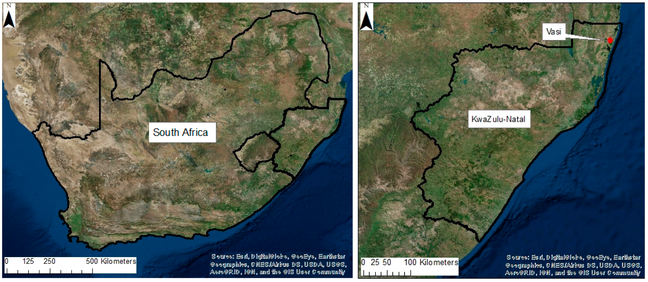
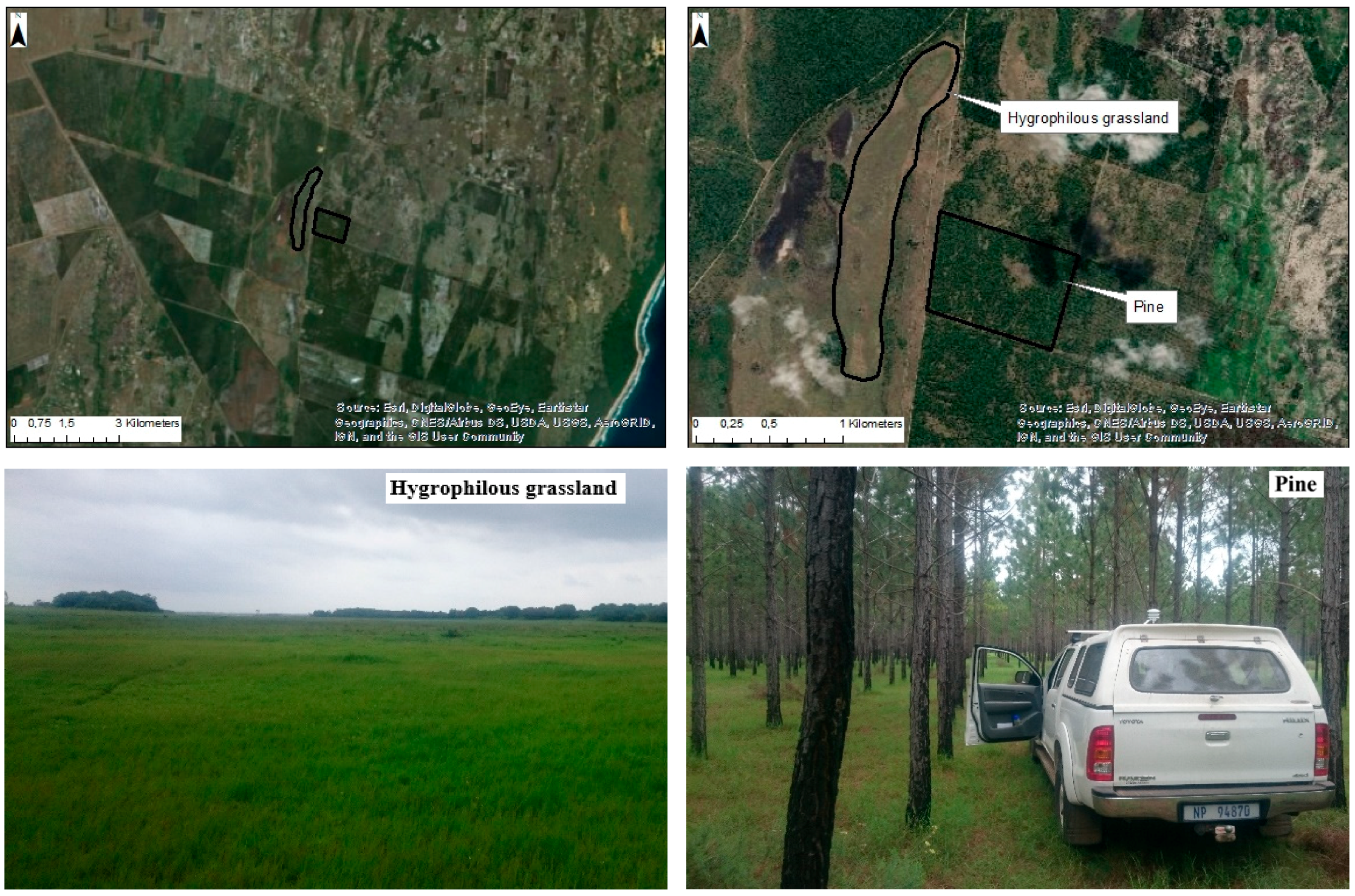
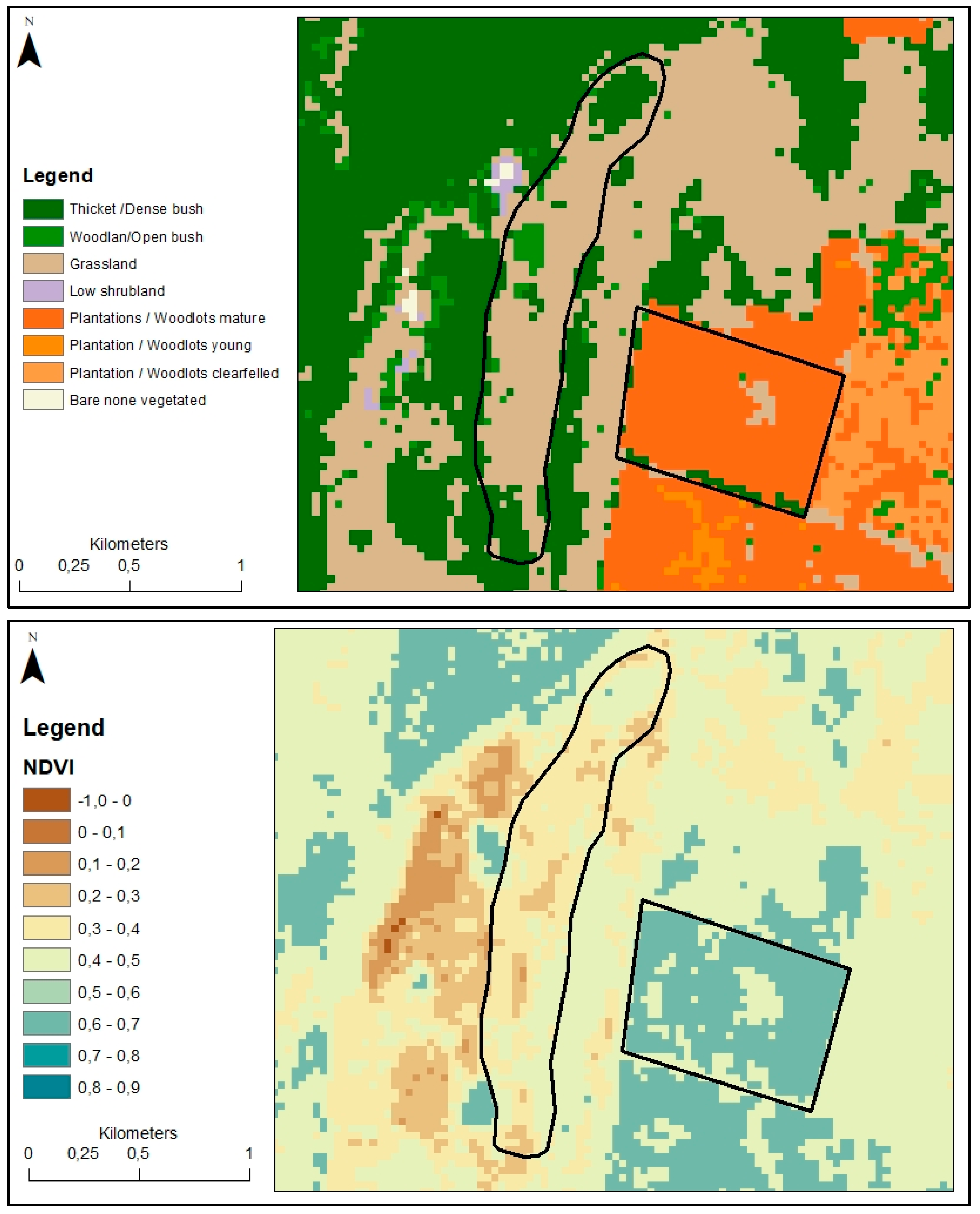
2.1. Study Site
2.2. Cosmic Ray Neutron Method
2.3. Cosmic Ray Neutron Rover System
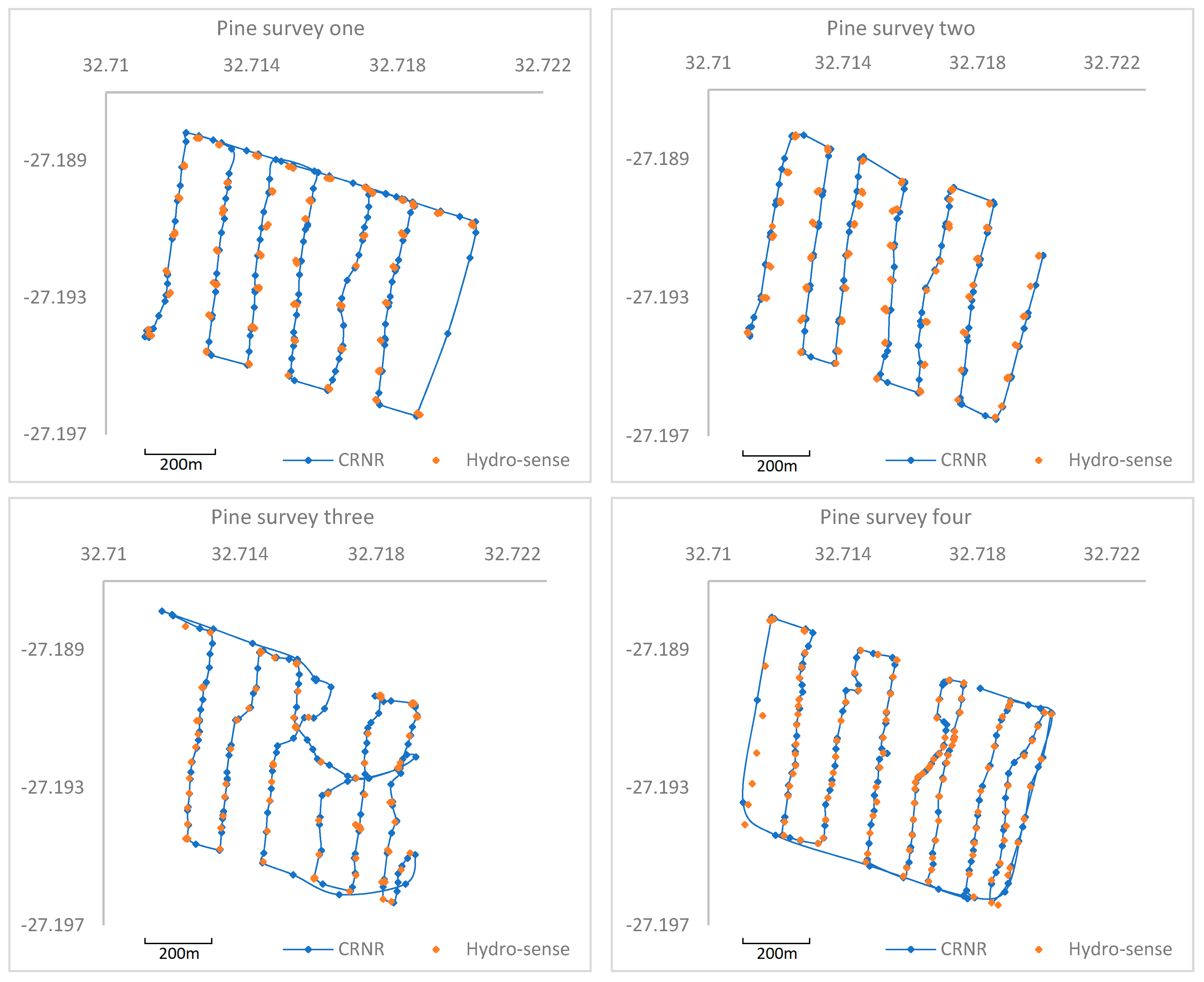
2.4. Cosmic Ray Neutron Rover Surveys
2.5. Neutron Correction Factors
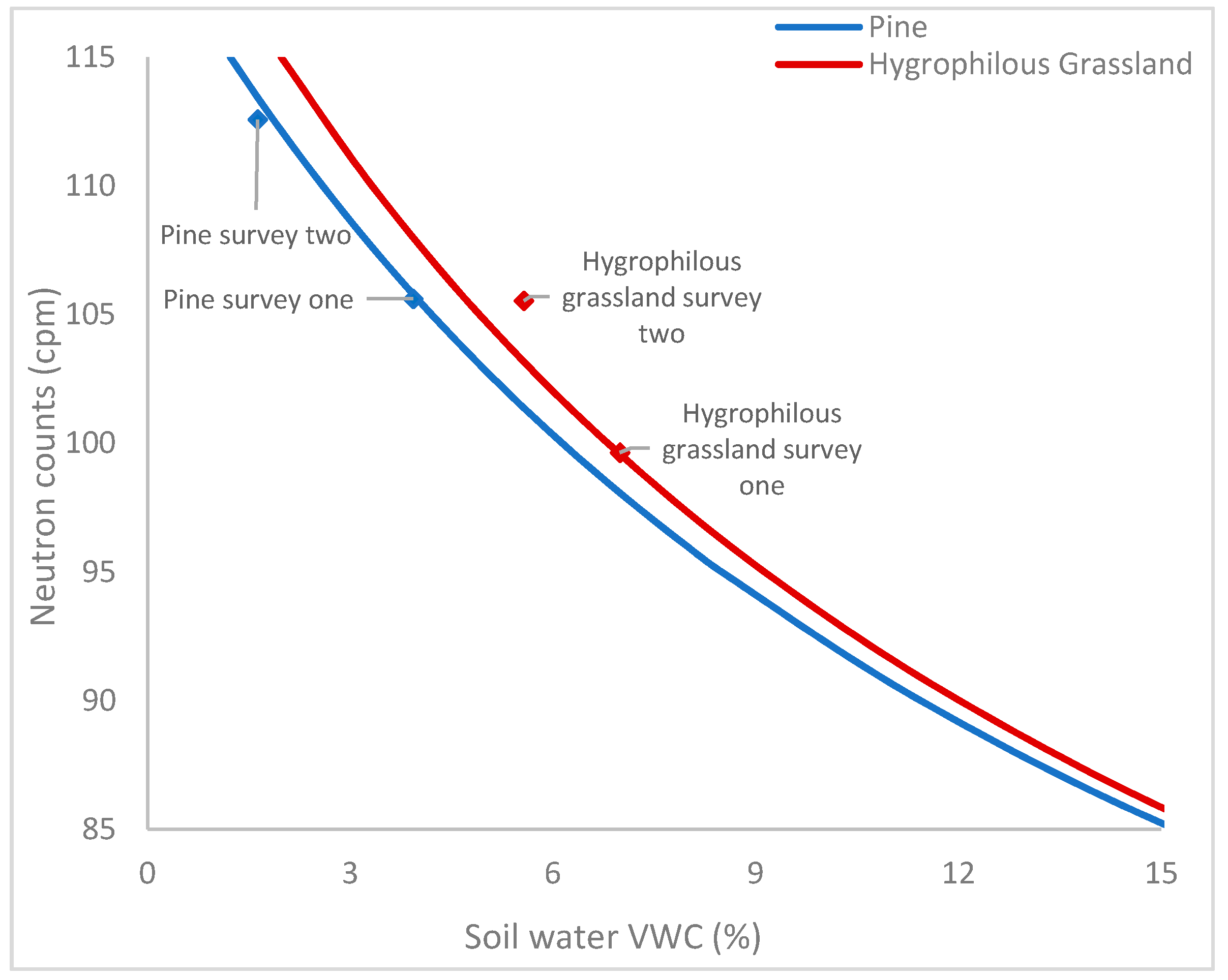
2.6. Calibration
3. Results
3.1. Calibration Assessment
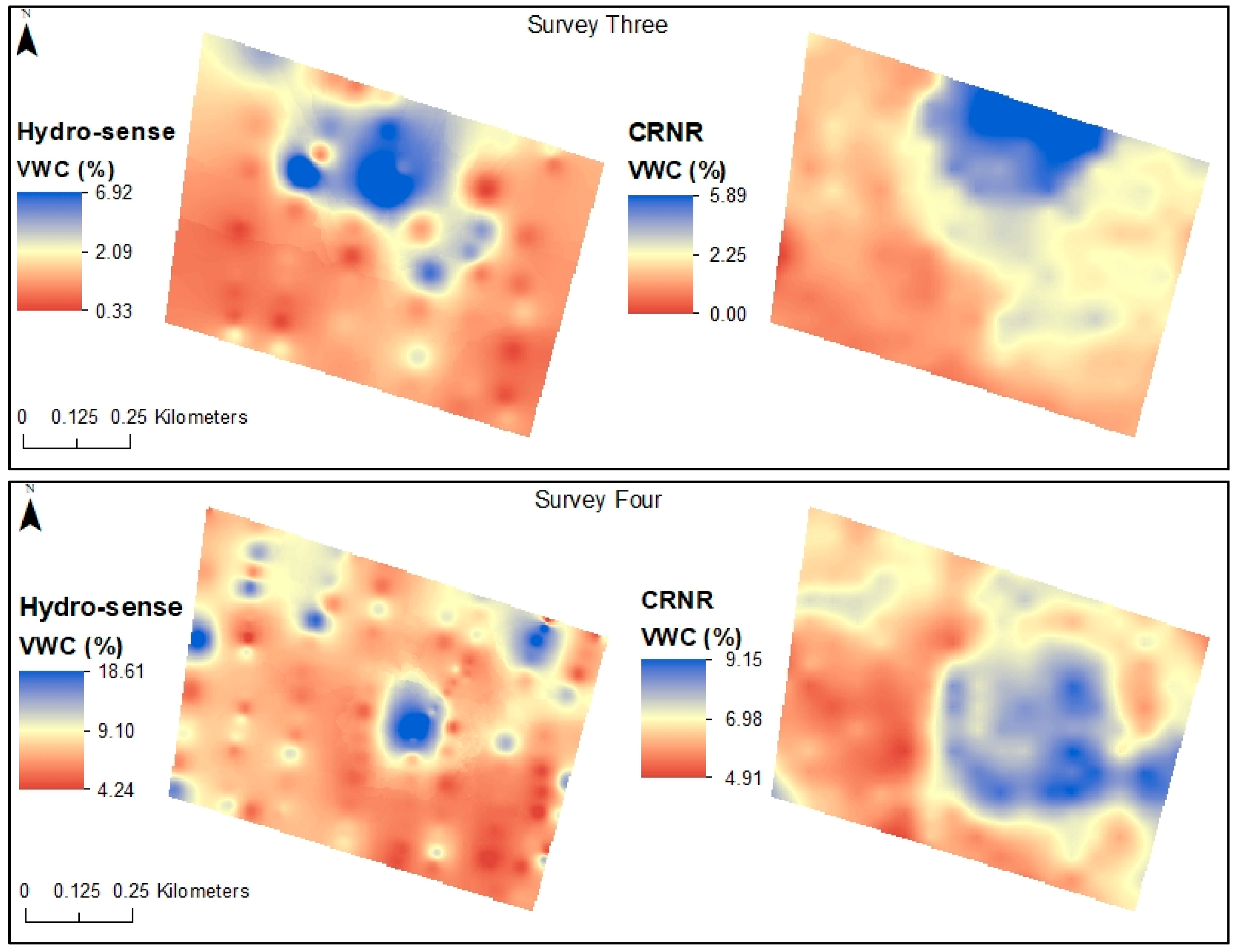
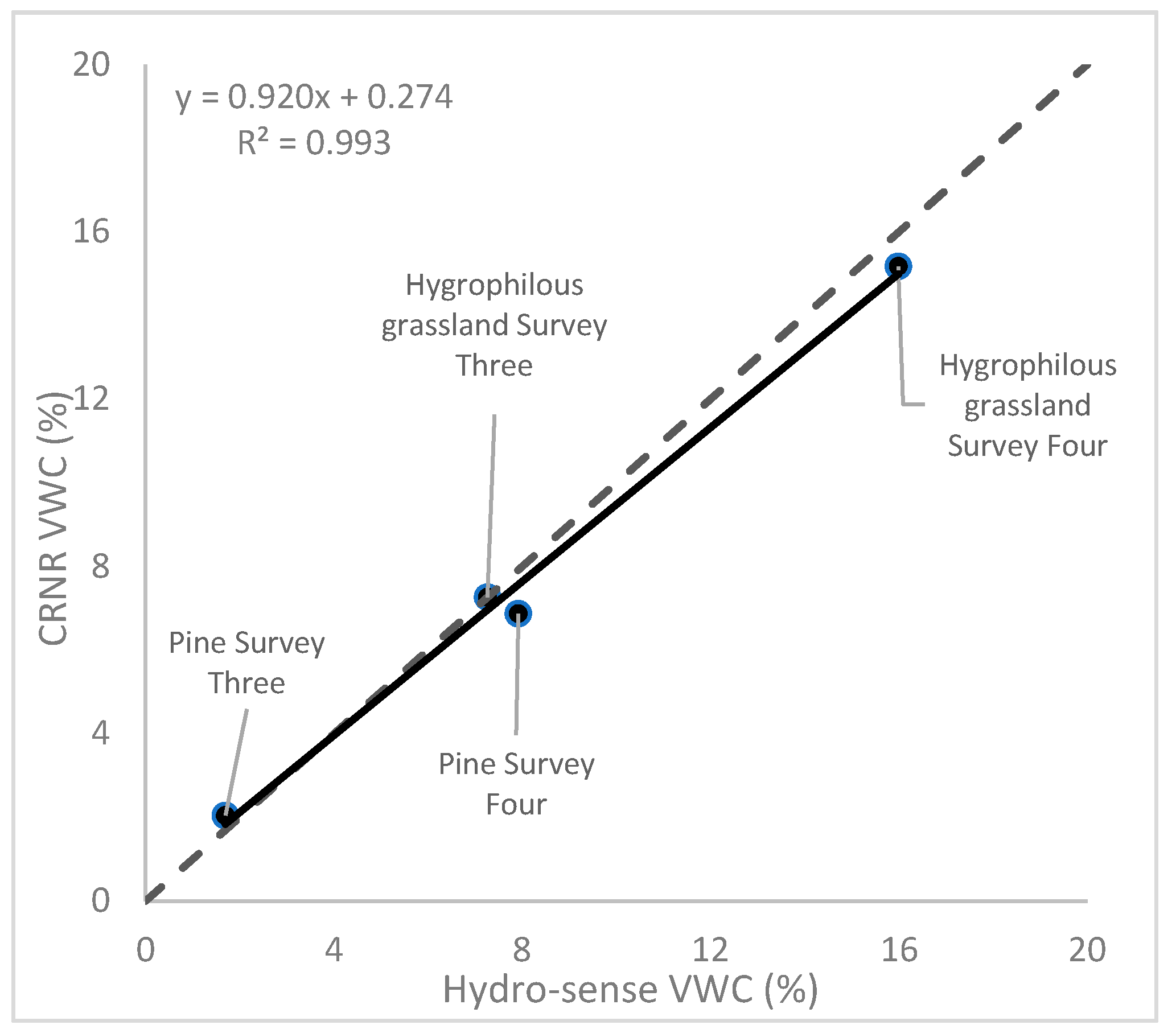
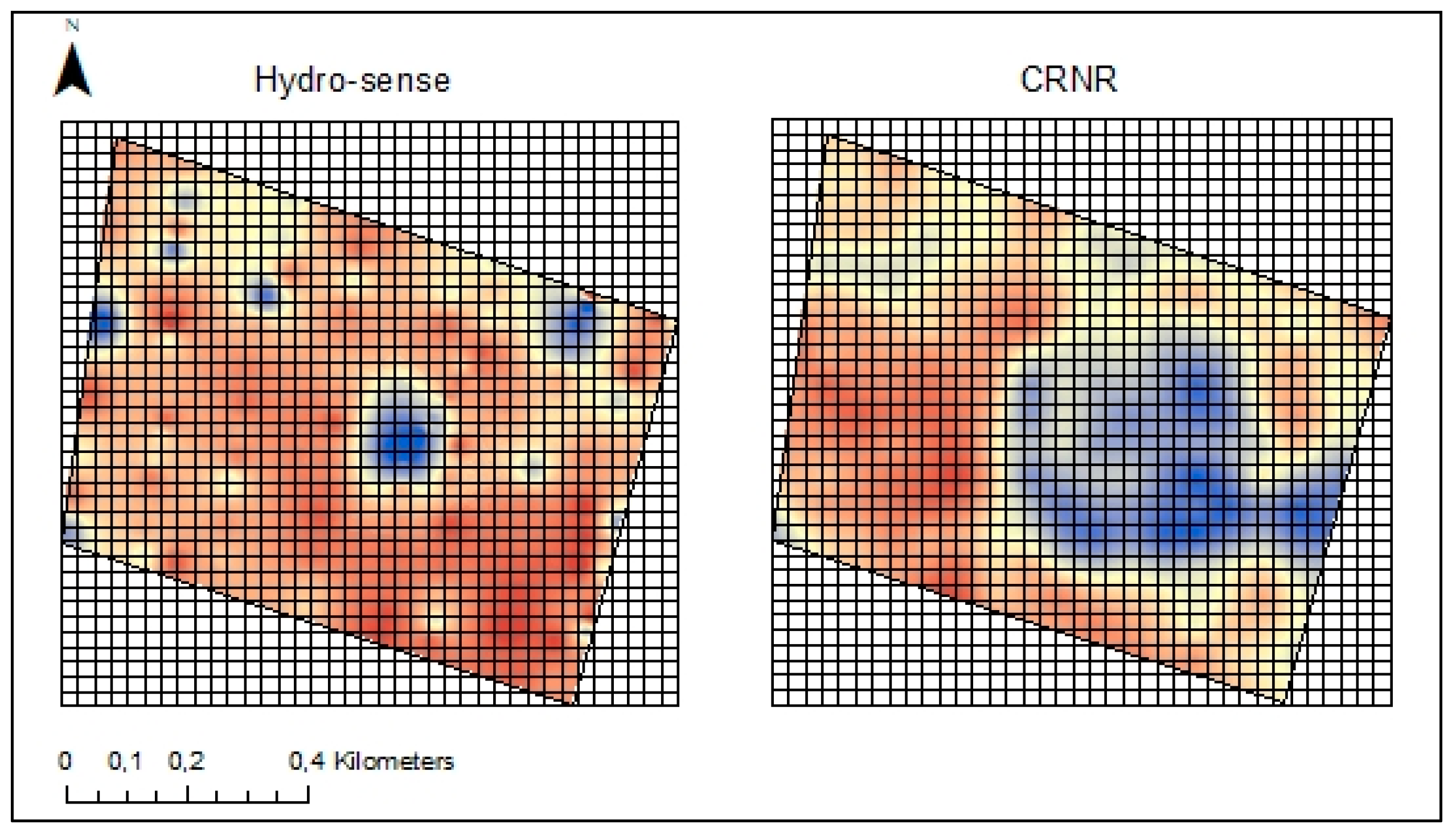
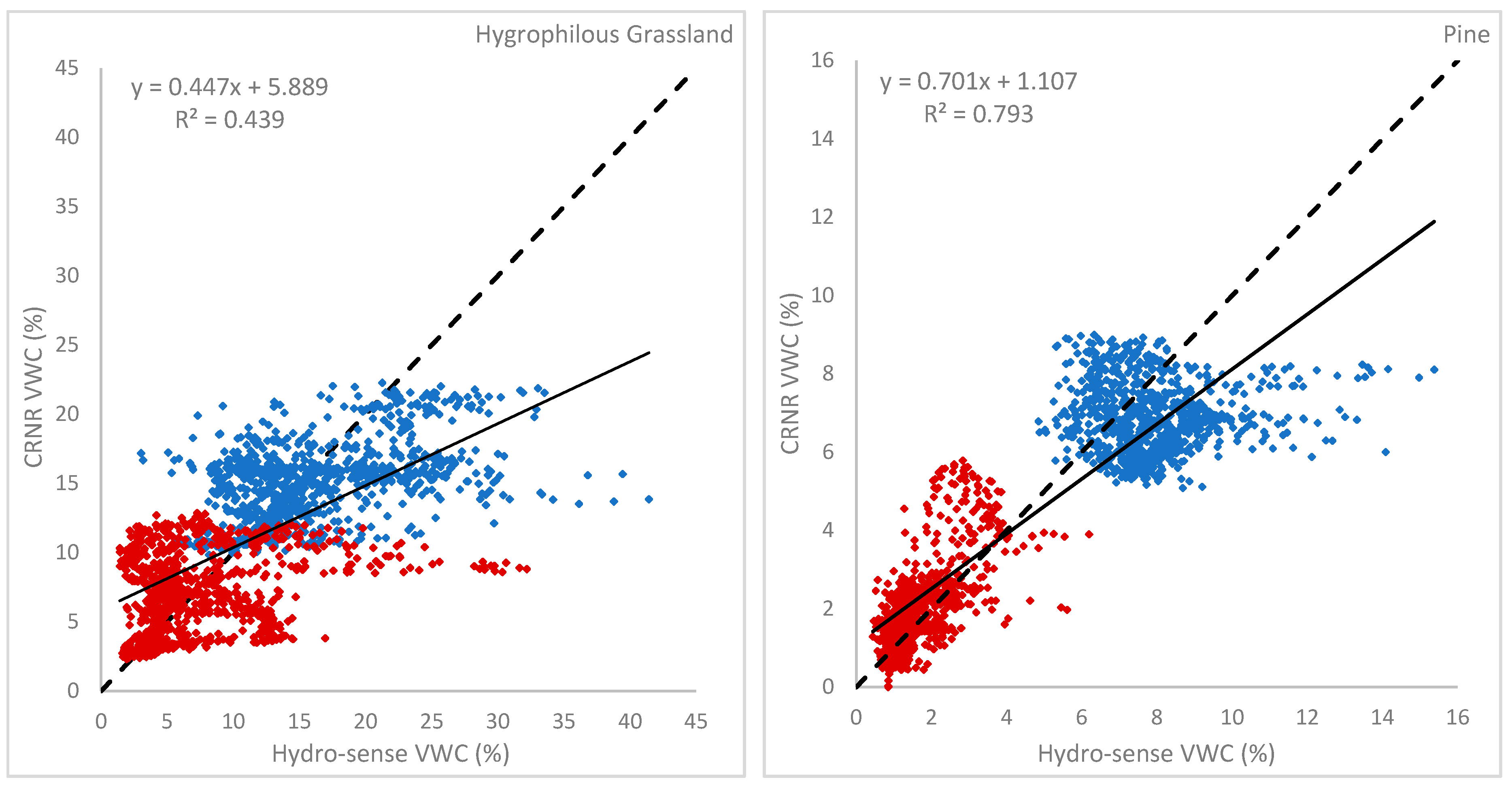
3.2. Cosmic Ray Neutron Rover Validation
4. Conclusions and Recommendations
Supplementary Materials
Author Contributions
Funding
Conflicts of Interest
References
- Zreda, M. Land-surface hydrology with cosmic-ray neutrons: Principles and applications. J. Jpn. Soc. Soil Phys. 2016, 132, 25–30. [Google Scholar]
- Baatz, R.; Bogena, H.R.; Franssen, J.H.; Huisman, J.A.; Montzka, C.; Vereecken, H. An empirical vegetation correction for soil water content quantification using cosmic ray probes. Water Resour. Res. 2015, 51, 2030–2046. [Google Scholar] [CrossRef]
- Ochsner, T.E.; Cosh, M.H.; Cuenca, R.H.; Dorigo, W.A.; Draper, C.S.; Hagimoto, Y.; Kerr, Y.H.; Larson, K.M.; Njoku, E.G.; Small, E.E.; et al. State of the art in large-scale soil moisture monitoring. Soil Sci. Soc. Am. J. 2013, 77, 1888–1919. [Google Scholar] [CrossRef]
- Stocker, B.D.; Zscheischler, J.; Keenan, T.F.; Prentice, I.C.; Seneviratne, S.I.; Peñuelas, J. Drought impacts on terrestrial primary production underestimated by satellite monitoring. Nat. Geosci. 2019. [Google Scholar] [CrossRef]
- McJannet, D.; Hawdon, A.; Baker, B.; Renzullo, L.; Searle, R. Multiscale soil moisture estimates using static and roving cosmic-ray soil moisture sensors. Hydrol. Earth Syst. Sci. 2017, 21, 6049–6067. [Google Scholar] [CrossRef]
- Walker, J.P.; Dumedah, G.; Monerris, A.; Gao, Y.; Rudiger, C.; Wu, X.; Panciera, R.; Merlin, O.; Pipunic, R.; Ryu, D.; et al. High Resolution Soil Moisture Mapping. In Digital Soil Assessments and Beyond, Proceedings of the Fifth Global Workshop on Digital Soil Mapping, Sydney, Australia, 10–13 April 2012; CRC Press: Boca Raton, FL, USA, 2012; pp. 45–51. [Google Scholar]
- Rosolem, R.; Hoar, T.; Arellano, A.; Anderson, J.L.; Shuttleworth, W.J.; Zeng, X.; Franz, T.E. Translating aboveground cosmic-ray neutron intensity to high-frequency soil moisture profiles at sub-kilometer scale. Hydrol. Earth Syst. Sci. 2014, 18, 4363–4379. [Google Scholar] [CrossRef]
- McCabe, M.F.; Rodell, M.; Alsdorf, D.E.; Miralles, D.G.; Uijlenhoet, R.; Wagner, W.; Lucieer, A.; Houborg, R.; Verhoest, N.E.C.; Franz, T.E.; et al. The future of Earth observation in hydrology. Hydrol. Earth Syst. Sci. 2017, 21, 3879–3914. [Google Scholar] [CrossRef]
- Zreda, M.; Shuttleworth, W.J.; Zeng, X.; Zweck, C.; Desilets, D.; Franz, T.; Rosolem, R. COSMOS: The COsmic-ray Soil Moisture Observing System. Hydrol. Earth Syst. Sci. 2012, 16, 4079–4099. [Google Scholar] [CrossRef]
- Franz, T.E.; Zreda, M.; Rosolem, R.; Ferre, T.P.A. Field Validation of a cosmic-ray neutron sensor using a distributed sensor network. Vadose Zone J. 2012, 11. [Google Scholar] [CrossRef]
- Zreda, M.; Desilets, D.; Ferre, T.P.A.; Scott, R.L. Measuring soil moisture content non-invasively at intermediate spatial scale using cosmic-ray neutrons. Geophys. Res. 2008, 35. [Google Scholar] [CrossRef]
- Dong, J.; Ochsner, T.E.; Zreda, M.; Cosh, M.H.; Zou, C.B. Calibration and Validation of the COSMOS Rover for Surface Soil Moisture Measurement. Vadose Zone J. 2014, 13. [Google Scholar] [CrossRef]
- Köhli, M.; Schrön, M.; Zreda, M.; Schmidt, U.; Dietrich, P.; Zacharias, S. Footprint characteristics revised for field-scale soil moisture monitoring with cosmic-ray neutrons. Water Resour. Res. 2015, 10, 5772–5790. [Google Scholar] [CrossRef]
- Desilets, D.; Zreda, M.; Ferre, T.P.A. Nature’s neutron probe: Land surface hydrology at an elusive scale with cosmic rays. Water Resour. Res. 2010, 46, 1–7. [Google Scholar] [CrossRef]
- Chrisman, B.; Zreda, M. Quantifying mesoscale soil moisture with the cosmic-ray rover. Hydrol. Earth Syst. Sci. 2013, 17, 5097–5108. [Google Scholar] [CrossRef]
- Franz, T.E.; Wang, T.; Avery, W.; Finkenbiner, C.; Brocca, L. Combined analysis of soil moisture measurements from roving and fixed cosmic ray neutron probes for multiscale real-time monitoring. Geophys. Res. Lett. 2015, 42, 3389–3396. [Google Scholar] [CrossRef]
- Schrön, M.; Rosolem, R.; Köhli, M.; Piussi, L.; Schroter, I.; Iwema, J.; Kogler, S.; Oswald, S.E.; Wollschlager, U.; Dietrich, P.; et al. The Cosmic-Ray Neutron Rover—Mobile Surveys of Field Soil Moisture and the Influence of Roads. Water Resour. Res. 2018, 54, 6441–6459. [Google Scholar] [CrossRef]
- Fersch, B.; Jagdhuber, T.; Schrön, M.; Volksch, I.; Jager, M. Synergies for soil moisture retrieval across scales from airborne polarimetric SAR, cosmic ray neutron roving, and an in situ sensor network. Water Resour. Res. 2018, 54. [Google Scholar] [CrossRef]
- Finkenbiner, C.E.; Franz, T.E.; Gibson, J.; Heeren, D.M.; Luck, J. Integration of hydrogeophysical datasets and empirical orthogonal functions for improved irrigation water management. Precis. Agric. 2019, 20, 78–100. [Google Scholar] [CrossRef]
- Gibson, J.; Franz, T.E. Spatial prediction of near surface soil water retention functions using hydrogeophysics and empirical orthogonal functions. J. Hydrol. 2018, 561, 372–383. [Google Scholar] [CrossRef]
- Grundling, A.T.; van den Berg, E.C.; Price, J.S. Assessing the distribution of wetlands over wet and dry periods and land-use change on the Maputaland Coastal Plain, north-eastern KwaZulu-Natal, South Africa. S. Afr. J. Geomat. 2013, 2, 120–138. [Google Scholar]
- Zhu, X.; Shao, M.; Zeng, C.; Jia, X.; Huang, L.; Zhang, Y.; Zhu, J. Application of cosmic-ray neutron sensing to monitor soil water content in an alpine meadow ecosystem on the northern Tibetan Plateau. J. Hydrol. 2016, 536, 247–254. [Google Scholar] [CrossRef]
- Shuttleworth, W.J.; Zreda, M.; Zeng, X.; Zweck, C.; Ferre, T.P.A. The COsmic-ray Soil Moisture Observing System (COSMOS): A non-invasive, intermediate scale soil moisture measurement network. British. Hydrol. Soc. 2010, 12, 14551. [Google Scholar]
- Mcjannet, D.; Franz, T.; Hawdon, A.; Boadle, D.; Baker, B.; Almeida, A.; Silberstein, R.; Lambert, T.; Desilets, D. Field testing of the universal calibration function for determination of soil moisture with cosmic-ray neutrons. Water Resour. Res. 2014, 50. [Google Scholar] [CrossRef]
- Franz, T.E.; Zreda, M.; Ferre, T.P.A.; Rosolem, R. An assessment of the effect of horizontal soil moisture heterogeneity on the area-average measurement of cosmic-ray neutrons. Water Resour. Res. 2013, 49, 1–9. [Google Scholar] [CrossRef]
- Schrön, M.; Köhli, M.; Scheiffele, L.; Iwema, J.; Bogena, H.R.; Lv, L.; Martini, E.; Baroni, G.; Rosolem, R.; Weimar, J.; et al. Improving Calibration and Validation of Cosmic-Ray Neutron Sensors in the Light of Spatial Sensitivity—Theory and Evidence. Hydrol. Earth Syst. Sci 2017. [Google Scholar] [CrossRef]
- Desilets, D.; Zreda, M. Footprint diameter for a cosmic-ray soil moisture probe: Theory and Monte Carlo simulations. Water Resour. Res. 2013, 49, 3566–3575. [Google Scholar] [CrossRef]
- Desilets, D. Radius of Influence for a Cosmic-Ray Soil Moisture Probe: Theory and Monte Carlo Simulations; Sandia National Laboratories: Livermore, CA, USA, 2011. [Google Scholar]
- Franz, T.E.; Zreda, M.; Ferre, T.P.A.; Rosolem, R.; Zweck, C.; Stillman, S.; Zeng, X.; Shuttleworth, W.J. Measurement depth of the cosmic ray soil moisture probe affected by hydrogen from various sources. Water Resour. Res. 2012, 48. [Google Scholar] [CrossRef]
- Andreasen, M.; Jensen, K.H.; Desilets, D.; Franz, T.E.; Zreda, M.; Bogena, H.R.; Looms, M.C. Status and Perspectives on the Cosmic-Ray Neutron Method for Soil Moisture Estimation and Other Environmental Science Applications. Vadose Zone J. 2017, 16. [Google Scholar] [CrossRef]
- Montzka, C.; Bogena, H.R.; Zreda, M.; Monerris, A.; Morrison, R.; Muddu, S.; Vereecken, H. Validation of Spaceborne and Modelled Surface Soil Moisture Products with Cosmic-Ray Neutron Probes. Remote Sens. 2017, 9, 103. [Google Scholar] [CrossRef]
- Vather, T.; Everson, C.S.; Mengistu, M.G.; Franz, T.E. Cosmic ray neutrons provide innovative technique for estimating intermediate scale soil moisture. S. Afr. J. Sci. 2018, 114, 79–87. [Google Scholar] [CrossRef]
- Baroni, G.; Oswald, S.E. A scaling approach for the assessment of biomass changes and rainfall interception using Cosmic-Ray neutron sensing. J. Hydrol. 2015, 525, 264–276. [Google Scholar] [CrossRef]
- Rosolem, R.; Shuttleworth, W.J.; Zreda, M.; Franz, T.E.; Zeng, X.; Kurc, S.A. The Effect of Atmospheric Water Vapor on Neutron Count in the Cosmic-Ray Soil Moisture Observing System. J. Hydrometeorol. 2013, 2013, 1659–1671. [Google Scholar] [CrossRef]
- Hawdon, A.; Mcjannet, D.; Wallace, J. Calibration and correction procedures for cosmic-ray neutron soil moisture probes located across Australia. Water Resour. Res. 2014, 50, 5029–5043. [Google Scholar] [CrossRef]
- Avery, W.A.; Finkenbiner, C.; Franz, T.E.; Wang, T.; Nguy-Robertson, A.L.; Suyker, A.; Arkebauer, T.; Munoz-Arriola, F. Incorporation of globally available datasets into the roving cosmic-ray neutron probe method for estimating field-scale soil water content. Hydrol. Earth Syst. Sci. 2016, 20, 3859–3872. [Google Scholar] [CrossRef]
- Babaeian, E.; Sadeghi, M.; Franz, T.E.; Jones, S.; Tuller, M. Mapping soil moisture with the OPtical TRApezoid Model (OPTRAM) based on long-term MODIS observations. Remote Sens. Environ. 2018, 211, 425–440. [Google Scholar] [CrossRef]


| Survey | Hygrophilous Grassland | Pine |
|---|---|---|
| One | 23 November 2016 | 24 November 2016 |
| Two | 15 February 2017 | 17 February 2017 |
| Three | 30 May 2017 | 31 May 2017 |
| Four | 29 January 2018 | 30 January 2018 |
| Hygrophilous Grassland (cpm) | Average Error | Pine (cpm) | Average Error | |
|---|---|---|---|---|
| Survey one | 131.406 | −2.034 | 133.043 | 0.375 |
| Survey two | 135.475 | 2.034 | 132.293 | −0.375 |
| Average | 133.441 | - | 132.668 | - |
| Hygrophilous grassland | ||||
| Survey | Three | Four | ||
| Dataset | Hydro-sense | CRNR | Hydro-sense | CRNR |
| Mean | 7.369 | 7.232 | 16.220 | 15.103 |
| Standard Error | 0.162 | 0.087 | 0.195 | 0.091 |
| Standard Deviation | 5.038 | 2.697 | 6.073 | 2.828 |
| Kurtosis | 4.529 | −1.016 | 0.315 | −0.292 |
| Skewness | 1.873 | 0.081 | 0.804 | 0.338 |
| Range | 30.792 | 10.547 | 38.407 | 12.439 |
| Minimum | 1.407 | 2.303 | 3.020 | 9.825 |
| Maximum | 32.198 | 12.850 | 41.426 | 22.263 |
| Pine | ||||
| Survey | Three | Four | ||
| Dataset | Hydro-sense | CRNR | Hydro-sense | CRNR |
| Mean | 1.713 | 2.069 | 7.905 | 6.888 |
| Standard Error | 0.030 | 0.040 | 0.052 | 0.031 |
| Standard Deviation | 0.882 | 1.167 | 1.510 | 0.891 |
| Kurtosis | 2.444 | 1.060 | 2.932 | −0.654 |
| Skewness | 1.462 | 1.139 | 1.288 | 0.316 |
| Range | 5.750 | 5.788 | 10.529 | 3.912 |
| Minimum | 0.445 | 0.000 | 4.848 | 5.085 |
| Maximum | 6.195 | 5.788 | 15.377 | 8.997 |
| Hygrophilous Grassland | Pine | |||||
|---|---|---|---|---|---|---|
| Performance Metric | RMSE | Bias | ubRMSE | RMSE | Bias | ubRMSE |
| Survey Three | 5.221 | −0.137 | 5.220 | 0.961 | 0.308 | 0.910 |
| Survey Four | 5.514 | −1.118 | 5.400 | 2.032 | −0.880 | 1.832 |
© 2019 by the authors. Licensee MDPI, Basel, Switzerland. This article is an open access article distributed under the terms and conditions of the Creative Commons Attribution (CC BY) license (http://creativecommons.org/licenses/by/4.0/).
Share and Cite
Vather, T.; Everson, C.; Franz, T.E. Calibration and Validation of the Cosmic Ray Neutron Rover for Soil Water Mapping within Two South African Land Classes. Hydrology 2019, 6, 65. https://doi.org/10.3390/hydrology6030065
Vather T, Everson C, Franz TE. Calibration and Validation of the Cosmic Ray Neutron Rover for Soil Water Mapping within Two South African Land Classes. Hydrology. 2019; 6(3):65. https://doi.org/10.3390/hydrology6030065
Chicago/Turabian StyleVather, Thigesh, Colin Everson, and Trenton E. Franz. 2019. "Calibration and Validation of the Cosmic Ray Neutron Rover for Soil Water Mapping within Two South African Land Classes" Hydrology 6, no. 3: 65. https://doi.org/10.3390/hydrology6030065
APA StyleVather, T., Everson, C., & Franz, T. E. (2019). Calibration and Validation of the Cosmic Ray Neutron Rover for Soil Water Mapping within Two South African Land Classes. Hydrology, 6(3), 65. https://doi.org/10.3390/hydrology6030065