Application of HEC-HMS Model for Flow Simulation in the Lake Tana Basin: The Case of Gilgel Abay Catchment, Upper Blue Nile Basin, Ethiopia

Abstract
:1. Introduction
2. Methodology
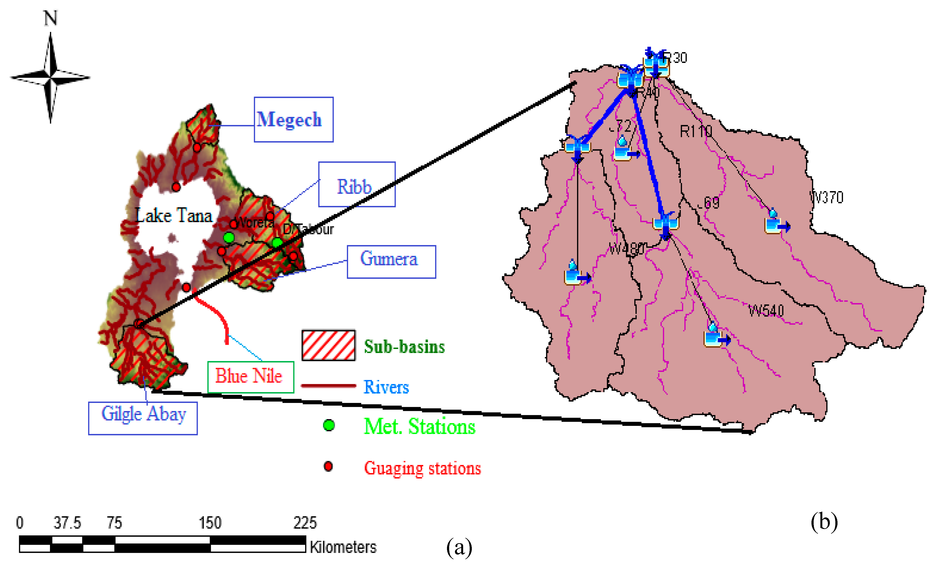
2.1. Study Area Description
2.2. Data
2.3. Models
2.3.1. HEC-HMS Model
2.3.2. HEC-GeoHMS Model
2.4. Model Calibration and Validation
3. Results and Discussion
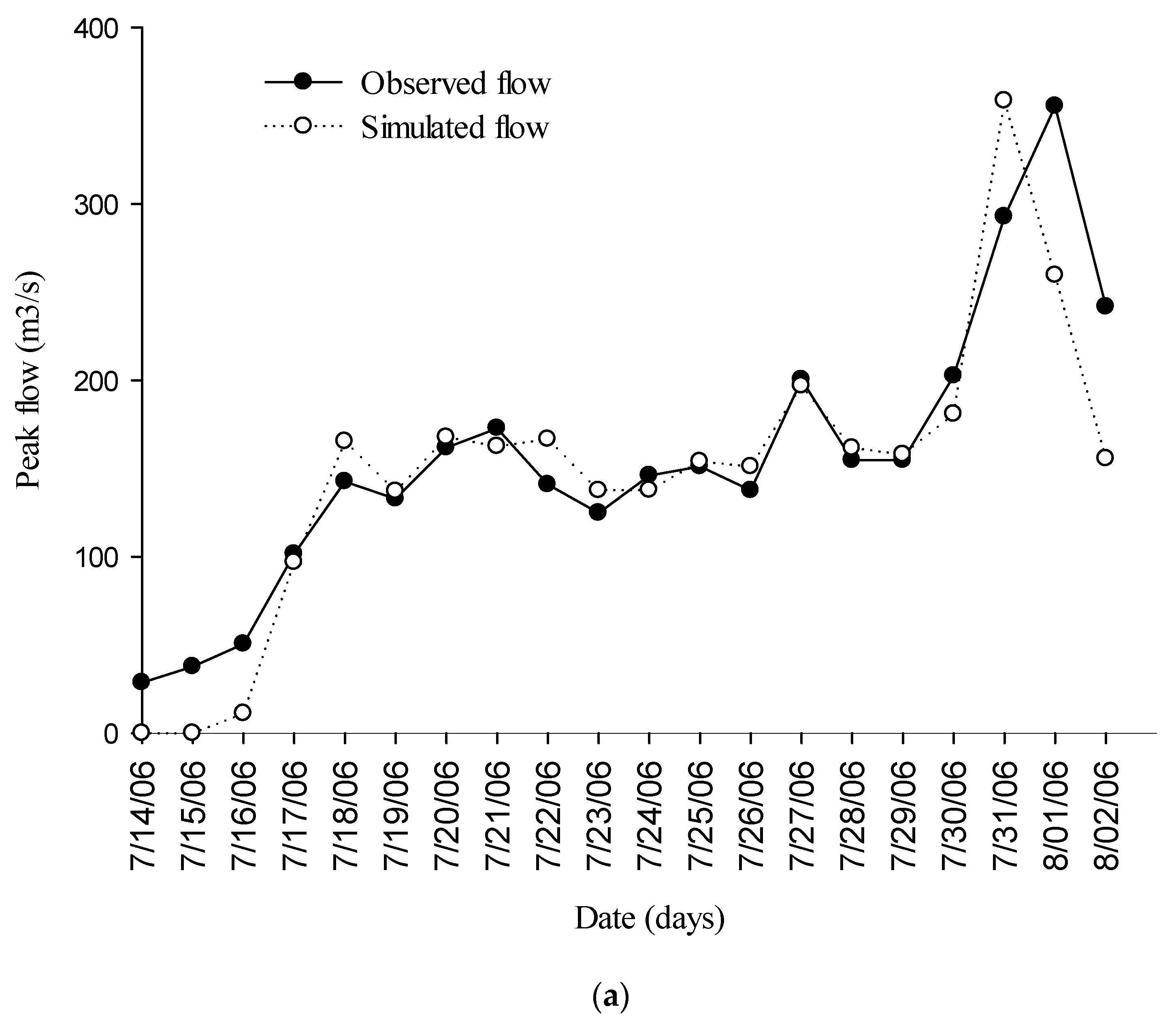
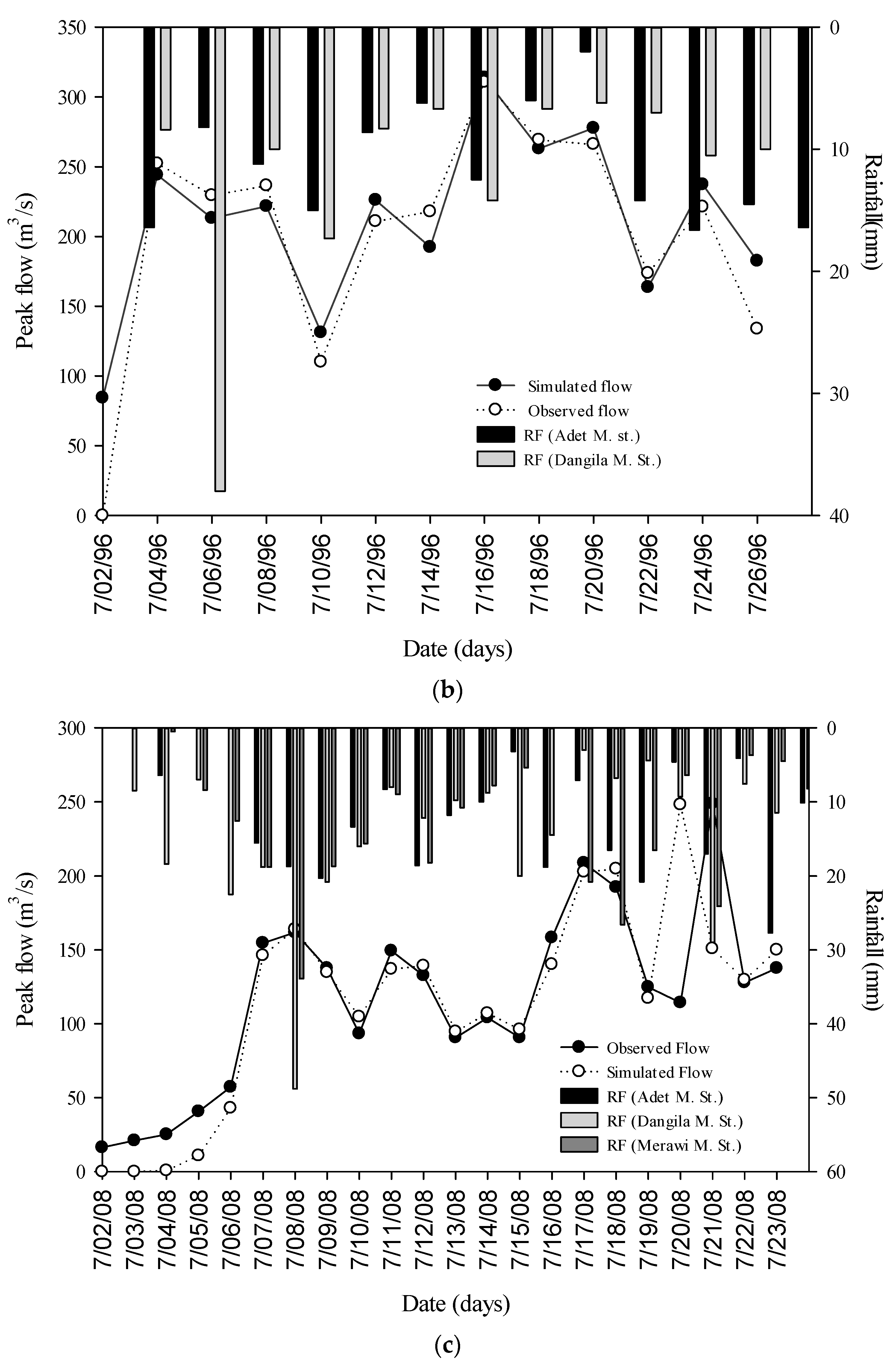
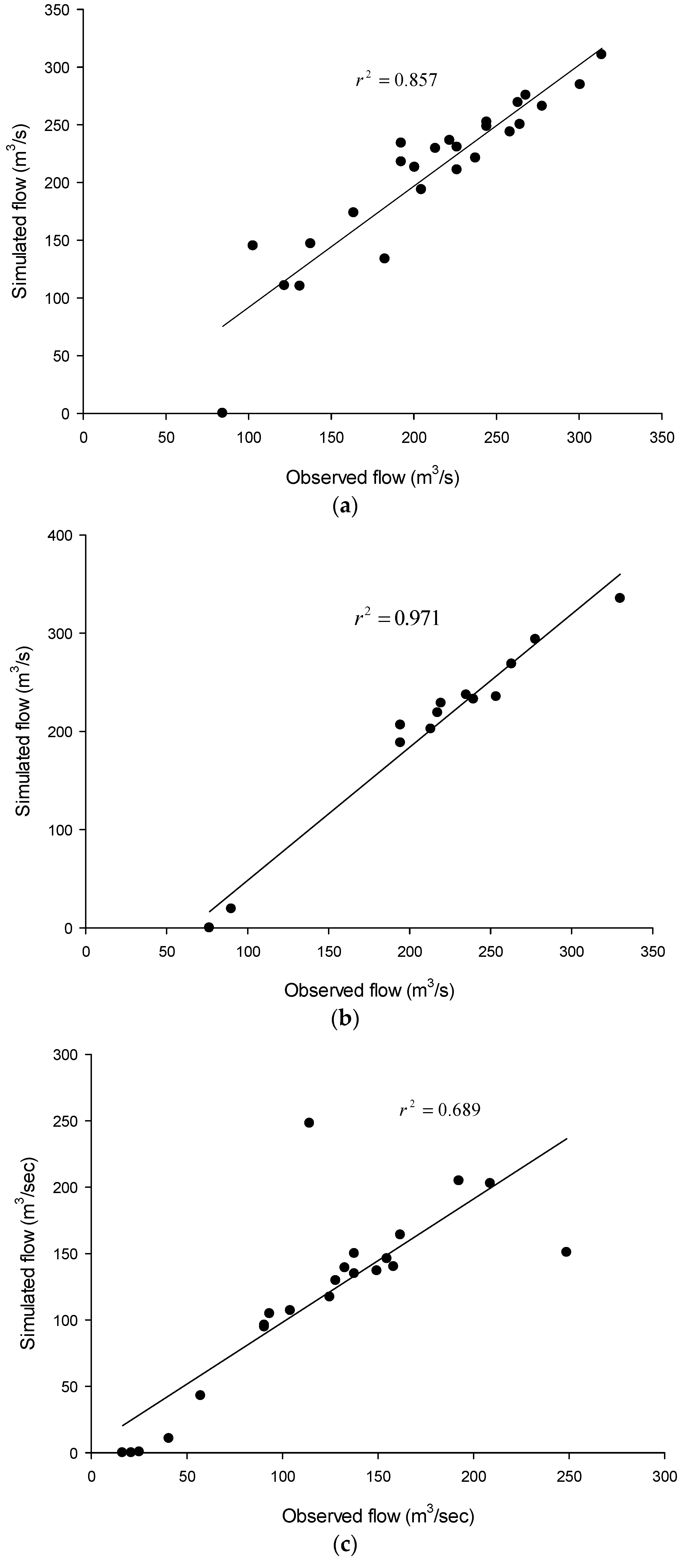
3.1. Calibration
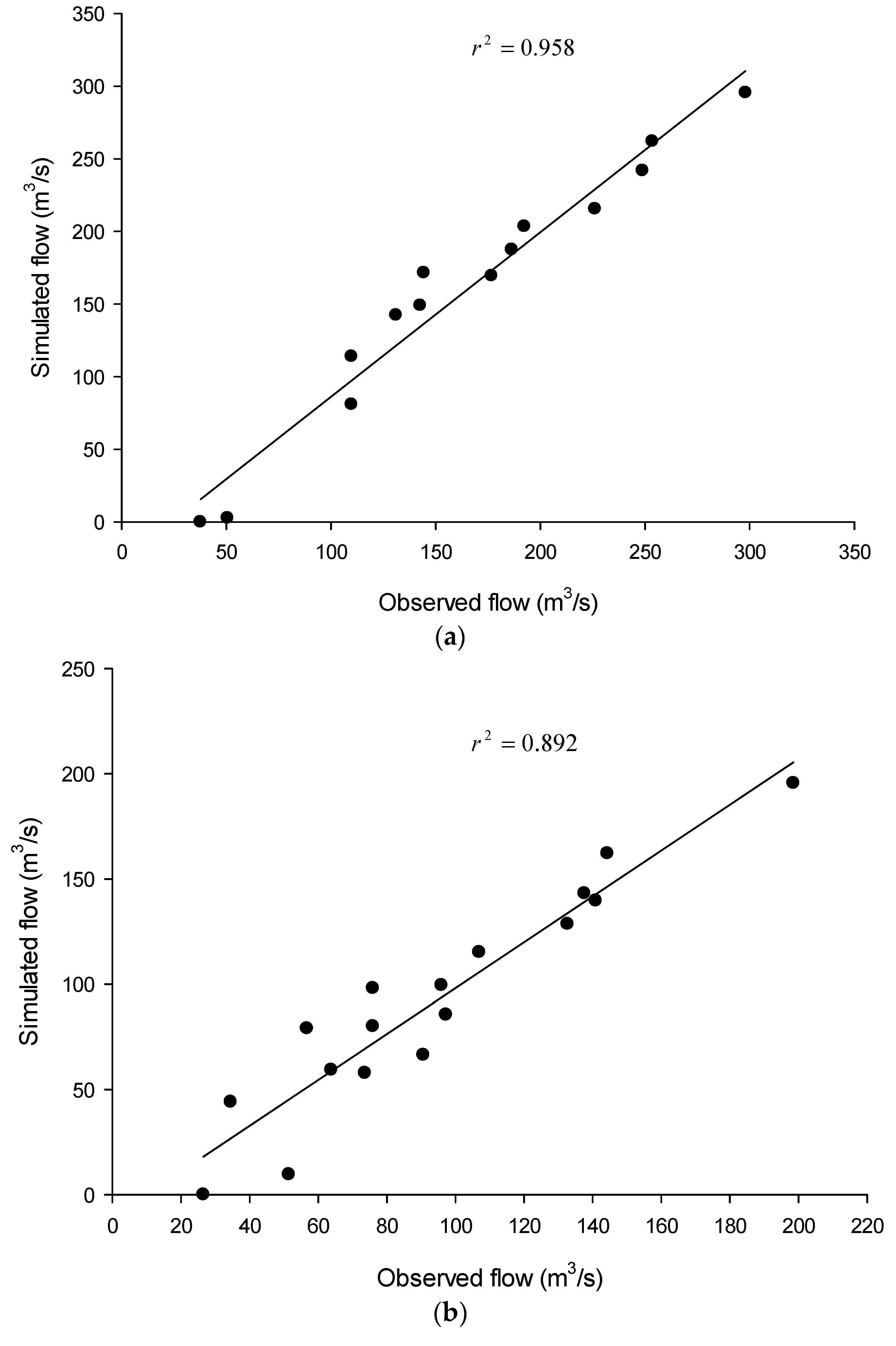
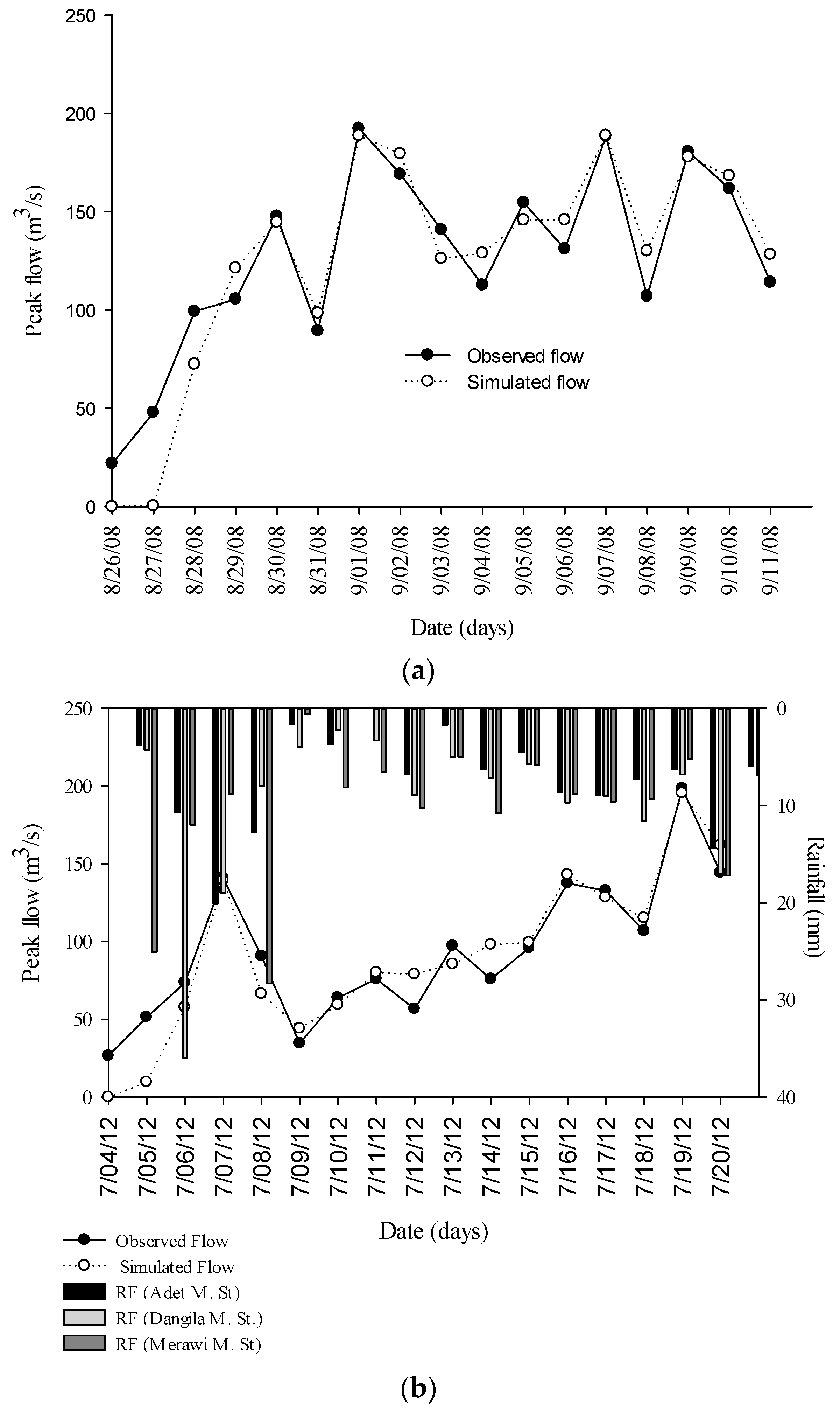
3.2. Validation
4. Conclusions
Author Contributions
Funding
Acknowledgments
Conflicts of Interest
References
- Zhang, W.W.; Fu, B.J.; Meng, Q.H.; Zhang, Q.J.; Zhang, Y.H. Effects of land-use pattern change on rainfall-runoff and runoff-sediment relations: A case study in Zichang watershed of the Loess Plateau of China. J. Environ. Sci. 2004, 16, 436–442. [Google Scholar]
- Beven, K.J. Rainfall-Runoff Modelling: The Primer; John Wiley & Sons: Chichester, UK; Wiley-Blackwell: Hoboken, NJ, USA, 2012. [Google Scholar]
- Jia, Y.; Zhao, H.; Niu, C.; Jiang, Y.; Gan, H.; Xing, Z.; Zhao, Z.A. WebGIS-based system for rainfall-runoff prediction and real-time water resources assessment for Beijing. Comput. Geosci. 2009, 35, 1517–1528. [Google Scholar] [CrossRef]
- Cunderlik, M.J. Hydrologic Model Selection Fort the CFCAS Project: Assessment of Water Resources Risk and Vulnerability to Changing Climatic Conditions; Department of Civil and Environmental Engineering, The University of Western Ontario: London, ON, Canada, 2003. [Google Scholar]
- Bedient, P.B.; Holder, A.; Benavides, J.A.; Vieux, B.E. Radar-based flood warning system applied to Tropical Storm Allison. J. Hydrol. Eng. 2003, 8, 308–318. [Google Scholar] [CrossRef]
- Shi, H.; Li, T.; Liu, R.; Chen, J.; Li, J.; Zhang, A.; Wang, G. A service-oriented architecture for ensemble flood forecast from numerical weather prediction. J. Hydrol. 2015, 527, 933–942. [Google Scholar] [CrossRef]
- Halwatura, D.; Najim, M. Application of the HEC-HMS model for runoff simulation in a tropical catchment. Environ. Modell. Softw. 2013, 46, 155–162. [Google Scholar] [CrossRef]
- US Army Corps of Engineers. Hydrologic Modeling System, HEC-HMS. Quick Start Guide; US Army Corps of Engineers, Institute for Water Resources, Hydrologic Engineering Center: Davis, CA, USA, 2015.
- Chu, X.; Steinman, A. Event and continuous hydrologic modeling with HEC-HMS. J. Irrig. Drain. E-Asce. 2009, 135, 119–124. [Google Scholar] [CrossRef]
- Zelelew, D.; Melesse, A. Applicability of a Spatially Semi-Distributed Hydrological Model for Watershed Scale Runoff Estimation in Northwest Ethiopia. Water 2018, 10, 923. [Google Scholar] [CrossRef]
- Al-Abed, N.; Abdulla, F.; Khyarah, A.A. GIS-hydrological models for managing water resources in the Zarqa River basin. Environ. Geol. 2005, 47, 405–411. [Google Scholar] [CrossRef]
- Radmanesh, F.; Hemat, J.P.; Behnia, A.; Khond, A.; Mohamad, B.A. Calibration and assessment of HEC-HMS model in Roodzard watershed. In Proceedings of the 17th international conference of river engineering, Ahvaz, Iran, 2006. [Google Scholar]
- Sardoii, E.R.; Rostami, N.; Sigaroudi, S.K.; Taheri, S. Calibration of loss estimation methods in HEC-HMS for simulation of surface runoff (Case Study: Amirkabir Dam Watershed, Iran). Adv. Environ. Biol. 2012, 6, 343–348. [Google Scholar]
- Fallah, S. Simulation of maximum peak discharge in river tributaries using HEC-HMS model (Case study: Moha mmadabad watershed, Golestan province). Master’s Thesis, University of Gorgan, Gorgan, Iran, 2001. [Google Scholar]
- Yusop, Z.; Chan, C.; Katimon, A. Runoff characteristics and application of HEC-HMS for modelling stormflow hydrograph in an oil palm catchment. Water Sci. Technol. 2007, 56, 41–48. [Google Scholar] [CrossRef] [PubMed]
- Yener, M.K.; Sorman, A.U.; Sorman, A.A.; Sensoy, A.; Gezgin, T. Modeling studies with HEC-HMS and runoff scenarios in Yuvacik Basin, Turkiye. Int. Congr. River Basin Manag. 2007, 4, 621–634. [Google Scholar]
- Yilma, H.M.; Moges, S.A. Application of semi-distributed conceptual hydrological model for flow forecasting on upland catchments of Blue Nile River Basin, a case study of Gilgel Abbay catchment. Catchment Lake Res. 2007, 6, 1–200. [Google Scholar]
- Merrey, D.J.; Gebreselassie, T. Promoting Improved Rainwater and Land Management in the Blue Nile (Abay) Basin of Ethiopia: Annexes. ILRI: Nairobi, Kenya; Department for International Development: London, UK, 2011.
- Bitew, M.; Gebremichael, M. Assessment of satellite rainfall products for streamflow simulation in medium watersheds of the Ethiopian highlands. Hydrol. Earth Syst. Sci. 2011, 15, 1147–1155. [Google Scholar] [CrossRef]
- Azam, M.; San Kim, H.; Maeng, S.J. Development of flood alert application in Mushim stream watershed Korea. Int. J. Disast. Risk Re. 2017, 21, 11–26. [Google Scholar] [CrossRef]
- Feldman, A. Hydrologic Modeling System HEC-HMS Technical Reference Manua; US Army Corps of Engineers. Hydrologic Engineering Center: Davis, CA, USA, 2000.
- US Army Corps of Engineers. Hydrologic Modeling System (HEC-HMS) Application Guide Version 3.1.0; Institute for Water Resources: Davis, CA, USA, 2008.
- Banitt, A. Simulating a century of hydrographs e Mark Twain reservoir. In Proceedings of the 2nd Joint Federal Interagency Conference, Las Vegas, NV, USA, 27 June–1 Julyy 2010. [Google Scholar]
- Bajwa, H.; Tim, U. Toward immersive virtual environments for GIS-based Floodplain modeling and Visualization. In Proceedings of the 22nd ESRI User Conference, San Diego, CA, USA, 8–12 Julyy 2002. [Google Scholar]
- Kamali, B.; Mousavi, S. Automatic calibration of HEC-HMS model using multi-objective fuzzy optimal models. CEIJ 2014, 47, 1–12. [Google Scholar]
- Jin, H.; Liang, R.; Wang, Y.; Tumula, P. Flood-runoff in semi-arid and sub-humid regions, a case study: A simulation of jianghe watershed in northern China. Water 2015, 7, 5155–5172. [Google Scholar] [CrossRef]
- Environmental and Water Resources Instit. Curve Number Hydrology: State of the Practice; Hawkins, R.H., Ward, T.J., Woodward, D.E., Van Mullem, J.A., Eds.; American Society of Civil Engineers: Reston, VA, USA, 2009. [Google Scholar]
- Mockus, V. Estimation of Total (and Peak Rates of) Surface Runoff for Individual Storms. Exhibit A in Appendix B, Interim Survey Report, Grand (Neosho) River Watershed; USDA: Washington, DC, USA, 1949.
- Lastra, J.; Fernández, E.; Díez-Herrero, A.; Marquínez, J. Flood hazard delineation combining geomorphological and hydrological methods: An example in the Northern Iberian Peninsula. Nat. Hazards 2008, 45, 277–293. [Google Scholar] [CrossRef]
- Heshmatpoor, A. Identification runoff source area in tropical watershed. In Proceedings of the Postgraduate Qolloquium Semester, Kuala Lumpur, Malaysia, 26–29 October 2009. [Google Scholar]
- Kirpich, Z. Time of concentration of small agricultural watersheds. Civ. Eng. 1940, 10, 362. [Google Scholar]
- McCarthy, G.T. The unit hydrograph and flood routing. In Proceedings of the Conference of North Atlantic Division, Washington, WA, USA, 1938. [Google Scholar]
- Shaw, E.M. Hydrology in Practice; T.J. International Ltd.: Cornwall, UK, 1994. [Google Scholar]
- Tewolde, M.H.; Smithers, J. Flood routing in ungauged catchments using Muskingum methods. Water SA 2006, 32, 379–388. [Google Scholar] [CrossRef]
- Birkhead, A.; James, C. Muskingum river routing with dynamic bank storage. J. Hydrol. 2002, 264, 113–132. [Google Scholar] [CrossRef]
- Merwade, V. Watershed and Stream Network Delineation Using ArcHydro Tools; School of Civil Engineering, Purdue University: West Lafayette, IN, USA, 2012; pp. 1–7. [Google Scholar]
- Hamby, D. A review of techniques for parameter sensitivity analysis of environmental models. Environ. Monit. Assess. 1994, 32, 135–154. [Google Scholar] [CrossRef] [PubMed]
- Majidi, A.; Shahedi, K. Simulation of rainfall-runoff process using Green-Ampt method and HEC-HMS model (Case study: Abnama Watershed, Iran). J. Hydraul. Eng. 2012, 1, 5–9. [Google Scholar]
- Najim, M.M.M.; Babelb, M.S.; Loofb, R. AGNPS Model Assessment for a Mixed Forested Watershed in Thailand. ScienceAsia 2006, 32, 53–61. [Google Scholar]
- Nash, J.E.; Sutcliffe, J.V. River flow forecasting through conceptual models part I—A discussion of principles. J. Hydrol. 1970, 10, 282–290. [Google Scholar] [CrossRef]
- Gupta, H.V.; Kling, H.; Yilmaz, K.K.; Martinez, G.F. Decomposition of the mean squared error and NSE performance criteria: Implications for improving hydrological modelling. J. Hydrol. 2009, 377, 80–91. [Google Scholar] [CrossRef]
- Neter, J.; Wasserman, W.; Kutner, M.H. Applied Statistical Models; Richard D. Irwin, Inc.: Burr Ridge, IL, USA, 1990. [Google Scholar]
- Reed, S.; Koren, V.; Smith, M.; Zhang, Z.; Moreda, F.; Seo, D.J.; Participants, D.M.I.P. Overall distributed model intercomparison project results. J. Hydrol. 2004, 298, 27–60. [Google Scholar] [CrossRef]
- Sabzevari, T.; Ardakanian, R.; Shamsaee, A.; Talebi, A. Estimation of flood hydrograph in no statistical watersheds using HEC-HMS model and GIS (Case study: Kasilian watershed). J. Water Eng. 2009, 4, 1–11. [Google Scholar]
- Cheng, C.-T.; Ou, C.; Chau, K. Combining a fuzzy optimal model with a genetic algorithm to solve multi-objective rainfall–runoff model calibration. J. Hydrol. 2002, 268, 72–86. [Google Scholar] [CrossRef]
- Gupta, H.V.; Sorooshian, S.; Yapo, P.O. Status of automatic calibration for hydrologic models: Comparison with multilevel expert calibration. J. Hydrol. Eng. 1999, 4, 135–143. [Google Scholar] [CrossRef]
- Zou, K.H.; Tuncali, K.; Silverman, S.G. Correlation and simple linear regression. Radiology 2003, 227, 617–628. [Google Scholar] [CrossRef] [PubMed]
- Moriasi, D.N.; Arnold, J.G.; Van Liew, M.W.; Bingner, R.L.; Harmel, R.D.; Veith, T.L. Model evaluation guidelines for systematic quantification of accuracy in watershed simulations. Trans. ASABE 2007, 50, 885–900. [Google Scholar] [CrossRef]
- Gharib, M.; Motamedvaziri, B.; Ghermezcheshmeh, B.; Ahmadi, H. Evaluation Of Modclark Model For Simulating Rainfall-Runoff In Tangrah Watershed, Iran. Appl. Ecol. Env. Res. 2018, 16, 1053–1068. [Google Scholar] [CrossRef]
- Zelelew, D.G. Spatial mapping and testing the applicability of the curve number method for ungauged catchments in Northern Ethiopia. J. Soil Water Conserv. 2017, 5, 293–301. [Google Scholar] [CrossRef]
- Hawkins, R.H. Asymptotic determination of runoff curve numbers from data. J. Irrig. Drain. Eng. 1993, 119, 334–345. [Google Scholar] [CrossRef]
- Jin, X.; Xu, C.Y.; Zhang, Q.; Chen, Y.D. Regionalization study of a conceptual hydrological model in Dongjiang basin, south China. Quat. Int. 2009, 208, 129–137. [Google Scholar] [CrossRef]


| Events | Start Date | Start Time | End Date | End Time | Remark |
|---|---|---|---|---|---|
| Event 1 | 02 Julyy 1996 | 00:00 | 26 July 1996 | 00:00 | Calibration |
| Event 2 | 16 Aug1996 | 00:00 | 31 August 1996 | 00:00 | Calibration |
| Event 3 | 14 July 2006 | 00:00 | 02 August 2006 | 00:00 | Calibration |
| Event 4 | 05 August 2006 | 00:00 | 17 August 2006 | 00:00 | Calibration |
| Event 5 | 01 September 2006 | 00:00 | 19 August 2006 | 00:00 | Calibration |
| Event 6 | 02 July 2008 | 00:00 | 23 July 2006 | 00:00 | Calibration |
| Event 7 | 02 August 2008 | 00:00 | 15 August 2008 | 00:00 | Validation |
| Event 8 | 26 August 2008 | 00:00 | 11 September 2008 | 00:00 | Validation |
| Event 9 | 04 July 2012 | 00:00 | 20 July 2012 | 00:00 | Validation |
| Event 10 | 08 August 2012 | 00:00 | 23 August 2012 | 00:00 | Validation |
| Sub-Catchment Code | Area(km2) | Perimeter (km) | Slope (%) | CN * | Lag (h) |
|---|---|---|---|---|---|
| W340 | 232.59 | 124.800 | 17.73 | 85.00 | 3.26 |
| W370 | 480.07 | 189.240 | 23.30 | 84.67 | 4.44 |
| W480 | 356.49 | 155.560 | 18.6 | 84.47 | 3.88 |
| W540 | 540.22 | 175.520 | 24.97 | 84.87 | 2.94 |
| Events | Peak Discharge (m3/s) | Total Volume (mm) | NSE | R2 | ||||||
|---|---|---|---|---|---|---|---|---|---|---|
| Simulated | Observed | REP | Simulated | Observed | REV | |||||
| BOP | AOP | BOP | AOP | |||||||
| Event 1 | 341.8 | 310.6 | 313.8 | 1.02 | 206.56 | 276.02 | 275.83 | −0.07 | 0.812 | 0.857 |
| Event 2 | 365.2 | 286.7 | 277.7 | −3.24 | 112.01 | 146.00 | 154.03 | 5.21 | 0.707 | 0.856 |
| Event 3 | 505.8 | 358.6 | 355.5 | −0.87 | 242.31 | 154.67 | 160.85 | 3.84 | 0.769 | 0.803 |
| Event 4 | 511.9 | 335.2 | 330.1 | −1.54 | 154.31 | 137.3 | 142.64 | 3.74 | 0.794 | 0.971 |
| Event 5 | 427.2 | 227.1 | 217.3 | −4.51 | 138.93 | 160.3 | 158.49 | −1.14 | 0.788 | 0.876 |
| Event 6 | 429.2 | 248.1 | 248.8 | 0.28 | 197.08 | 131.34 | 134.79 | 2.56 | 0.603 | 0.689 |
| Mean | 430.2 | 294.4 | 290.5 | 1.91 | 175.2 | 167.6 | 171.1 | 2.76 | 0.746 | 0.842 |
| S.No. | Methods | Parameter | Values | |
|---|---|---|---|---|
| Calculated | Optimized | |||
| 1 | Loss rate parameter | CN scale factor | 1.1892 | 0.8977 |
| Ia scale factor | 0.9815 | 1.0527 | ||
| Impervious area (%) | 0.0 | 0.0 | ||
| 2 | Runoff Transform | Lag time | 217.738 | 217.738 |
| 3 | Routing Method constants | K | 0.5 | 0.5 |
| X | 0.1 | 0.1 | ||
| Parameters | Ia Scale Factor | CN Scale Factor | Tlag | K | X |
|---|---|---|---|---|---|
| Events | |||||
| Event 1 | 0.83672 | 1.1721 | 217.738 | 0.5 | 0.1 |
| Event 2 | 0.97046 | 0.8813 | 217.738 | 0.5 | 0.1 |
| Event 3 | 1.515 | 0.91532 | 217.738 | 0.5 | 0.1 |
| Event 4 | 1.015 | 0.81121 | 217.738 | 0.5 | 0.1 |
| Event 5 | 0.98892 | 1.0074 | 217.738 | 0.5 | 0.1 |
| Event 6 | 0.9898 | 0.59913 | 217.738 | 0.5 | 0.1 |
| Mean | 1.0527 | 0.8977 | 217.738 | 0.5 | 0.1 |
| Events | Peak Discharge (m3/s) | Total Volume (mm) | NSE | R2 | ||||
|---|---|---|---|---|---|---|---|---|
| Simulated | Observed | REP | Simulated | Observed | REV | |||
| Event 7 | 295.4 | 298.0 | 0.87 | 115.99 | 119.05 | 2.57 | 0.922 | 0.958 |
| Event 8 | 188.9 | 192.4 | 1.82 | 111.77 | 112.54 | 0.678 | 0.848 | 0.908 |
| Event 9 | 195.5 | 198.5 | 1.51 | 79.56 | 81.47 | 2.34 | 0.847 | 0.892 |
| Event 10 | 242.1 | 246.4 | 1.75 | 121.31 | 126.26 | 3.92 | 0.919 | 0.943 |
| Mean | 230.5 | 233..8 | 1.49 | 107.16 | 109.83 | 2.38 | 0.884 | 0.925 |
© 2019 by the authors. Licensee MDPI, Basel, Switzerland. This article is an open access article distributed under the terms and conditions of the Creative Commons Attribution (CC BY) license (http://creativecommons.org/licenses/by/4.0/).
Share and Cite
Tassew, B.G.; Belete, M.A.; Miegel, K. Application of HEC-HMS Model for Flow Simulation in the Lake Tana Basin: The Case of Gilgel Abay Catchment, Upper Blue Nile Basin, Ethiopia. Hydrology 2019, 6, 21. https://doi.org/10.3390/hydrology6010021
Tassew BG, Belete MA, Miegel K. Application of HEC-HMS Model for Flow Simulation in the Lake Tana Basin: The Case of Gilgel Abay Catchment, Upper Blue Nile Basin, Ethiopia. Hydrology. 2019; 6(1):21. https://doi.org/10.3390/hydrology6010021
Chicago/Turabian StyleTassew, Bitew G., Mulugeta A. Belete, and K. Miegel. 2019. "Application of HEC-HMS Model for Flow Simulation in the Lake Tana Basin: The Case of Gilgel Abay Catchment, Upper Blue Nile Basin, Ethiopia" Hydrology 6, no. 1: 21. https://doi.org/10.3390/hydrology6010021
APA StyleTassew, B. G., Belete, M. A., & Miegel, K. (2019). Application of HEC-HMS Model for Flow Simulation in the Lake Tana Basin: The Case of Gilgel Abay Catchment, Upper Blue Nile Basin, Ethiopia. Hydrology, 6(1), 21. https://doi.org/10.3390/hydrology6010021