Spatial Heterogeneity of Snow Density and Its Influence on Snow Water Equivalence Estimates in a Large Mountainous Basin

Abstract

Accurate representation of the spatial distribution of snow water equivalent (SWE) in mountainous basins is critical for furthering the understanding of snow as a water resource, especially in the Western United States. To estimate the spatial distribution and total volume of SWE over mountainous basins, previous work has either assumed uniform snow density or used simple approaches to estimate density. This study uses over 1000 direct measurements of SWE and snow depth (from which density was calculated) in sampling areas that were physiographically proportional to a large (207 km²) mountainous basin in southwest Montana. Using these data, modeled spatial distributions of density and depth were developed and combined to obtain estimates of total basin SWE. Six estimates of SWE were obtained using varying combinations of the distributed depth and density models and were compared to the average of three different models that utilized direct measurements of SWE. Models utilizing direct SWE measurements varied by approximately 1% around their mean, while SWE estimates derived from combined depth and density models varied by over 14% around the same mean. This study highlights the need to carefully consider the spatial variability of density when estimating SWE based on snow depth in these environments.

1. Introduction and Background

Water accumulated and stored in the winter snowpack of mountainous regions constitutes a critical source of annual streamflow for much of the Western United States, providing approximately 75% of annual discharge [1]. Improved understanding of how snow water equivalent (SWE) is spatially distributed in mountainous terrain can assist hydrologic models to provide better estimates of total basin SWE and forecasts of the timing, magnitude and seasonal volume of snowmelt runoff. Such information is valuable for a number of applications, such as agricultural planning, reservoir management and flood forecasting, among others.

The spatial distribution of SWE can be highly variable in mountainous terrain [2], where its understanding is most critical for quantifying snow as a water resource. Associations between physiographic characteristics of a basin (e.g., elevation, radiation, vegetation, aspect, slope angle) and SWE at a given point have been used to estimate the spatial distribution of SWE in mountainous terrain using various field sampling and statistical methods, e.g., [2,3,4,5,6,7,8,9]. However, there are many substantial challenges to such studies in both field data collection and modeling methods to provide the most accurate representations of the spatial distribution and total volume of SWE in a basin. In particular, when SWE is not directly measured, but rather estimated using snow depth and either a fixed density value or one that is varied based on a single parameter (e.g., elevation). Therefore, when using this approach, one of the major challenges is the characterization of the spatial distribution of snow density, which is a critical component to calculating SWE. This is important because while proportionally, the differences in snow density may be conservative when compared to depth due to its limited range of potential values, when used to calculate SWE, a relatively small change in density can have a substantial impact on an estimate of total basin SWE [10].

Due to the highly dynamic nature of snow characteristics, particularly near the time of peak accumulation, it is optimal for the field data collection to occur as quickly as possible to minimize the bias from temporal changes in the snow. Because of the time-consuming nature of obtaining density samples, previous field-based studies have sampled more intensively for depth than for density (or SWE directly), e.g., [2,4,5,6,8]. This approach must be carefully balanced with an assurance that the density data collected are representative of the time and place of interest. Previous research has stated that snow depth varies more than snow density in alpine areas, so the major source of variation in SWE is variation in snow depth, especially during the melt season [3,11]. However, few studies have quantified these effects and how they vary near the time of peak accumulation. This challenge has also been noted by Adams [12], who suggests that while variability in density lessens throughout the melt season, before, the primary onset of melt density exhibits considerable variability. This can be further exacerbated in high relief mountain areas where the timing of melt and, therefore, inhomogeneity in density at a fixed point in time can be considerable.

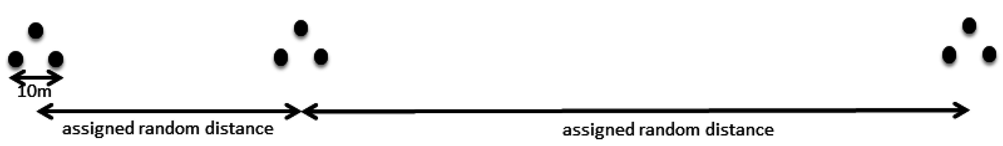
The spatial arrangement of samples, both with respect to the greater basin and to each other, in a given study can also have a substantial influence on the resulting analysis and modeling [13]. It is possible that variability in snow density that exists in the field may not be captured statistically if sampling is not specifically designed to do so. Studies have attempted to capture the effects of physiography on the spatial distribution of density [4,8] by choosing sample locations that qualitatively represent the different elevations and aspects of the given watershed. This methodology may not account for unique combinations (and interactions) of multiple physiographic parameters that may be associated with density. Research has noted scale breaks in snow depth within which sampling should take place [14], but no similar research has specifically been applied to density.

The spatial distribution of the snow density component of SWE models has been parameterized in several ways in previous research. In some cases, a uniform spatial distribution of the average of measured densities [6,8] is used due to the poor results of models correlating density to independent variables. Other research has found significant correlations between density and basin physiography [4,5], but with only a small number of density samples (n = 10 or less). Snow depth has also been assumed to provide a direct corollary to SWE, making the assumption of uniform (although not specified) density throughout a basin [7]. Many of these findings, often using small sample sizes, have not quantified the effect varying parameterizations of depth and density may have on estimates of SWE. Lopez-Moreno et al. [9] used three different model types to predict the spatial distribution of snow density in three small (1–2 km²) plots in the Spanish Pyrenees, but these models were deemed largely inadequate due to the marked variability in correlations between density and depth, as well as other terrain characteristics examined.

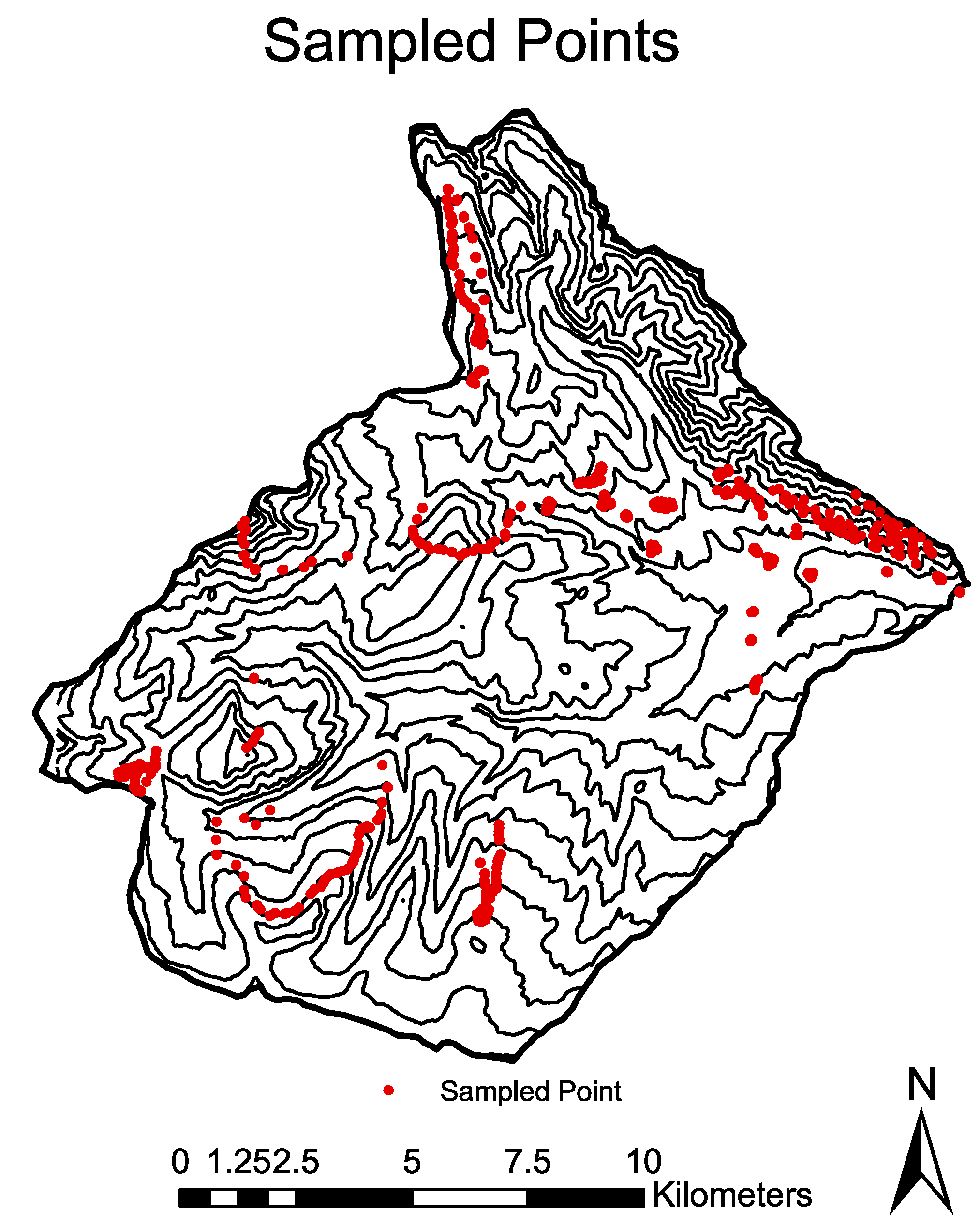
This paper presents a comprehensive field study aimed at modeling the effect of the spatial variability of snow density in estimating total basin SWE for a complex mountainous watershed. A novel sampling strategy was used to collect a very large number of samples (>1000) of SWE and snow depth (allowing for calculation of density) throughout a 207-km² mountainous basin. Three models of the spatial distribution of snow density were developed and combined with two models of the spatial distribution on snow depth to obtain estimates of total basin SWE. An analysis of the effect of varying parameterizations of snow depth and density on estimates of the total volume of SWE stored in a basin is provided. This study highlights that snow density can be highly variable near the time of peak accumulation, especially in a high relief basin. This indicates the importance of adequate sampling and modeling of snow density if separate depth and density models are to be used for SWE estimations, as estimates of total basin SWE can vary widely depending on the models used.

2. Study Area

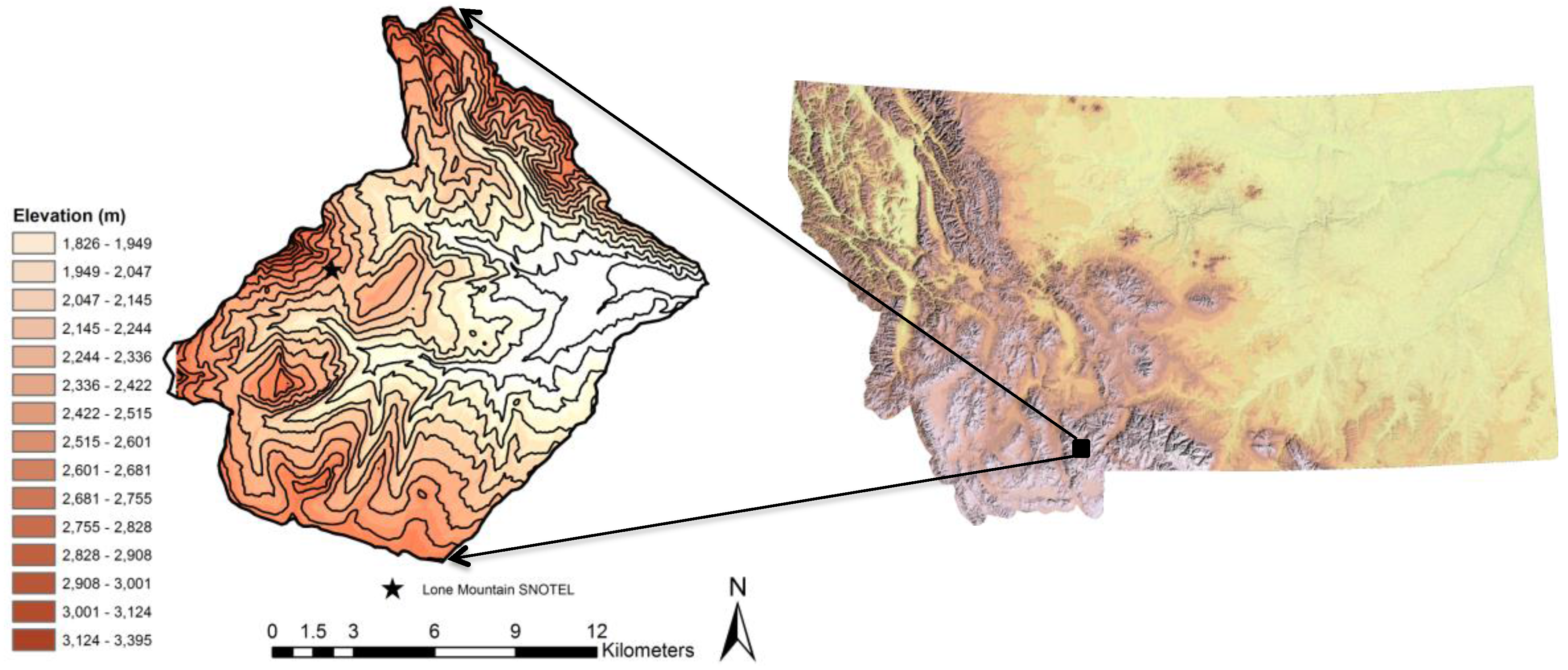
This study was conducted in the West Fork of the Gallatin River Basin (West Fork Basin) in southwest Montana, approximately 45°16′N, 111°26′W (Figure 1). Elevations in the basin range from 1825 m at the confluence of the West Fork of the Gallatin with the Gallatin River to 3405 m at the top of Lone Peak (1580 m of total vertical relief), covering an area of 207 km². The West Fork Basin is physiographically diverse, ranging from low elevation grass and sagebrush cover, to mid-elevation conifer forests, to high elevation steep rocky alpine terrain. Approximately 52% of the basin contains conifer forests, with the land cover in the remaining areas consisting primarily of grass and sagebrush in the lower elevations and rocky alpine terrain at the higher elevations. The basin is partially developed, containing a small community (Big Sky, MT, USA) and ski resorts on Lone Peak and Pioneer mountains in the western portion of the basin.

The only automated SWE data for the basin is provided by the Lone Mountain SNOwpack TELemetry (SNOTEL) site, located in a small meadow in the west-central portion of the basin at an elevation of 2706 m. As of 1 April 2012 (the time of field sampling), the Lone Mountain SNOTEL site was reporting 104% of median SWE based on a 21-year record (1991–2012), at 434 mm.

Figure 1. Location map showing the state of Montana, USA, with an inset of the West Fork of the Gallatin River Basin in southwest Montana; 100-m contour interval. The star shows the location of the Lone Mountain SNOTEL site.

Figure 1. Location map showing the state of Montana, USA, with an inset of the West Fork of the Gallatin River Basin in southwest Montana; 100-m contour interval. The star shows the location of the Lone Mountain SNOTEL site.

3. Methods

3.1. Sampling Strategy

Due to the relatively large size of the West Fork Basin, sampling throughout its entirety was not a practical option. To resolve this challenge, smaller portions of the basin, termed “sampling areas”, were defined that were physiographically proportional to the whole [15]. These definitions were based on unique combinations of defined ranges of elevation, potential incoming solar radiation and forest cover, as they are well accepted to be associated with SWE [2] (Table 1). These unique combinations will be referred to as physiographic strata.

To define the physiographic strata, grids of elevation and potential incoming solar radiation were classified into five and four distinct categories, respectively, while the land cover grid was classified as either forested or un-forested. The solar radiation metric used was potential net accumulated 1 December 2011–1 April 2012 in watt-hours per square meter (Wh/m²), calculated using ESRI ArcGIS 10.0. Physiographic strata were defined through the use of map algebra applied to reclassified raster datasets of the aforementioned parameters through raster addition. Each parameter was classified on a different order of magnitude, so when added together, they provided unique identifiers of which unique combination of parameters comprises each strata, as seen in Table 1.

Table 1. Reclassification parameters for defining sampling strata.

Parameter	Value(s)	Classified Value
Elevation (m)	1820–2139	1000
	2140–2453	2000
	2454–2767	3000
	2768–3081	4000
	3082–3395	5000
Potential radiation (Wh/m2)	63,919–176,897	100
(1 December–1 April)	176,898–228,251	200
	228,252–279,604	300
	279,605–391,299	400
Forest cover	Unforested	0
	Forested	10

Table 1. Reclassification parameters for defining sampling strata.

Parameter	Value(s)	Classified Value
Elevation (m)	1820–2139	1000
	2140–2453	2000
	2454–2767	3000
	2768–3081	4000
	3082–3395	5000
Potential radiation (Wh/m2)	63,919–176,897	100
(1 December–1 April)	176,898–228,251	200
	228,252–279,604	300
	279,605–391,299	400
Forest cover	Unforested	0
	Forested	10

As an example, if a given strata had an identifier of 1410, that strata is in the lowest elevation band (1000), receives the highest levels of solar radiation (0400) and is forested (0010). Through this process, 36 unique strata were defined to identify and justify which portions of the basin were to be sampled. Sampling areas were chosen based on accessibility and the physiographic representativeness of the basin as a whole. Physiographic representativeness was determined by comparing the proportion of each strata within the defined sampling areas to the proportion of the strata in the basin as a whole.

3.2. Data Collection

The field data collection campaign took place from 30 March to 3 April 2012 near the time of peak SWE accumulation, as recorded at the Lone Mountain SNOTEL site. SWE and snow depth measurements were acquired using Federal SWE Samplers, a process where a core of the snowpack is acquired and weighed on a spring scale, which reports inches of water content in the sample [16]. These data and every sample location were recorded using Global Positioning System (GPS) receivers. The positional accuracy of these points was sub-meter after post-processing and was adequate given that the scale of the analysis rasters was 30 m. Sets of three samples were taken as 10-meter equilateral triangles to minimize bias due to anisotropy [17]. These sets of three samples were acquired at randomly-assigned distances that varied (as best estimated by sampling teams) from 30 m to 400 m between them (Figure 2) as teams of two travelled throughout the defined sampling areas. Sampling teams travelled throughout the defined sampling areas acquiring SWE and snow depth measurements at the pre-assigned random distances along their path. The range of spatial scales at which sampling occurred was chosen based on the findings of Watson et al. [17] and the results of pilot studies to ensure sampling teams could adhere to the sampling plan while travelling throughout the entirety of a sampling area. By sampling at random distances over spatial scales of 10 m and 400 m, variations in snow depth were captured within multiple frequency intervals (as observed by Trujillo et al. [14]). This allowed for the sampling of interactions between SWE depth and the surrounding physiography over both small and large spatial extents. Additionally, given that any point at a certain distance away from a random starting point (i.e., previously-sampled location) is equally representative as any other point the same distance away, the effect of random sampling was achieved through the systematic sampling of a random field [17,18].

Figure 2. Example of the field data collection plan.

Figure 2. Example of the field data collection plan.

The randomization of the distances at which samples are taken allows for a more robust statistical analysis [19]. Much of this sampling theory was also influenced by the importance of the scale triplet in spatial sampling, where the spacing, extent and support of field samples collected are used to define the spatial dimensions of a field study. In this context, the spacing is the distance between samples, the extent is the size of the domain sampled and the support is the averaging area of one sample [13,20]. In total, 1043 direct measurements of SWE and snow depth (and therefore density) were measured and recorded, the locations of which are shown in Figure 3. All sample points were acquired within the defined sampling areas, which constituted approximately 25% of the total basin area. Samples also well represented the distribution of physiographic strata in the basin [15]. A small subset of samples (<5%) was acquired within ski area boundaries in areas minimally impacted by resort operations, as recommended by ski patrol, with the goal of best mimicking natural conditions.

Figure 3. The locations of all sampled points in the basin; 100-m contour interval.

Figure 3. The locations of all sampled points in the basin; 100-m contour interval.

3.3. Data Analysis

All GPS data collected in the field using Trimble GeoXH receivers were converted into a single shapefile with SWE and snow depth values attached to each point feature as an attribute (from which density was calculated). The GPS data were post-processed to obtain sub-meter accuracy for the majority of points collected. Physiographic attributes of the point where a sample was collected were then added as attributes of the point feature. These included elevation, potential incoming solar radiation under clear sky conditions (total accumulated from 1 December–1 April as Wh/m²), land cover (as forested or not), slope angle, aspect and degree of curvature (second derivative) of the land surface. All parameters, with the exception of land cover, were derived from a USGS 30-m DEM [8]. While no direct indices related to wind redistribution or wind exposure were included, as observed by Golding [21] and Woo et al. [22], the degree of curvature could be correlated to wind, with snow being removed from convex areas and re-deposited in concave areas.

Samples that were assumed to be inaccurate due to measurement or recording error were identified and removed from the dataset by calculating the density for each sample and applying a 95% prediction interval to a simple linear regression of elevation on snow density. Observations that occurred outside the prediction interval were assumed to have error in either measurement or recording and were removed from the dataset, representing 26 data points. The dataset used for analysis consisted of 1017 measurements of SWE, snow depth, snow density and the selected physiographic attributes of each point, chosen based on the findings of Clark et al. [2].

3.4. Models for Quantifying Density, Depth and SWE

Multiple linear regression (MLR) [23] and binary regression tree analysis [24] were used to model the spatial distribution of snow density using correlations to basin physiography. MLR is a method for quantifying correlations between multiple physiographic parameters (e.g., elevation and potential incoming radiation) and snow density, providing a means of estimating densities based on the basin characteristics at any given point in the basin using linear relationships. Binary regression tree analysis is a method that recursively splits the dataset based on physiographic parameters to minimize the residual mean square error (RMSE) at each node in the tree. The optimal tree size for the data (number of terminal nodes) is determined by defining a complexity parameter at which model performance no longer substantially improves by including more nodes, based on a 10-fold cross-validated error.

These two types of models were chosen because of their different approaches to regression-based modeling. This allows for a comparison of two sound statistical techniques that produce results in notably different formats. The regression tree provides a discrete number of modeled densities, while the MLR model produces a continuum of unique modeled values. The results of these statistical models were applied to the gridded datasets of the significant physiographic parameters to estimate their respective spatial distributions of snow density.

To model the spatial distribution of SWE and obtain estimates of total basin SWE, the spatial distribution of snow depth was modeled using mixed effects multiple regression (MEMR) [25] and binary regression tree analysis. The snow depth data collected in the field did not fully comply with all of the assumptions of multiple linear regression (namely constant variance of the residuals [23]). Because of this, an MEMR model was chosen for snow depth, because it provides a way to analyze those data that do not require a data transformation, where information about important interactions of the explanatory variables may be blurred or lost [25]. In this case, a fixed variance MEMR model structure was used because it accounts for the non-constant variance in the residuals of depth as elevation increases, which an MLR model is not able to do. Similar to the density models, the binary regression tree was also chosen, as it provides a comparison to a notably different type of model output to the MEMR model, which estimates a continuous distribution of values. Six unique combinations of depth and density models were developed to model the spatial distribution of SWE and to estimate total basin SWE. Estimates of total basin SWE derived from these models were compared to the average of three models that utilized direct measurements of SWE using MEMR, binary regression tree analysis and conditional inference (CI) tree analysis. CI tree analysis is a form of recursive partitioning analysis that uses different splitting and stopping criteria than binary regression tree analysis and was chosen as a way to compare the results of two different tree-based analysis methods. The size of a tree is determined by a defined significance level required for a split to occur, a minimum number of observations for a split and a minimum number of observations required for a final node (in this study; 95%, 60% and 30%, respectively), so cross-validation and pruning are not necessary for determining the final tree size [26].

4. Results

4.1. Field Observations

A wide range of SWE, depth and density values was observed during data collection. Generally, the lowest SWE and snow depths and the highest density values were found in the low elevation meadows of the basin and particularly on southerly aspects. Many low elevation areas of the basin were entirely snow free at the time of sampling, most commonly on steep south-facing aspects, but also in other isolated areas throughout the lower elevation portions of the basin. High elevation areas held the most SWE and deepest snow; while the influence of radiation was still evident, it appeared to have less influence at high elevation than in lower portions of the basin. The lowest densities were observed in the higher elevations on northerly aspects. Summary statistics of the field data are shown in Table 2.

Table 2. Summary of observed SWE and snow density data.

Data Type	Minimum	Mean	Maximum	Standard Deviation	n
SWE (mm)	0	246	965	206	1017
Density (kg/m3)	190	349	500	61	1017
Depth (mm)	0	735	2740	620	1017

Table 2. Summary of observed SWE and snow density data.

Data Type	Minimum	Mean	Maximum	Standard Deviation	n
SWE (mm)	0	246	965	206	1017
Density (kg/m3)	190	349	500	61	1017
Depth (mm)	0	735	2740	620	1017

4.2. Results of Multiple Linear Regression Modeling for Snow Density

Initially, simple linear regression (SLR) [23] analysis was performed, testing all available physiographic parameters to determine which had a significant correlation to snow density. Elevation, radiation, slope angle and snow depth all had statistically significant correlations to snow density (Table 3). Elevation had the strongest correlation, explaining 27% of the observed variance. Snow depth also showed a strong correlation, explaining 18% of observed variance. Potential incoming solar radiation on its own explained 13% of observed variance, while that of slope angle was minimal.

Table 3. Summary of the results of the simple linear regression (SLR) of physiographic parameters on snow density.

Model Structure	R2	p-Value
density~elevation	0.27	<2.2 × 10−16
density~radiation	0.13	<2.2 × 10−16
density~snow depth	0.18	<2.2 × 10−16
density~slope angle	0.047	3.89 × 10−10

Table 3. Summary of the results of the simple linear regression (SLR) of physiographic parameters on snow density.

Model Structure	R2	p-Value
density~elevation	0.27	<2.2 × 10−16
density~radiation	0.13	<2.2 × 10−16
density~snow depth	0.18	<2.2 × 10−16
density~slope angle	0.047	3.89 × 10−10

Using the results of the SLR analysis, a stepwise MLR analysis was performed to determine which combinations of parameters best estimate the spatial distribution of density. The model structure utilizing elevation and radiation as predictors provided the best fit for the data, explaining 39% of observed variance in density (Table 4). Using snow depth and radiation, the fit improved over just using snow depth, but was still only slightly better than the SLR of density as a function of elevation alone.

Table 4. Results of multiple linear regression (MLR) models for snow density.

Model Structure	R2	p-Value
density ~ elevation + radiation	0.39	<2.2 × 10−16
density ~ snow depth + radiation	0.28	<2.2 × 10−16

Table 4. Results of multiple linear regression (MLR) models for snow density.

Model Structure	R2	p-Value
density ~ elevation + radiation	0.39	<2.2 × 10−16
density ~ snow depth + radiation	0.28	<2.2 × 10−16

A model utilizing elevation and snow depth together was not used due to their high level of correlation (r² = 0.73). The MLR model that best describes the data is as follows:

Snow density (kg/m³) = 479.5 + −0.1104*elevation (m) + 0.0004878*radiation (WH/m²)

(1)

This model structure estimated a range of snow densities from 184 to 406 kg/m³. The lowest modeled densities are at the highest elevations on slopes that receive the least radiation, while the highest densities are at low elevation on slopes receiving high levels of radiation. The spatial distribution of snow density (Figure 4) was modeled by applying the above formula to raster datasets of elevation and radiation using raster algebra.

Figure 4. The spatial distribution of snow density using a multiple linear regression model. The range of modeled values is 184–406 kg/m³; 100-m contour interval.

Figure 4. The spatial distribution of snow density using a multiple linear regression model. The range of modeled values is 184–406 kg/m³; 100-m contour interval.

Figure 5. Distribution of residuals between measured densities and modeled densities from the multiple linear regression model.

Figure 5. Distribution of residuals between measured densities and modeled densities from the multiple linear regression model.

The continuous distribution of density values estimated using the MLR model can be seen in Figure 4 through the smooth gradient of shades (representing densities) driven by the varying continuums of elevation and incoming solar radiation. This continuous distribution of predicted densities can also be seen in the residual plot in Figure 5. Residuals for this model were normally distributed and slightly negatively skewed, underestimating measured densities by 29 kg/m³ on average and with a mean absolute error (MAE) of 48 kg/m³.

4.3. Results of Regression Tree Modeling for Snow Density

The optimal regression tree for modeling density contained nine terminal nodes and utilized elevation and radiation to model the spatial distribution of snow density throughout the basin (Figure 6). The optimal tree size for this model was determined by pruning the tree back to the value of the complexity parameter at which additional nodes no longer reduced the 10-fold cross-validated error. This method provided a more restricted range of estimated densities (270–366 kg/m³) and a different spatial distribution (Figure 7) than the MLR model. The tree model displayed a slightly improved R² value over MLR, explaining 41% of observed variance in the data.

Figure 6. Binary regression tree utilizing nine terminal nodes to estimate the spatial distribution of snow density.

Figure 6. Binary regression tree utilizing nine terminal nodes to estimate the spatial distribution of snow density.

The discrete nature of modeled density values resulting from the regression tree analysis can be seen in Figure 7 through the very distinct changes in shade, representing changes in density. The abrupt changes that are driven by a split in elevation may not provide the most realistic model of how a change would occur in nature. However, these types of changes do occur over short distances resulting from changes in incoming solar radiation, which are modeled well with the regression tree. This can be seen throughout the basin in Figure 7 with a sharp contrast being commonly modeled between south-facing and north-facing slopes. Another major difference between this and the MLR is that this model estimates a substantial increase in density in the highest elevation range. This could possibly be a result of sampling wind compacted snow in the alpine portions of the basin, but it is anomalous compared to the other trends observed in this analysis. This is a potential weakness of this model, as these conditions are likely not representative of all areas in the highest elevations of the basin. A regression tree model utilizing snow depth in addition to elevation and radiation was also developed and tested. While this model did contain two splits based on depth, it was not chosen for the final analysis due to non-significant improvement over the chosen model and to allow for the comparison between the MLR and regression tree models utilizing the same input parameters.

Residual analysis of the regression tree model also shows residuals being normally distributed with a slightly negative skew (Figure 8). On average, this model under-estimated measured density values by 30 kg/m³, similar to the MLR model, and with a slightly smaller MAE of 46 kg/m³. While the residuals from this model are relatively normally distributed, the residual plots in Figure 5 and Figure 8 also display the contrast between the continuous nature of estimated values from MLR versus the discrete nature of values estimated with the regression tree.

Figure 7. Modeled spatial distribution of snow density using a nine-node regression tree. The range of modeled values is 270–366 kg/m³; 100-m contour interval.

Figure 7. Modeled spatial distribution of snow density using a nine-node regression tree. The range of modeled values is 270–366 kg/m³; 100-m contour interval.

Figure 8. Distribution of residuals between measured densities and modeled densities from the regression tree model.

Figure 8. Distribution of residuals between measured densities and modeled densities from the regression tree model.

4.4. Snow Depth Models

Two spatially-distributed models of snow depth were developed to combine with the density models for the purpose of estimating total basin SWE. The MEMR model utilized elevation, potential incoming solar radiation and forest cover as variables to model a continuous range of snow depth values throughout the basin. The MEMR snow depth model had an MAE of 212 mm, and the model structure is shown below:

Snow depth = −2888 + 1.79*elevation (m) + −0.00233*radiation (WH/m²) + −13.2*land cover (with 10 = forested and 0 = unforested)

(2)

The optimal binary regression tree model was pruned to five terminal nodes based the complexity parameter at which there was no substantial improvement to the 10-fold cross-validated error. Splits were made primarily on elevation, with one split being made on radiation, as the forest cover parameter was not found to provide significant improvement to the model. This model structure had an MAE of 284 mm and is shown below in Figure 9. The modeled spatial distribution of snow depth resulting from these models is shown in Figure 10.

Figure 9. Five terminal node regression tree describing snow depth.

Figure 9. Five terminal node regression tree describing snow depth.

Figure 10. Spatially-distributed snow depth models; the mixed effects multiple regression (MEMR) model on the left and the five-node binary regression tree model on the right.

Figure 10. Spatially-distributed snow depth models; the mixed effects multiple regression (MEMR) model on the left and the five-node binary regression tree model on the right.

4.5. SWE Models from Direct Measurement

Three model structures were developed to estimate SWE utilizing direct field measurements (MEMR, seven-node regression tree and 16-node CI tree). The different methods produced substantially different spatial distributions and ranges of SWE values, but all estimated similar values of total basin SWE, to within approximately 1% of their average (Table 5). MEMR analysis yielded the widest range of modeled values (859 mm) and that most similar to the range of measured values (965 mm). The binary regression tree and conditional inference tree models provided similar ranges of values, 501 mm and 486 mm, respectively. The CI tree provided the lowest MAE at 75 mm, followed by the spatial average of models, MEMR and regression tree models at 82, 87 and 101 mm, respectively.

Table 5. Summary of modeled SWE values from all model structures.

Model	Modeled Total Basin SWE (m3)	Range of Modeled SWE Values (mm)	Mean Absolute Error (mm)	Number of Unique Modeled SWE Values
MEMR	59,792,000	0–859	87	all unique
CI tree	60,935,000	0–486	75	16
Regression tree	61,195,000	43–545	101	7
Average of others	60,641,000	15–618	82	all unique

Table 5. Summary of modeled SWE values from all model structures.

Model	Modeled Total Basin SWE (m3)	Range of Modeled SWE Values (mm)	Mean Absolute Error (mm)	Number of Unique Modeled SWE Values
MEMR	59,792,000	0–859	87	all unique
CI tree	60,935,000	0–486	75	16
Regression tree	61,195,000	43–545	101	7
Average of others	60,641,000	15–618	82	all unique

In addition to differences in the modeled ranges of SWE values and MAE values, the manner in which SWE was distributed throughout the basin (Figure 11) also varied amongst the models. The MEMR model provided the smoothest distribution of values throughout the elevation range. This is in contrast to the regression tree, which modeled no SWE values between 162 and 359 mm, a range of values that contains the mean and median for all measured and modeled values [15]. The CI tree produced a more continuous distribution of modeled values than the regression tree.

Figure 11. Spatially-distributed SWE models resulting from direct SWE measurements.

Figure 11. Spatially-distributed SWE models resulting from direct SWE measurements.

4.6. The Effect of Varying Density and Depth Models on Estimates of Total Basin SWE

Estimates of total basin SWE were acquired by combining two spatially-distributed models of snow depth with the two spatially-distributed snow density models, as well as a spatially-uniform model representing the average of measured densities (349 kg/m³ with an MAE of 52 kg/m³) to obtain estimates of total basin SWE. These estimates of total basin SWE were then compared to the average of total basin SWE as calculated by the three models (MLR, MEMR and regression tree) that utilized direct SWE measurements (60,641,000 m³), shown in Table 6. Total basin SWE estimates derived from models utilizing direct SWE measurements only varied within approximately 1% of their average; these models will be referred to as the control models and their average as the control value. The SWE models resulting from the combined depth and density models varied substantially, by 14.1% around the control value. MAE values for all of the combined models were higher than those resulting from direct measurement, with the exception of the binary regression tree model. The MAE values were also within a relatively small range of each other, but because this metric is expressed as an absolute value it does not capture the over-estimation or under-estimation bias of a given model, which can be gathered from the resulting total basin SWE estimate.

Table 6. The effect of varying depth and density parameterizations on estimates of total basin SWE. Comparisons are being made to the mean volume estimated by the three models utilizing direct measurements of SWE (60,641,000 m³).

Depth Model	Density Model	Modeled Total Basin SWE (m3)	% Difference from Control Value	Mean Absolute Error (mm)
MEMR	MLR	55,973,813	−8.3	92
MEMR	Regression tree	56,728,045	−6.9	91
MEMR	Spatially uniform	59,409,463	−2.1	89
Regression tree	MLR	61,088,312	+0.7	88
Regression tree	Regression tree	61,574,372	+1.5	91
Regression tree	Spatially uniform	64,398,753	+5.8	92

Table 6. The effect of varying depth and density parameterizations on estimates of total basin SWE. Comparisons are being made to the mean volume estimated by the three models utilizing direct measurements of SWE (60,641,000 m³).

Depth Model	Density Model	Modeled Total Basin SWE (m3)	% Difference from Control Value	Mean Absolute Error (mm)
MEMR	MLR	55,973,813	−8.3	92
MEMR	Regression tree	56,728,045	−6.9	91
MEMR	Spatially uniform	59,409,463	−2.1	89
Regression tree	MLR	61,088,312	+0.7	88
Regression tree	Regression tree	61,574,372	+1.5	91
Regression tree	Spatially uniform	64,398,753	+5.8	92

All SWE models that used the MEMR snow depth model produced smaller estimates of total basin SWE than the SWE models utilizing the regression tree snow depth model. SWE estimates resulting from the MEMR depth model were all below the average of the control models, and those resulting from the regression tree depth model were all above the control value. Variation in total basin SWE estimates within the two depth models used also followed a consistent pattern amongst the density models used. The MLR density model produced the lowest estimates of SWE; the regression tree produced the middle estimates; and the spatially-uniform model produced the highest estimates of total basin SWE. This pattern is most likely related to the modeled densities in the upper elevation portions of the basin where snow depths are greatest, and therefore, have the most influence on estimates of total basin SWE from varying modeled densities. The MLR model provided the lowest densities at the higher elevations, followed by the regression tree model (Figure 5 and Figure 8, respectively), and the spatially-uniform model with progressively higher densities. Naturally, when these higher density values were applied to the respective snow depths, larger estimates of total basin SWE resulted.

5. Discussion

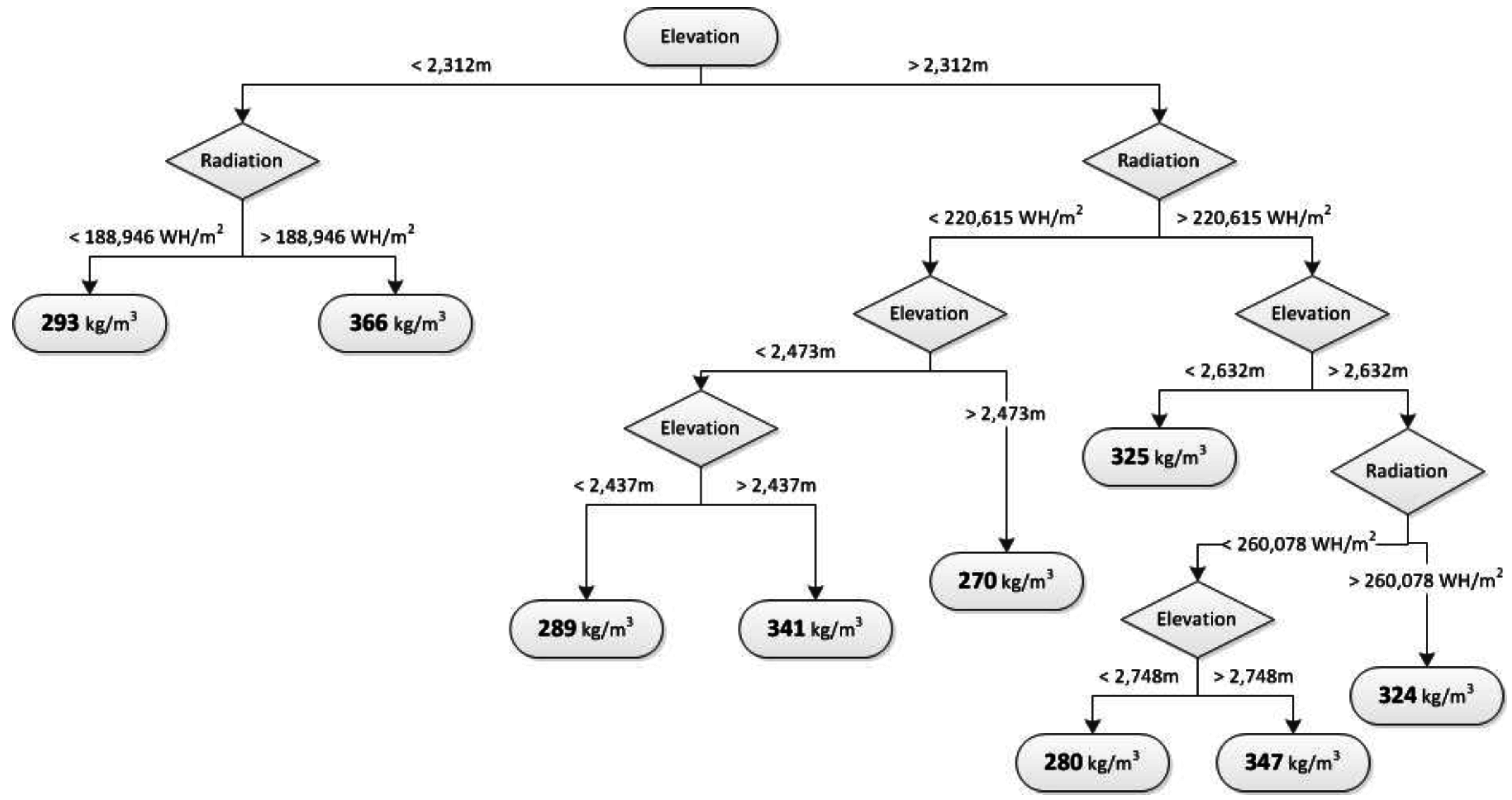
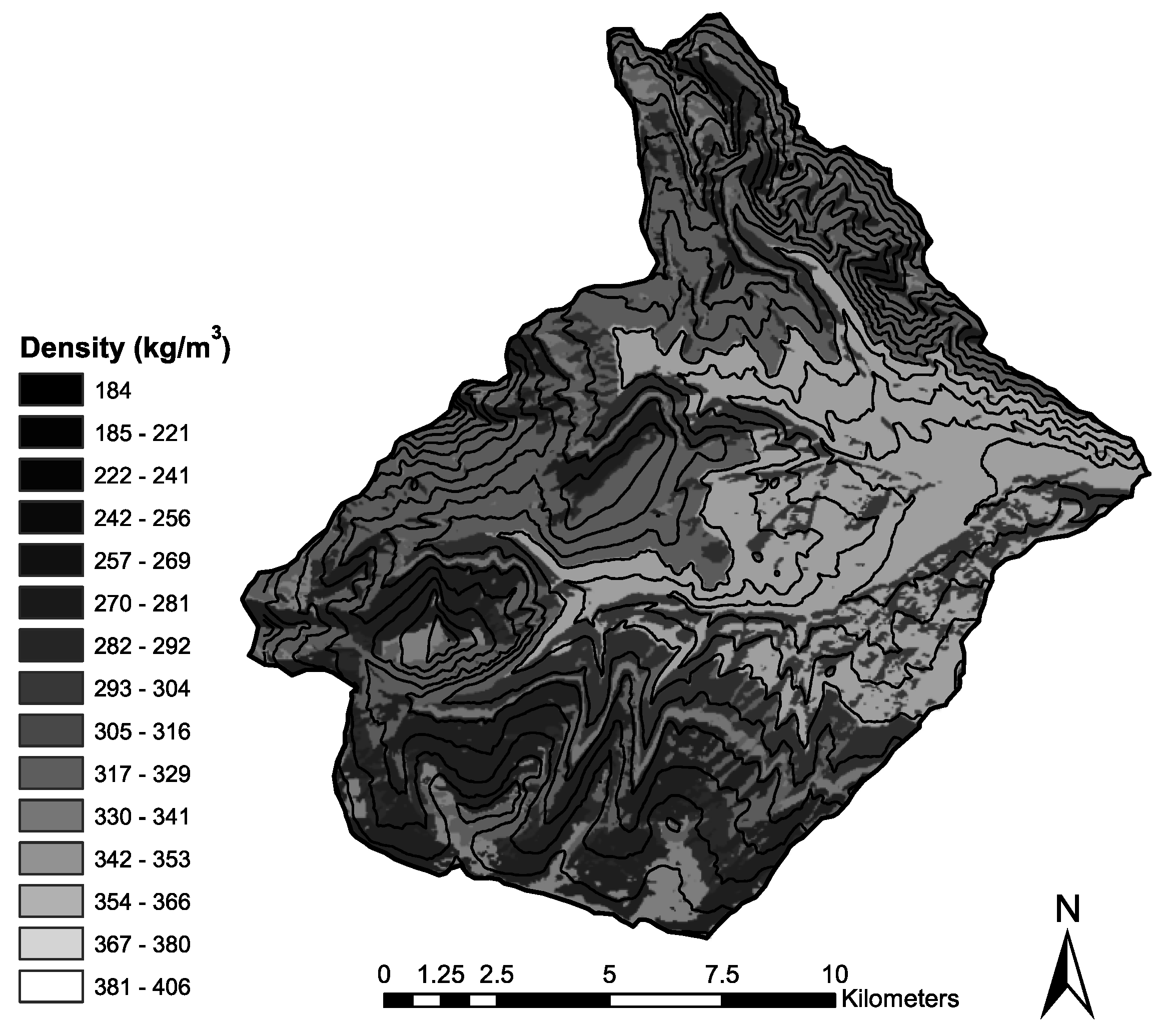
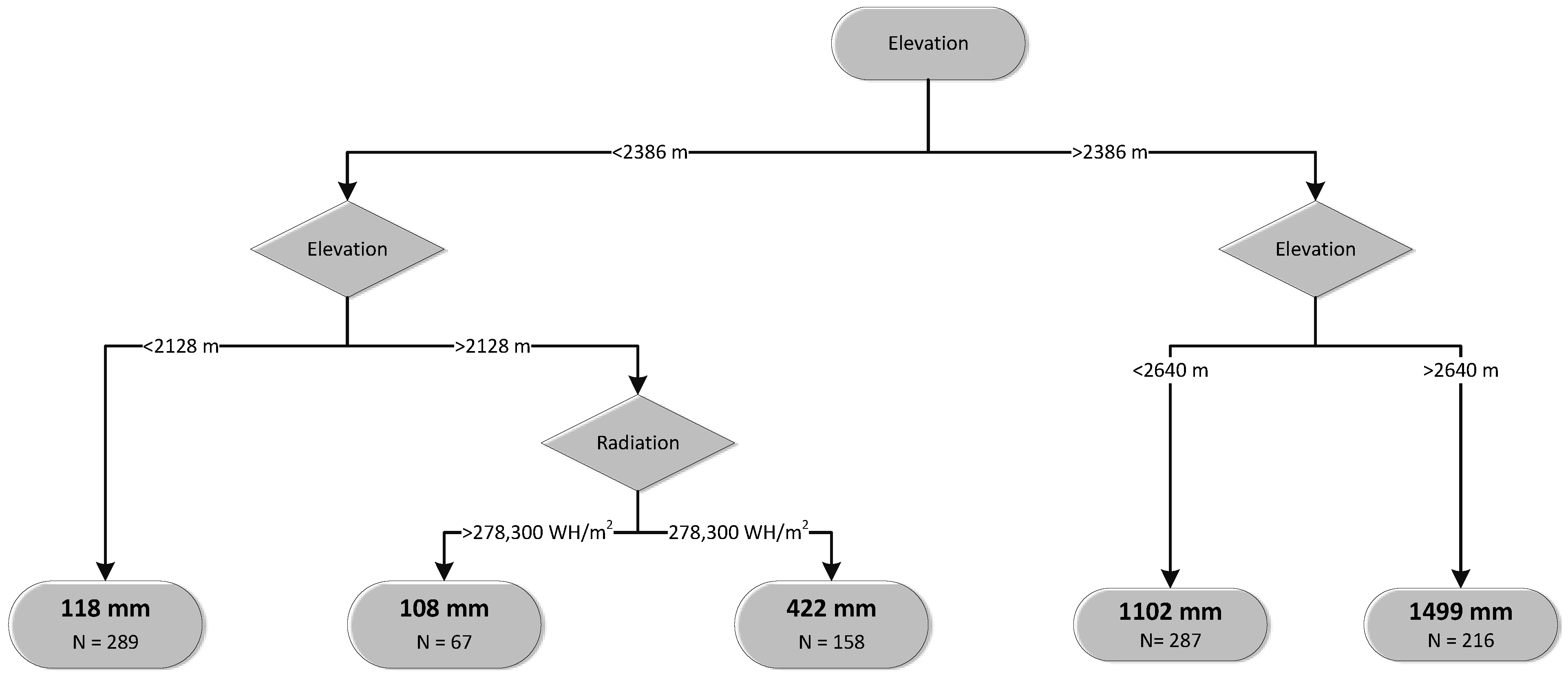
Snow density displayed considerable spatial variability throughout the West Fork Basin at the time of sampling, near peak accumulation. Significant correlations between the spatial distribution of density and the independent variables of elevation and incoming solar radiation were found using both regression tree and multiple linear regression modeling. Both methods showed density to decrease with increasing elevation, increase with increasing radiation, and vice versa. One split of the regression tree modeled a higher snow density with increasing elevation in the highest elevation areas, possibly due to increased wind compaction of snow in the exposed alpine portions of the basin.

Correlations with elevation and radiation are related to snow density, because they are both physically-based parameters that heavily influence the snowpack energy balance at any given point in a basin [4]. Snow density will increase with increased radiation, because the additional energy input can speed near-surface metamorphism, leading to larger grains, decreased pore space, and therefore, increased density. Additionally, areas that experience high radiation inputs will also be more likely to have snow surface melt introducing liquid water to the snowpack. This also increases density by filling pore space with liquid, as well as increasing grain sizes through liquid-ice interactions and enhanced metamorphism from the introduction of latent heat deeper in the pack as this water re-freezes [10]. Increasing elevation is related to decreased densities because of colder air temperatures due to adiabatic cooling and deeper snow depths requiring more energy input to substantially lower the average density through the entire snowpack profile. While Elder et al. [4] note slope angle to be a significant predictor of density because of its relation to wind transport and avalanching, direct statistical correlations between slope angle and density were not identified in this study.

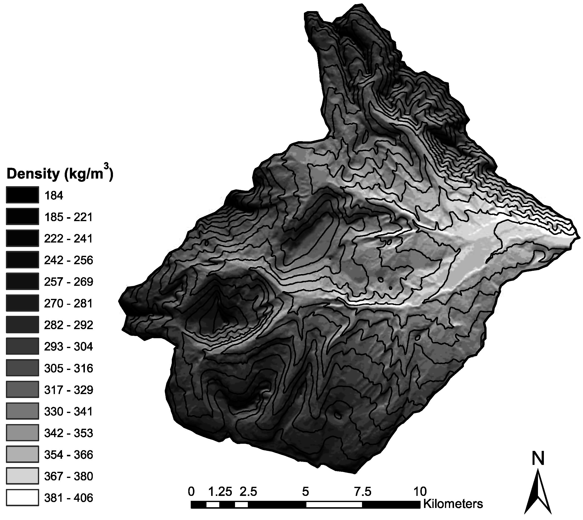
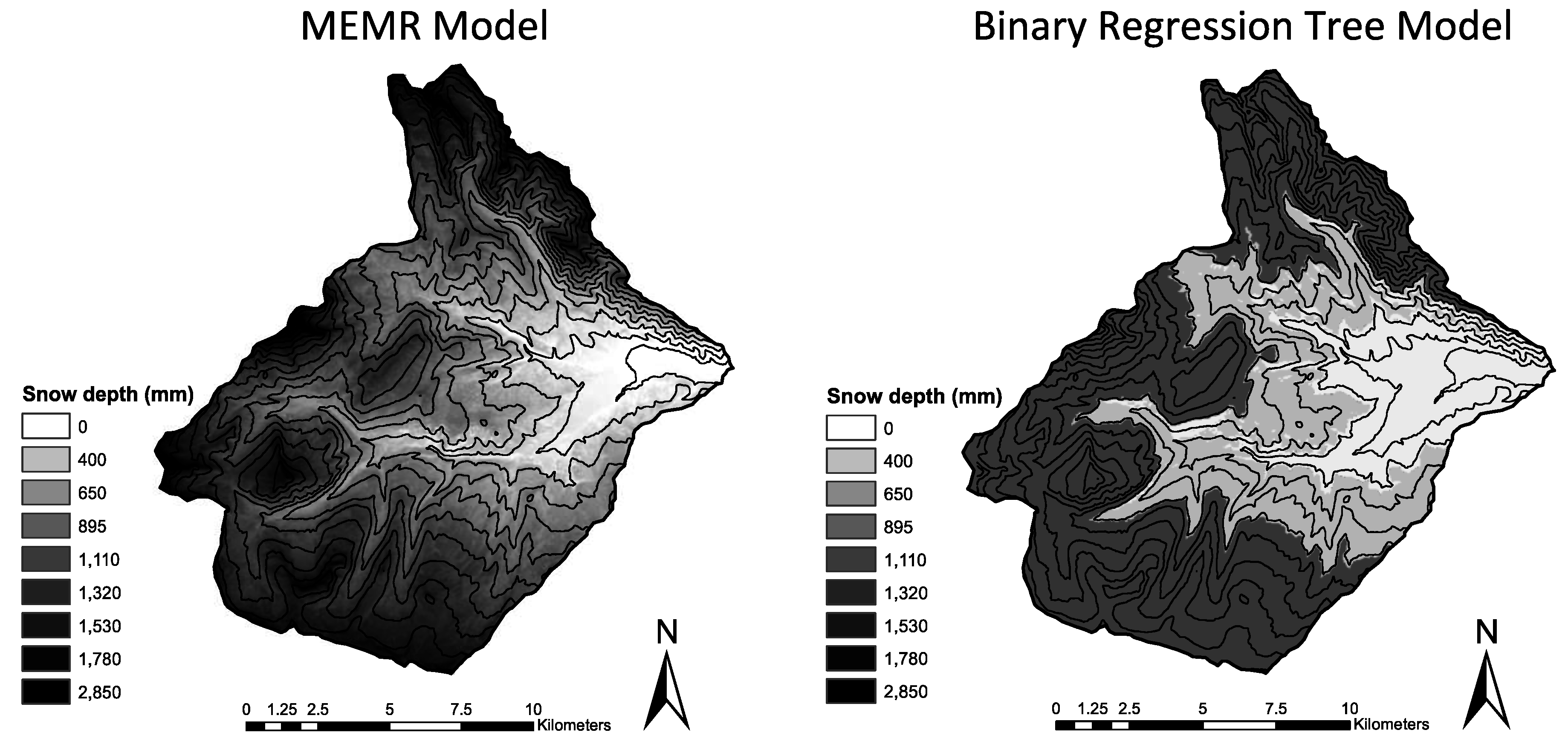
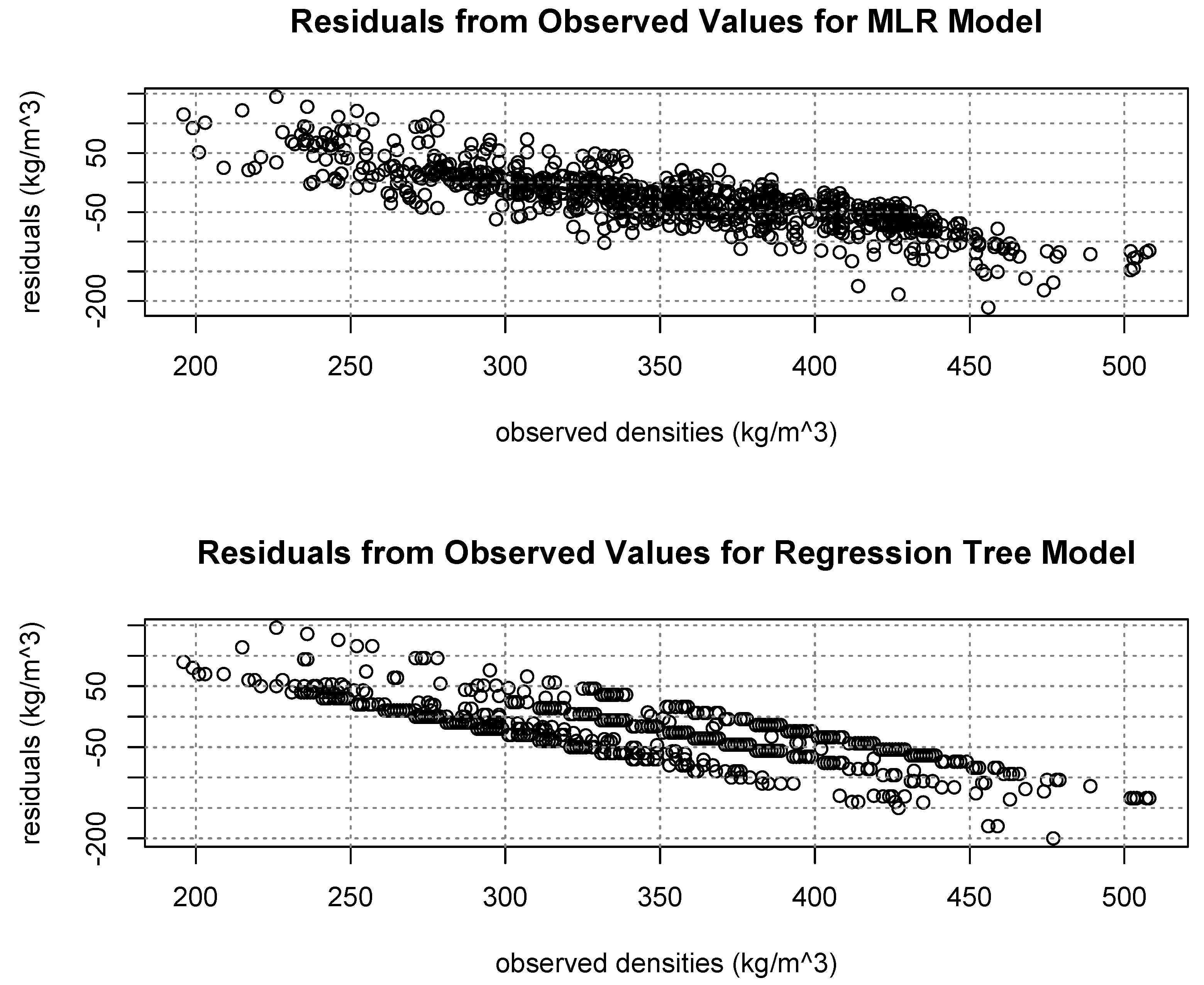
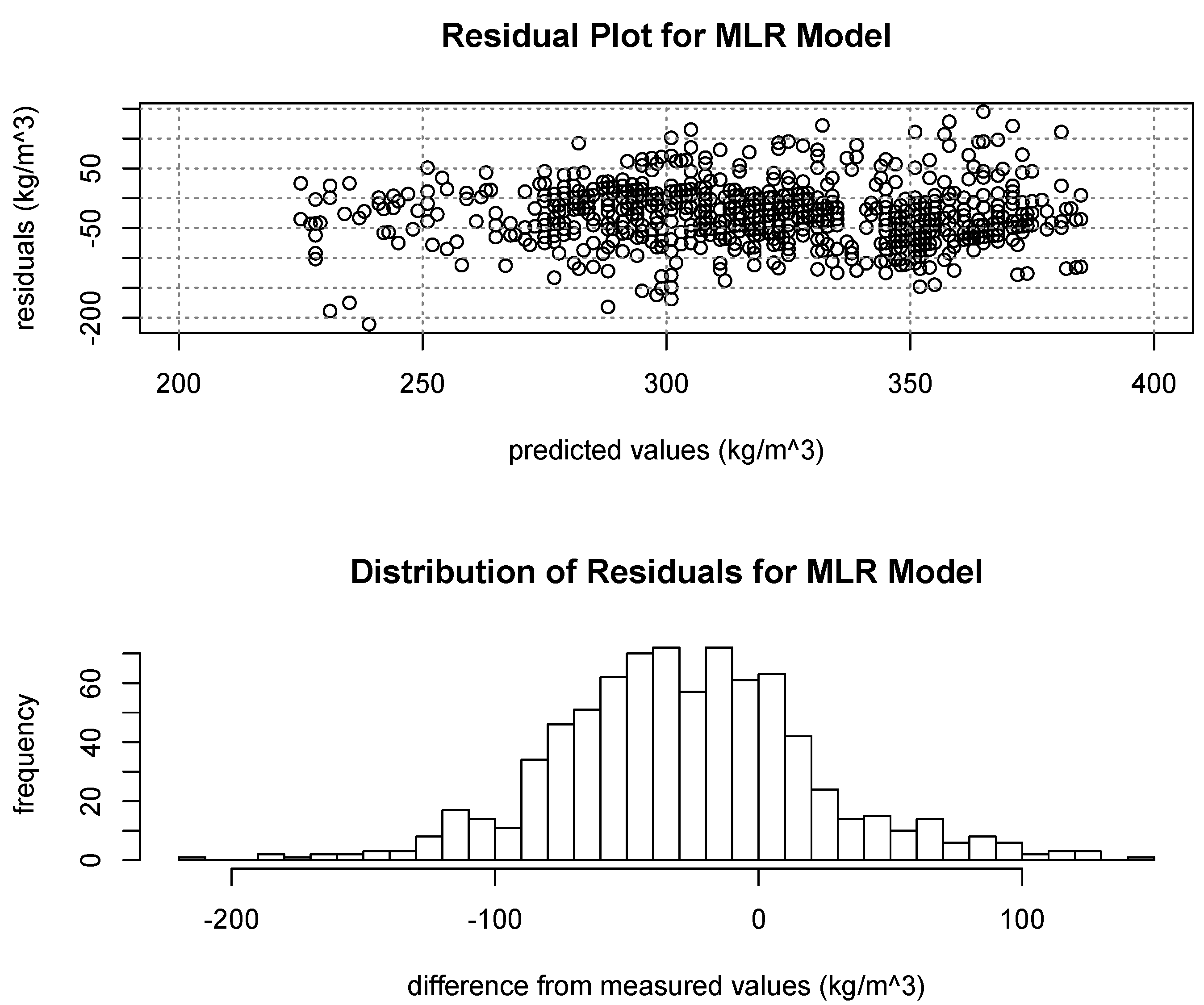
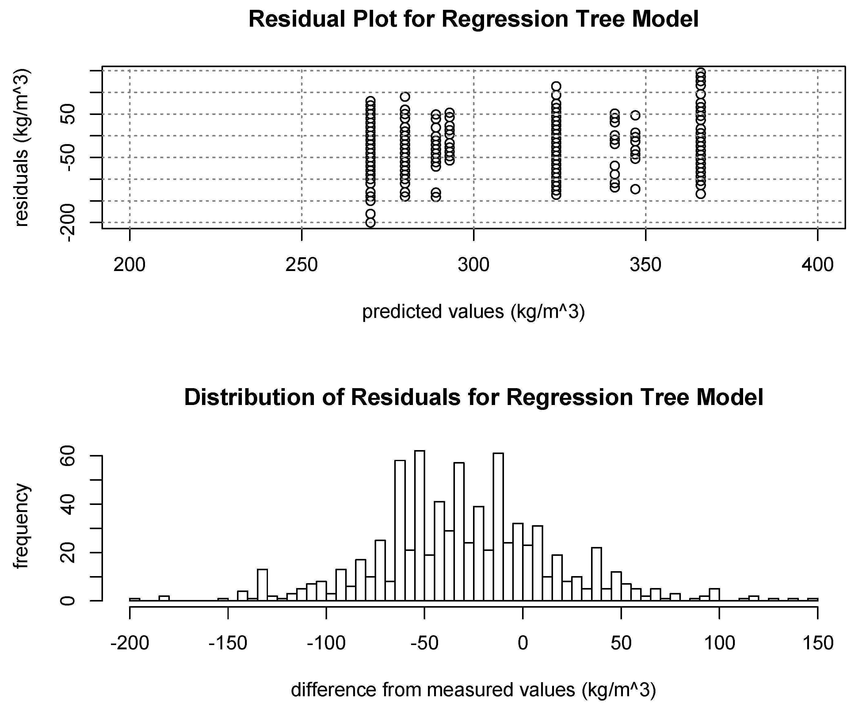
Both MLR and regression tree models were able to account for similar quantities of observed variation in snow density (39% and 41%, respectively), but provided notably different ranges of modeled values and spatial distributions. The MLR model provided a wider range of modeled densities and a continuous distribution of values, where the binary regression tree provided a narrower range and modeled nine discrete densities in its terminal nodes. The narrow range resulting from the regression tree model also emphasizes its inability to model outside of its observed range, which is another potential weakness of that model type. Even with the MLR model providing a wider range of estimates, both models estimated a narrower range of values than were measured in the field, resulting in a very similar pattern in the distribution of their residuals from observed values. The negative trend in Figure 12 displays how these narrower ranges (compared to observed values) led to over-estimation of the lowest measured densities and under-estimation of the highest measured densities.

Figure 12. Residuals from observed values showing general over-estimation for low densities and under-estimation for higher densities from both model types.

Figure 12. Residuals from observed values showing general over-estimation for low densities and under-estimation for higher densities from both model types.

The continuous distribution of the modeled values resulting from MLR more accurately captures the continuous distribution of values found in the field. It was also able to more accurately model the tails of the distribution, which the regression tree model did not. Based on the similar measure of model fit, it could be argued that either could be an appropriate representation of the spatial distribution of snow density throughout the West Fork Basin for the purpose of estimating total basin SWE. However, each model has its own advantages. The continuous nature and modeled tails of the distribution resulting from the MLR model does provide a more realistic representation of how snow densities are distributed in nature. The regression tree model, however (while only predicting nine discrete density values to be modeled throughout the basin), did model large changes in density over short distances due to changes in received radiation in a more realistic manner. Conversely, the modeling of the 349-kg/m³ values in the highest elevations is anomalous compared to the general observations throughout the basin. Overall, considering the benefits and disadvantages of both model types, the MLR model is considered to provide a more realistic representation of the spatial distribution of snow density in the West Fork Basin. Despite this, it is recommended that both methods (and potentially additional) be developed and evaluated to determine which model, or a combination thereof, provides the best representation of the spatial distribution of density for a given purpose.

A substantial body of work has been devoted to quantifying the spatial distribution of SWE in mountainous terrain, generally utilizing separate characterizations of depth and density to obtain SWE estimates. Some of these have used spatially-distributed models of density [4,5]. Others used spatially-uniform models and after finding poor density model results [8] or no significant correlations on which to model density [6]. Alternatively, Clark et al. [2] found minimal spatial variation in their density measurements and decided to focus their analysis on snow depth instead of SWE. The lack of significant correlations in these studies could be related to two primary factors. First, significant differences in density simply may not have existed in the field when data were collected for previous studies. Second, the quantity and/or spatial arrangement of samples acquired did not provide the pertinent data to statistically correlate associations that may have existed in the field [13,20].

Two primary factors likely contributed to the strong correlations between density and physiography in this study. First, both the elevation range (1580 m) and spatial extent (207 km²) of the West Fork Basin are notably larger than basins analyzed in previous field-based studies of SWE in mid-latitude mountainous regions (comparisons from Clark et al. [2]). This large extent and elevation range led to widely-varying characteristics of the snowpack near peak accumulation. Secondly, the acquisition of a large number of samples (n = 1017) in areas of the basin quantified to be physiographically representative of the whole and over a range of spatial scales allowed for differences in density to be statistically correlated to elevation and radiation.

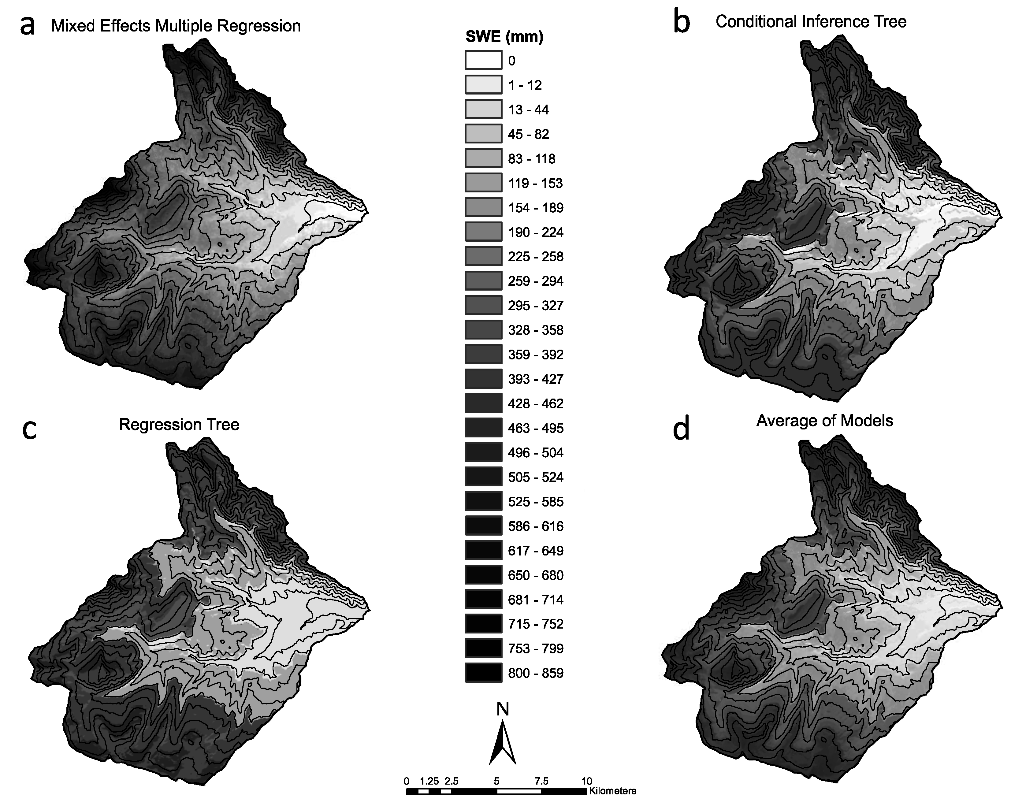
When using these spatially-distributed density models and a spatially-uniform parameterization of the average of measured densities to estimate total basin SWE, substantial differences in estimates were observed. When combined with the MEMR depth model, resulting SWE estimates had a range of 6.1% compared to the control models (in which estimates varied by ~1%), all estimating less SWE. Estimates of SWE utilizing the regression tree model for snow depth varied by 5.1%, with all estimates being higher than those derived from direct SWE measurements. The 14.1% total range of SWE estimates resulting from the six different combinations of depth and density parameterizations indicate that even with statistically-sound representations of the spatial distribution of density (and depth), model choice can still substantially influence SWE estimates. Because of these findings, it is recommended that if depth and density are to be combined to estimate SWE that a variety of spatial models (including spatially uniform, if desired) be analyzed to determine which are best for a given study. If multiple models are developed, estimates from the various models could also then be averaged or otherwise combined to obtain a final estimate of SWE, either as the total basin volume or a spatially-distributed representation.

Many important considerations exist when assessing the spatial distribution of snow density and comparing other studies that have done so. Snow density can be highly dynamic, spatially and temporally, especially through the transition from the accumulation to the ablation season. The annual timing, spatial patterns and rate of snowpack densification can vary substantially in different basins, mountain ranges and snow climates. In addition to differences that exist in the field, methods of sampling, data analysis and spatial modeling can also have an influence on the inferences obtained from any given body of work. This research emphasizes the importance of careful consideration of these factors, among others, when performing studies of the spatial distribution of snow density or SWE or analyzing the conclusions drawn by other research.

6. Conclusions

This study utilizes an original and unique dataset and analysis that shows that snow density can vary widely near the time of peak accumulation, and estimates of total basin SWE can vary widely from combining different models of the spatial distribution of depth and SWE. While it is more time efficient to sample for snow depth more intensely than for snow density or SWE directly, this can potentially be problematic for making accurate estimates of SWE, particularly near the time of peak accumulation when it is most important for water supply forecasting. The substantial differences that can occur in estimates of total basin SWE from varying the parameterizations of snow depth and snow density when making such estimates were quantified. The authors suggest that the importance of the spatial distribution of snow density and how it is represented in models should not be underestimated when using separate depth and density models to quantify the spatial distribution of SWE in mountainous terrain. This importance exists both with respect to ensuring density is sampled for in a manner that allows for the statistical capture of correlations that exist in the field and with respect to how the results are modeled spatially. Recommended future work includes continuing to improve the accuracy of spatially-distributed SWE models, as well as to expand the extent over which these are developed, from basin, to mountain range, to regional scales.