
Performance and Uncertainty Evaluation of Snow Models on Snowmelt Flow Simulations over a Nordic Catchment (Mistassibi, Canada)


Abstract
:1. Introduction
2. Experimental Design
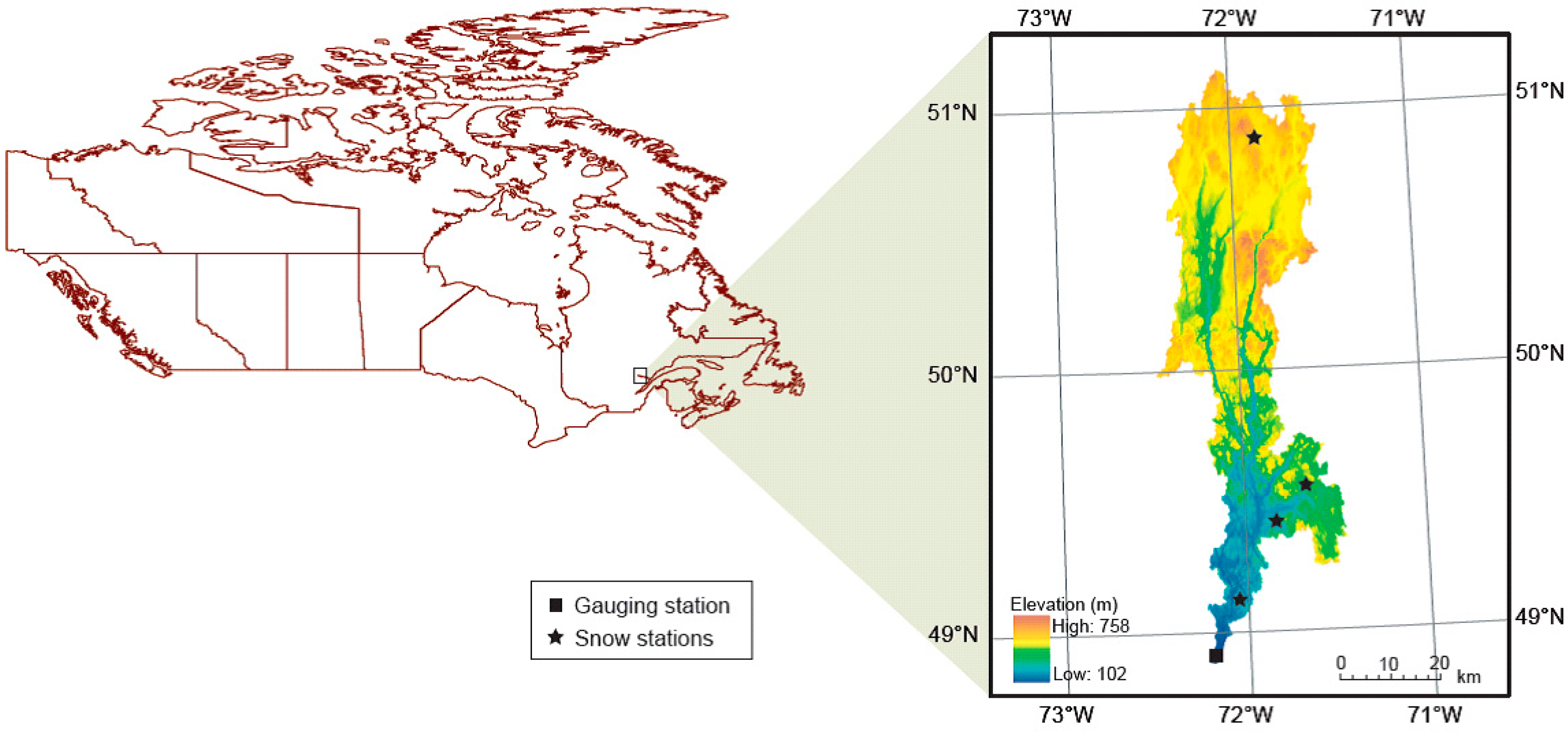
2.1. Study Area
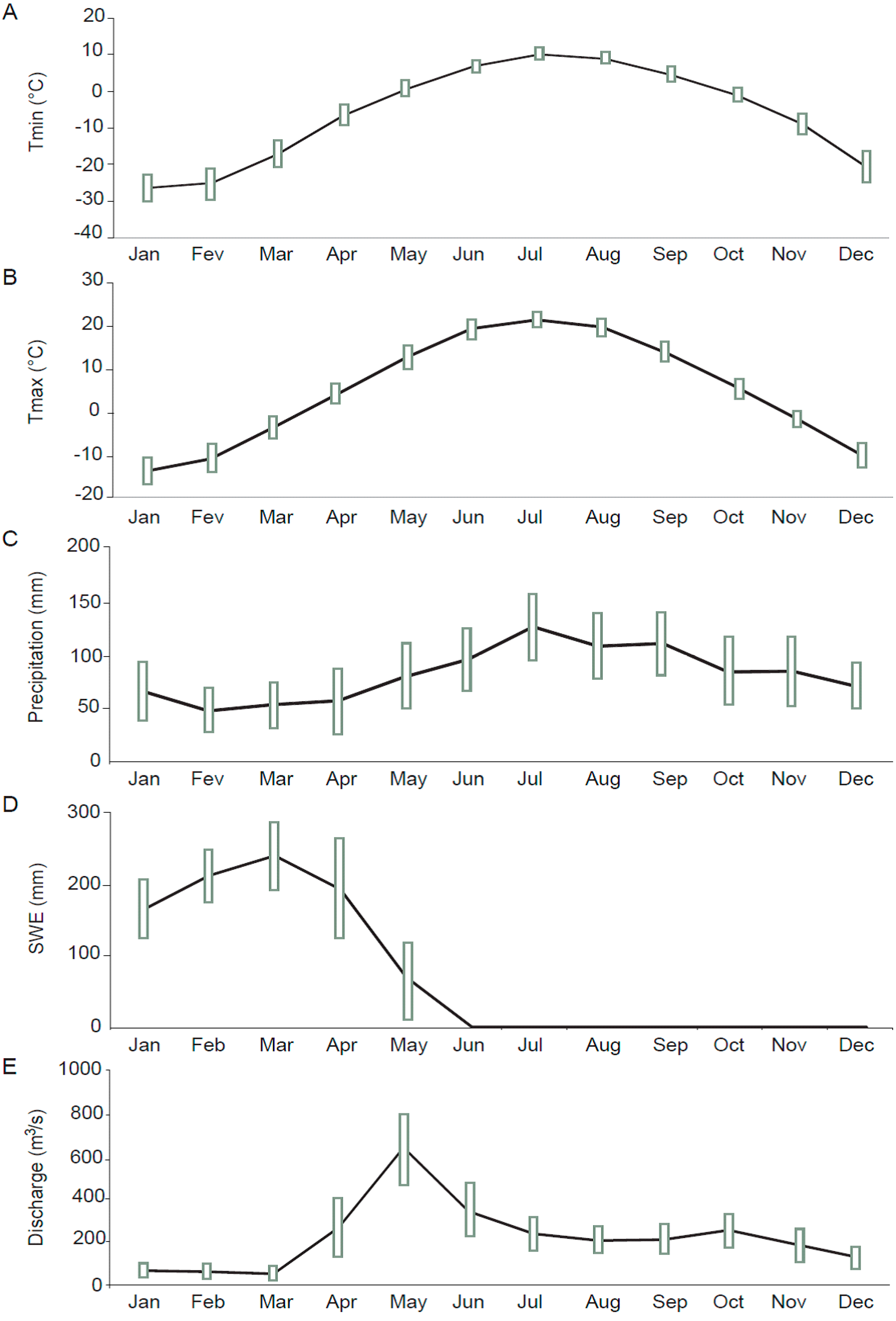
2.2. Data

| Mistassibi Basin | |
|---|---|
| Province | Quebec |
| Drainage area (km2) | 9320 |
| Elevation range (m) | 102–758 |
| Main land cover type | Forest (84%) |
| Hydrology | |
| Mean daily discharge (m3/s) | 285 |
| Minimum daily discharge (m3/s) | 25 |
| Maximum daily discharge (m3/s) | 1565 |
| Snow | |
| Mean daily SWE (mm) | 203 |
| Maximum daily SWE (mm) | 347 |
| Climate | |
| Annual average precipitation total (mm) | 978 |
| Annual daily temperature (°C) | |
| Min. | −46.1 |
| Max. | +35.1 |
| Mean | −0.9 |
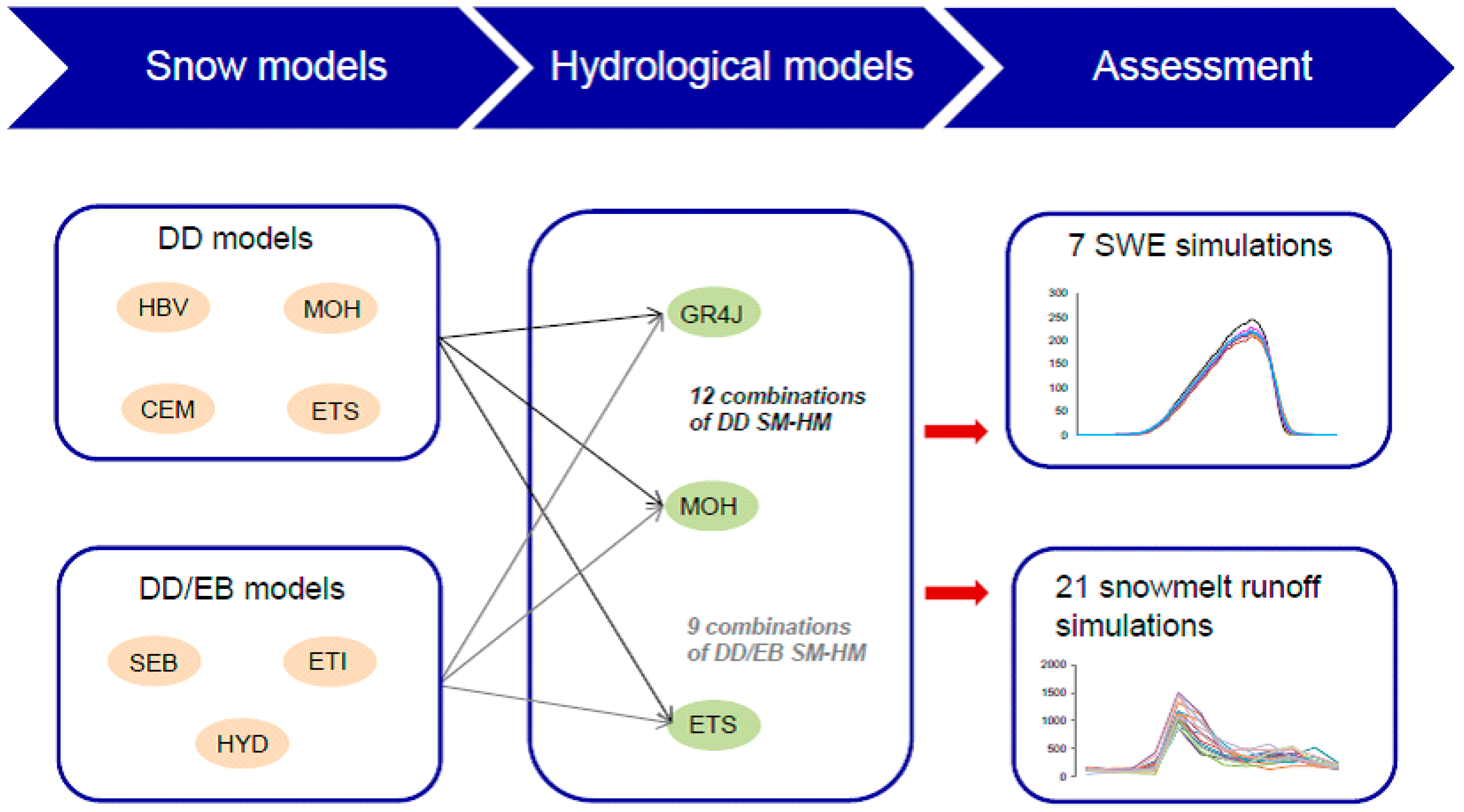
3 The Multi-Model Approach

3.1. Description of Snow Models
| Model Type | Input Data a | Snow Parameters | State Variables | |
|---|---|---|---|---|
| MOHYSE (MOH) | Degree-day | T, P | 2 | 1 |
| HBV (HBV) | Degree-day | T, P | 3 | 2 |
| CEMANEIGE (CEM) | Degree-day | T, P | 2 | 2 |
| HMETS (ETS) | Degree-day | T, P | 10 | 5 |
| HYDROTEL (HYD) | Degree-day/energy balance | T, P | 5 | 4 |
| SEB (SEB) | Degree-day/energy balance | T, P, ISR, α | 2 | 1 |
| ETI (ETI) | Degree-day/energy balance | T, P, ISR, α | 2 | 1 |
3.1.1. Degree-Day Models
MOHYSE
HBV
CEMANEIGE
HMETS
3.1.2. Mixed Degree-Day and Energy Balance Models
HYDROTEL
SEB
ETI
3.2. Description of Hydrological Models
3.2.1. MOHYSE
3.2.2. HMETS
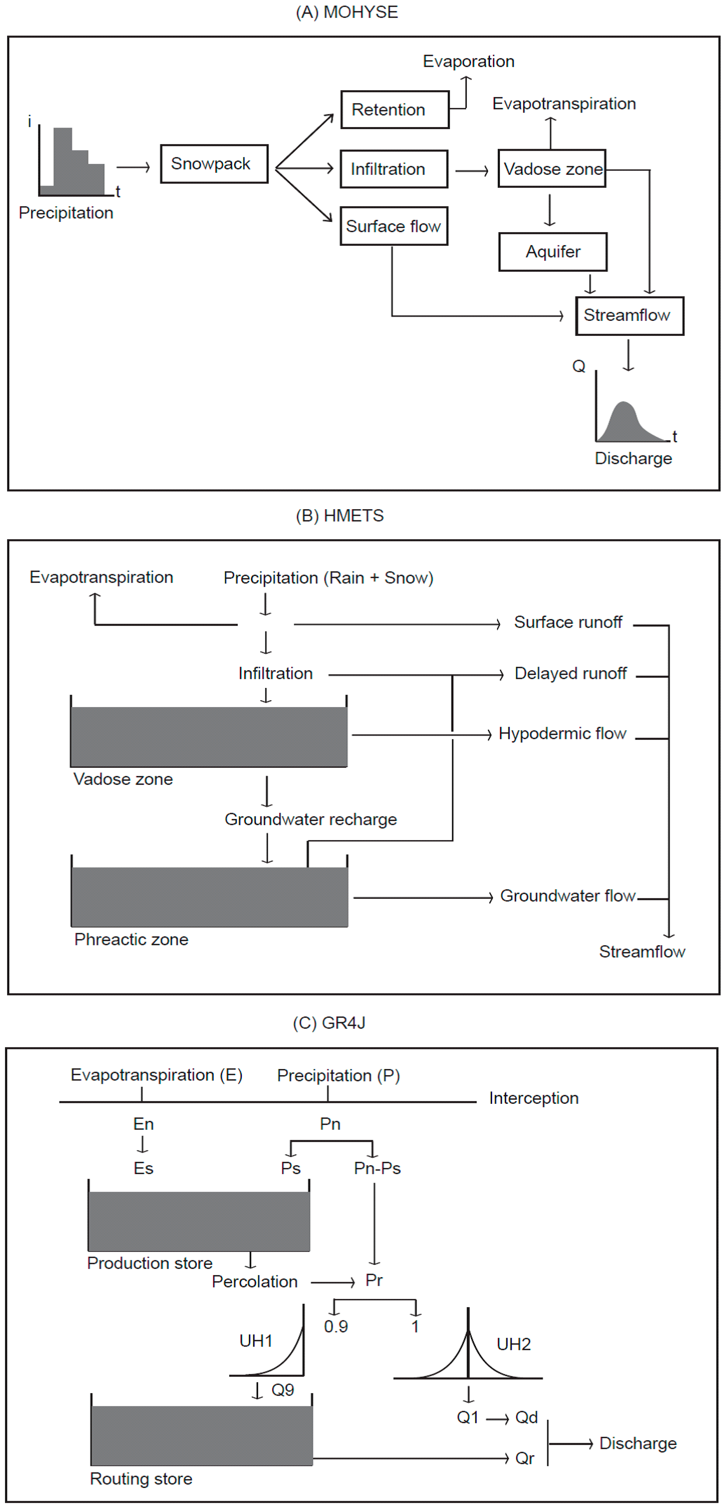
3.2.3. GR4J
3.3. Models Calibration Strategy and Evaluation Method
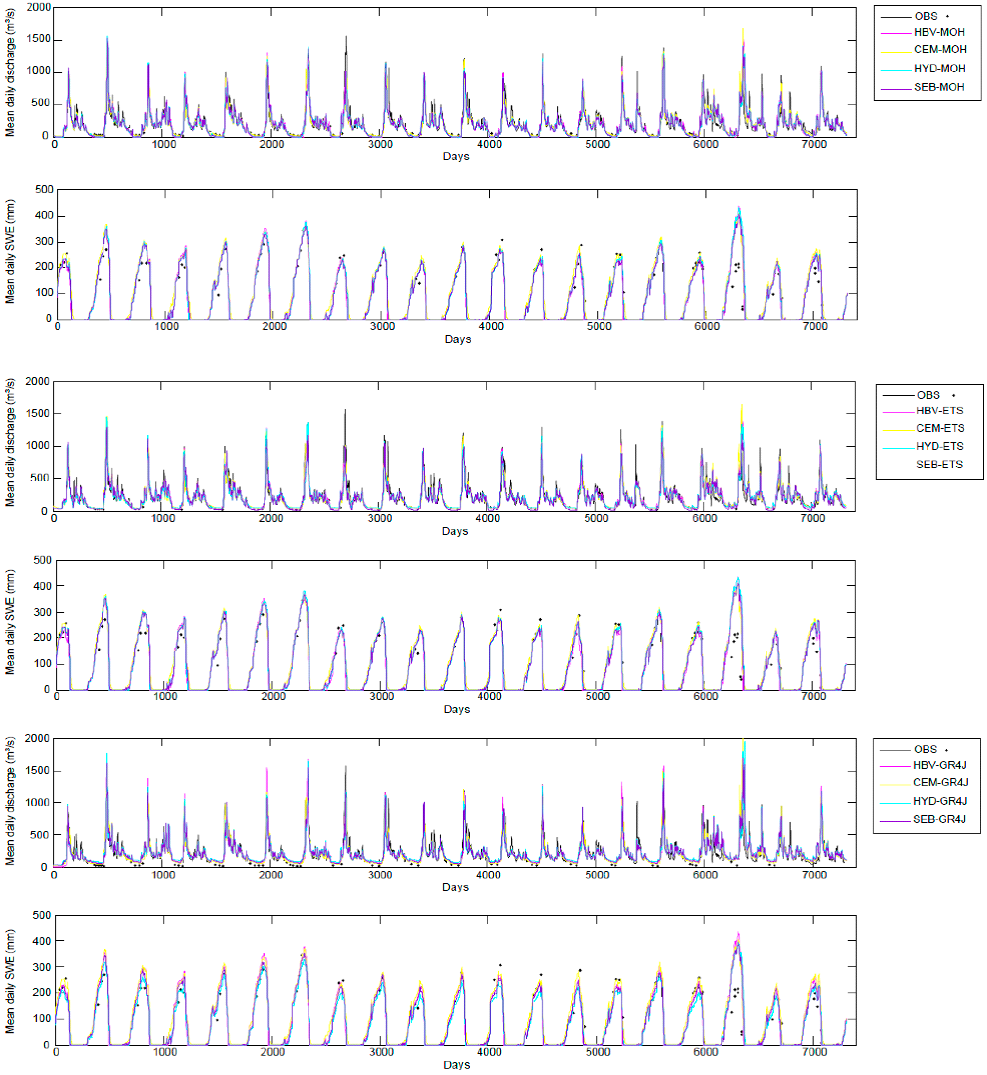
4 Results
4.1. Performance of the SM-HM Combinations in Snowmelt Flows
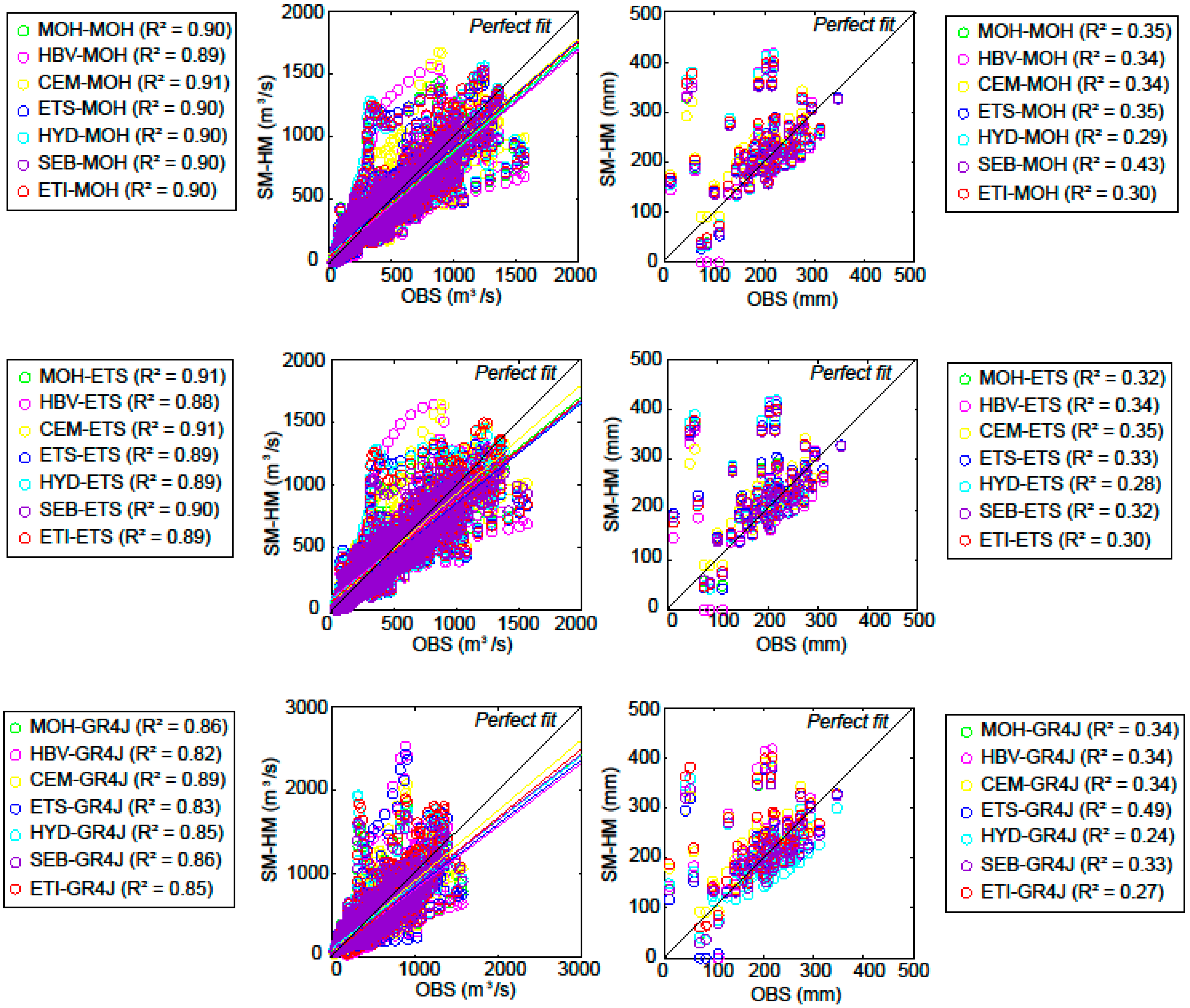
4.1.1. Calibration


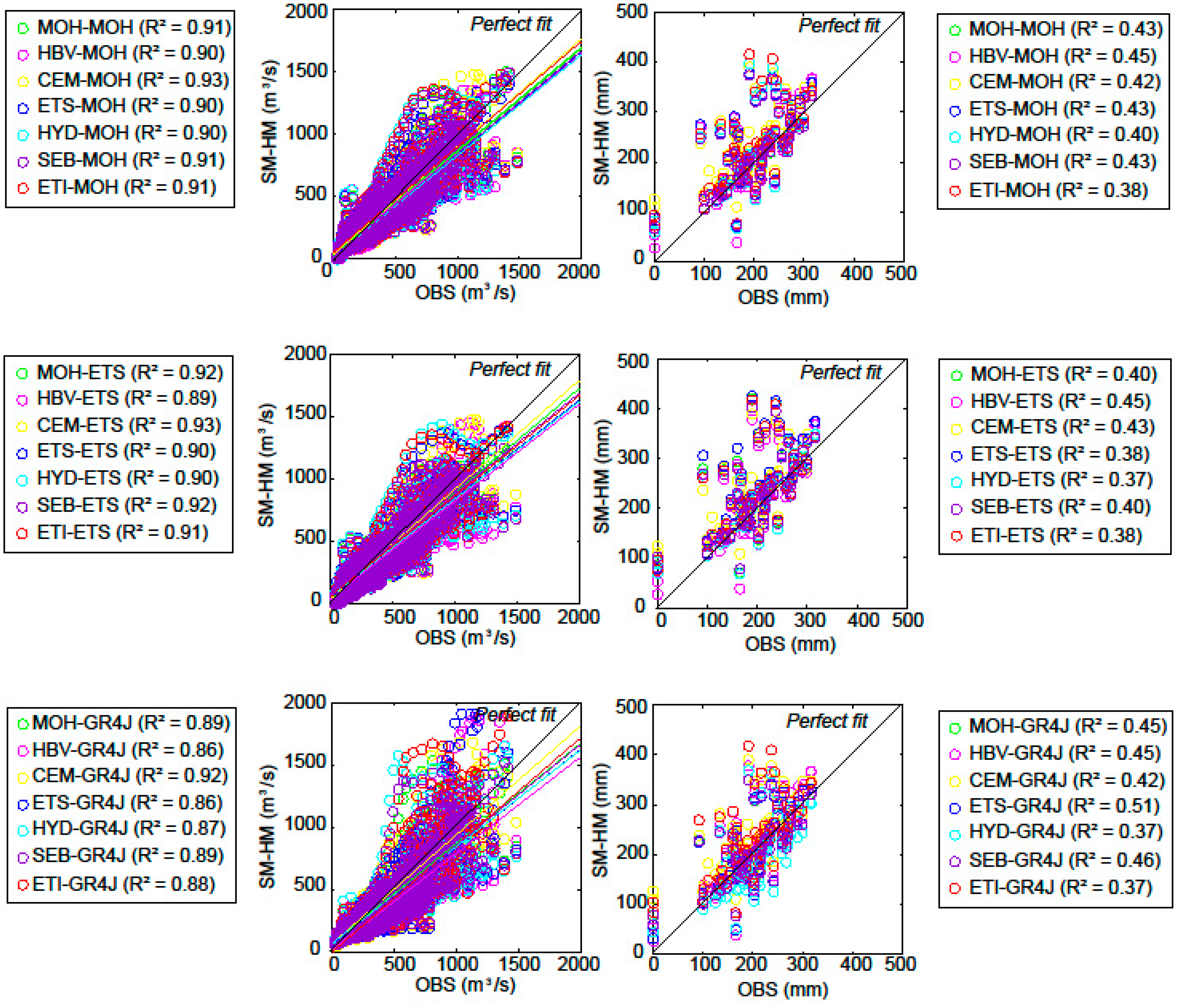
4.1.2. Validation
| Calibration | Validation | |||||
|---|---|---|---|---|---|---|
| NS | R2 | DV (%) | NS | R2 | DV (%) | |
| MOH-MOH | 0.81 | 0.90 | −0.57 | 0.82 | 0.91 | −4.27 |
| HBV-MOH | 0.78 | 0.89 | 0.07 | 0.80 | 0.90 | −4.13 |
| CEM-MOH | 0.83 | 0.91 | −0.90 | 0.87 | 0.93 | −3.54 |
| ETS-MOH | 0.81 | 0.90 | −0.48 | 0.80 | 0.90 | −4.54 |
| HYD-MOH | 0.80 | 0.90 | −0.96 | 0.80 | 0.90 | −4.97 |
| SEB-MOH | 0.81 | 0.90 | −0.50 | 0.82 | 0.91 | −4.27 |
| ETI-MOH | 0.80 | 0.90 | −1.47 | 0.82 | 0.91 | −4.64 |
| MOH-ETS | 0.82 | 0.91 | −0.52 | 0.85 | 0.92 | −2.74 |
| HBV-ETS | 0.77 | 0.88 | 0.43 | 0.79 | 0.89 | −3.63 |
| CEM-ETS | 0.83 | 0.91 | −0.26 | 0.87 | 0.93 | −3.47 |
| ETS-ETS | 0.80 | 0.89 | −1.60 | 0.81 | 0.90 | −3.99 |
| HYD-ETS | 0.79 | 0.89 | −0.44 | 0.80 | 0.90 | −3.84 |
| SEB-ETS | 0.82 | 0.90 | −0.80 | 0.84 | 0.92 | −3.58 |
| ETI-ETS | 0.80 | 0.89 | 0.05 | 0.83 | 0.91 | −2.95 |
| MOH-GR4J | 0.74 | 0.86 | −0.54 | 0.77 | 0.89 | −5.34 |
| HBV-GR4J | 0.66 | 0.82 | −1.40 | 0.73 | 0.86 | −5.33 |
| CEM-GR4J | 0.79 | 0.89 | −1.06 | 0.85 | 0.92 | −4.79 |
| ETS-GR4J | 0.67 | 0.83 | 1.84 | 0.74 | 0.86 | −2.73 |
| HYD-GR4J | 0.71 | 0.85 | −0.43 | 0.75 | 0.87 | −5.22 |
| SEB-GR4J | 0.74 | 0.86 | −0.59 | 0.79 | 0.89 | −5.44 |
| ETI-GR4J | 0.71 | 0.85 | −1.82 | 0.76 | 0.88 | −5.00 |
4.2. Uncertainty Analysis
4.2.1. Uncertainty of Snow Models on Snowmelt Flows

4.2.2. Uncertainty of Hydrological Models on Snowmelt Flows
5. Discussion
6. Conclusions
- (1)
- For the study period and the basin considered, the 21 SM-HM combinations have similar satisfactory discharge simulation performances during the calibration and validation periods, with R2 values above 0.8 and NS values above 0.7.
- (2)
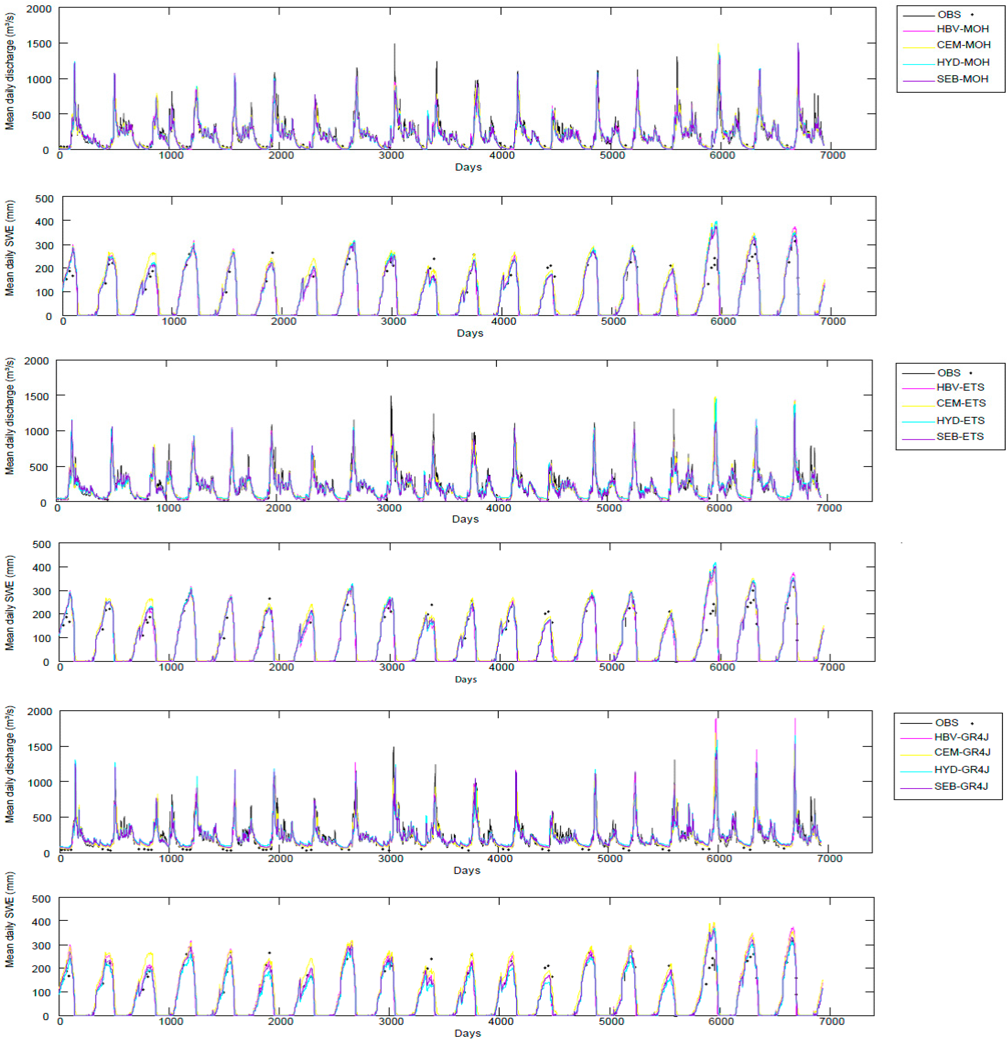
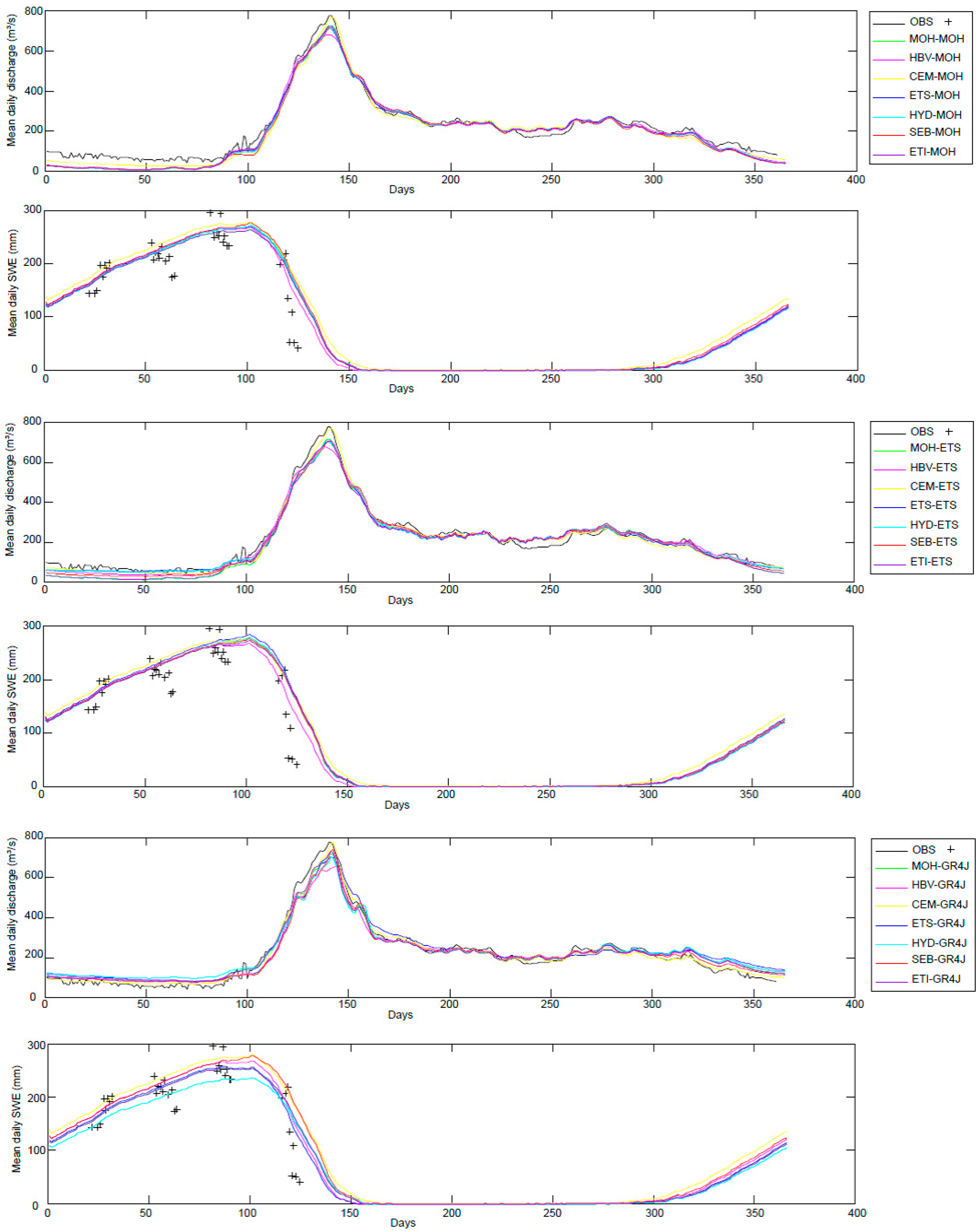
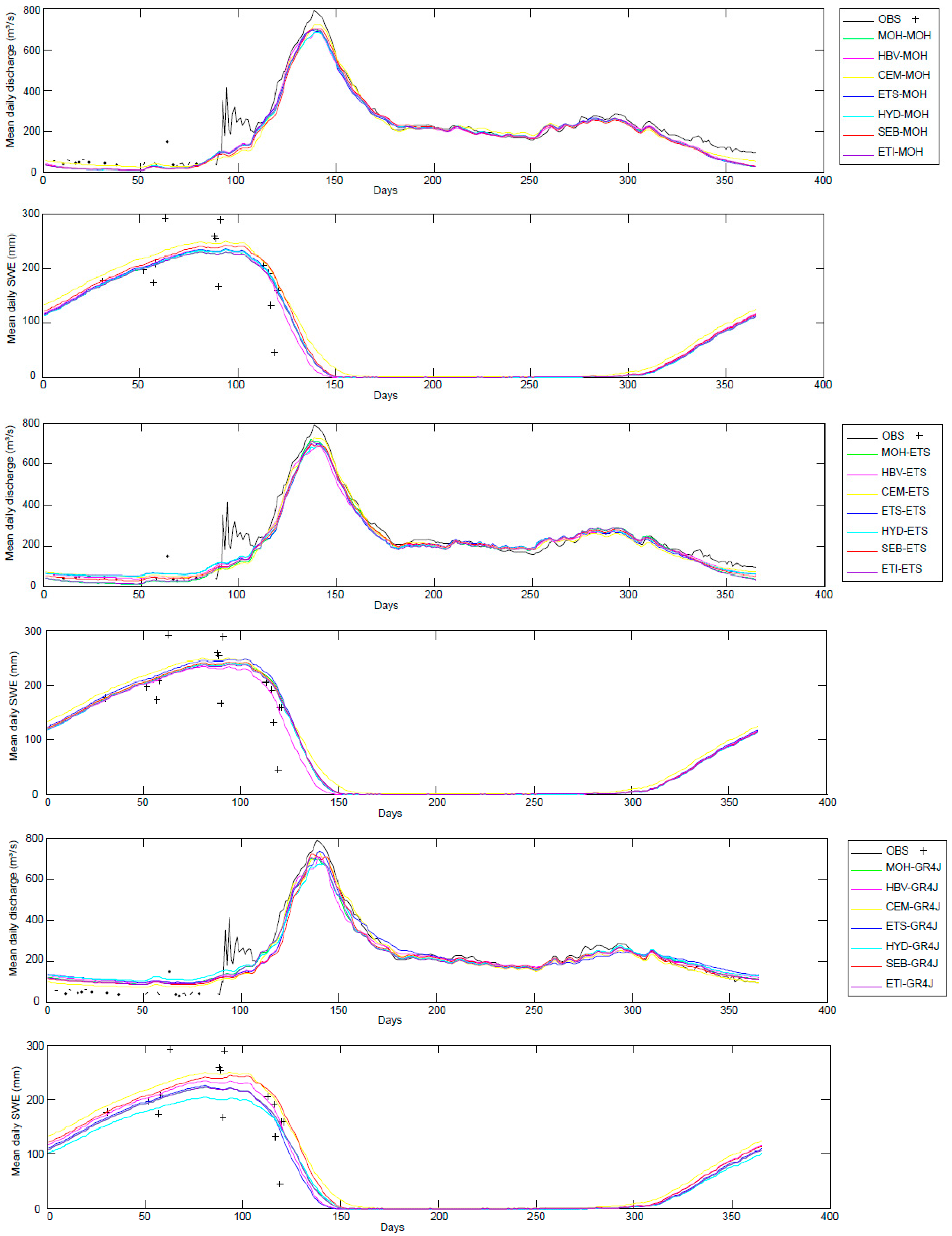
- The ensemble of 21 SM-HM combinations simulates daily discharges and SWEs that follow the trends of observed values in the Mistassibi Basin. All the SM-HM combinations underestimate the spring-snowmelt-generated peak flow due to the underestimation of the peak snow accumulation by the SMs.
- (3)
- Both the DD SM-HM and DD/EB SM-HM approaches agree fairly well regarding the simulation of snowmelt flows over the Mistassibi Basin. This level of agreement implies that the simple DD SM models can be considered to be a tool as effective as the more sophisticated DD/EB SM models for simulating snowmelt flows at the catchment scale.
- (4)
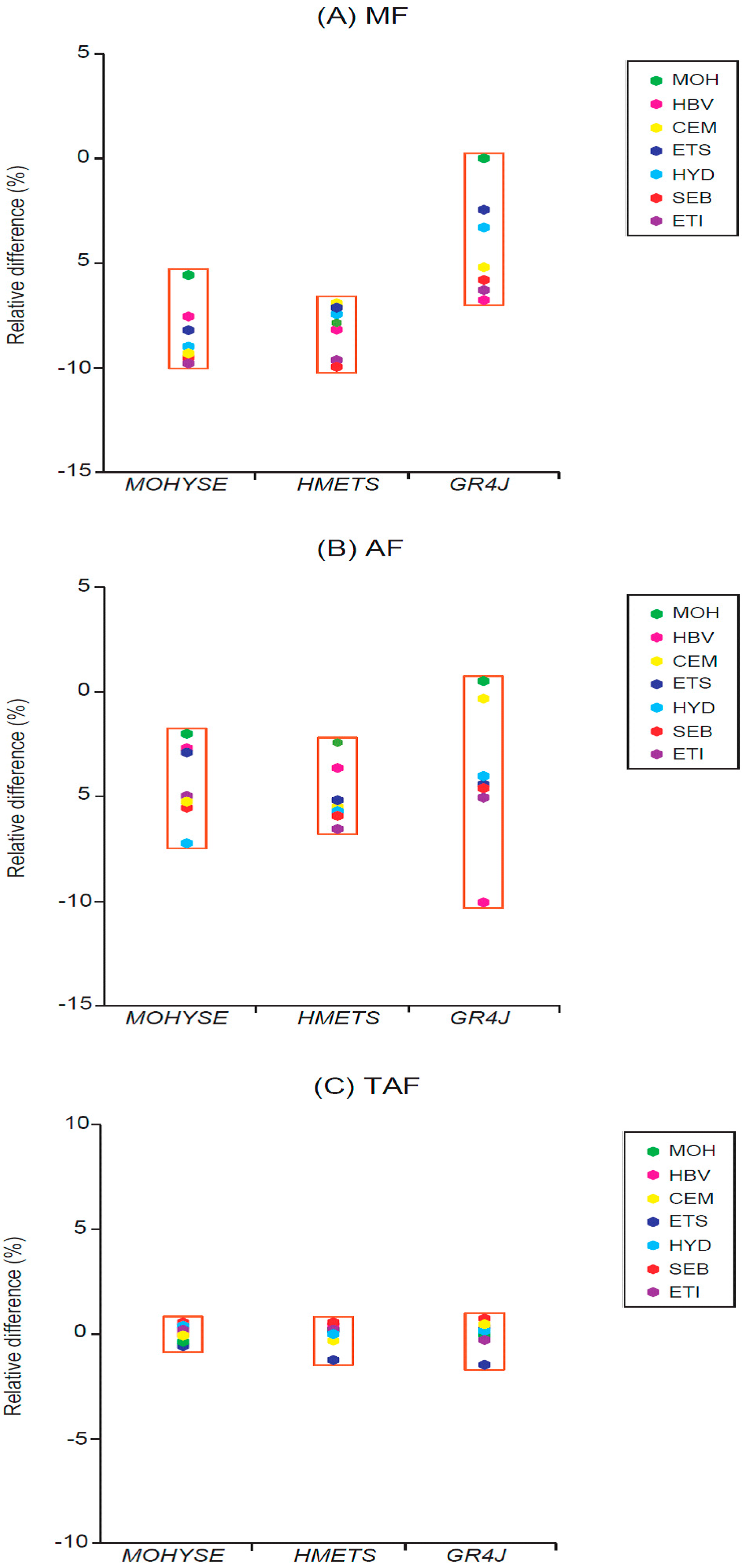
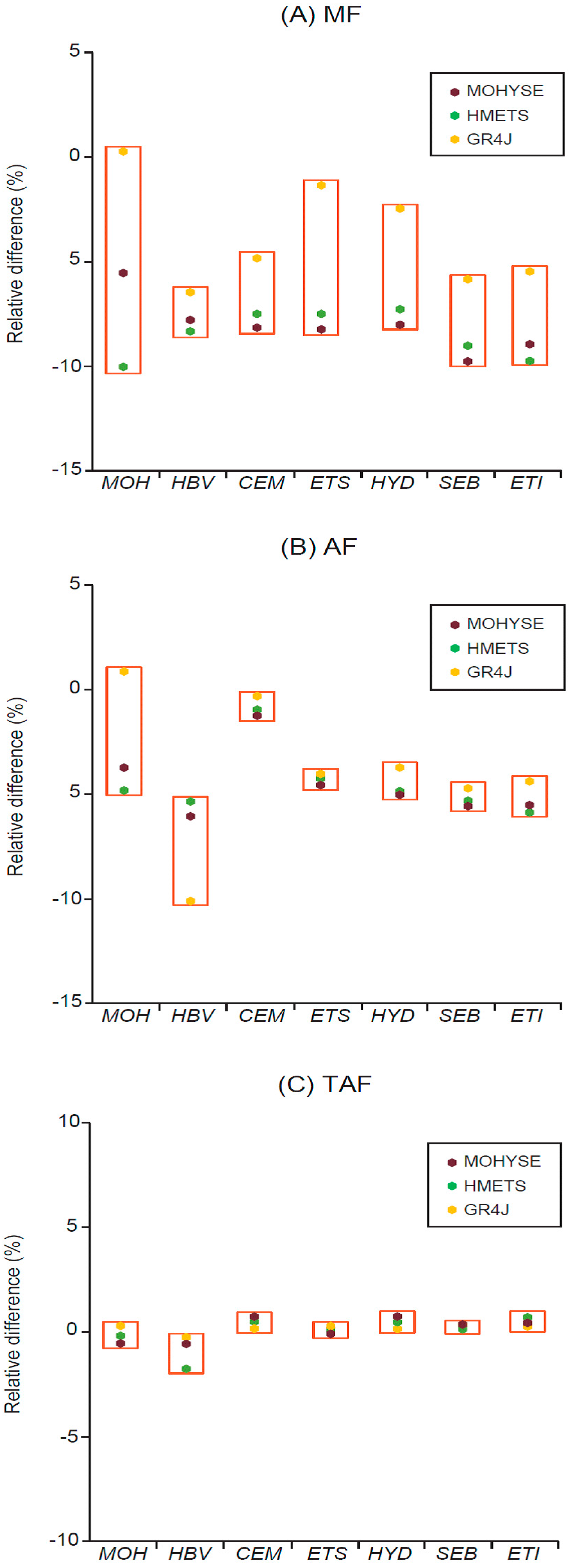
- The present investigation has permitted an estimation of the source of uncertainty associated to model structure in discharge simulations. The analysis of specific hydrologic indicators shows that the main uncertainties result from the hydrological models followed by the snow models. The uncertainty related to the choice of the given HM cannot be neglected in snow hydrological studies. The selection of the SM plays a more important role than the choice of the SM approach (DD versus DD/EB) in simulating snowmelt flows.
Acknowledgments
Author Contributions
Conflicts of Interest
References
- Wagener, T.; Gupta, H.V. Model identification for hydrological forecasting under uncertainty. Stochastic Environ. Res. Risk. Assess. 2005. [Google Scholar] [CrossRef]
- Georgakakos, K.P.; Seo, D.J.; Gupta, H.V.; Schaake, J.; Butts, M.B. Towards the characterization of streamflow simulation uncertainty through multimodel ensembles. J. Hydrol. 2004, 298, 222–241. [Google Scholar] [CrossRef]
- Liu, Y.; Gupta, H.V. Uncertainty in hydrologic modeling: Toward an integrated data assimilation framework. Water Resour. Res. 2007. [Google Scholar] [CrossRef]
- Najafi, M.R.; Moradkhani, H.; Jung, I.W. Assessing the uncertainties of hydrologic model selection in climate change impact studies. Hydrol. Processes 2011, 25, 2814–2826. [Google Scholar] [CrossRef]
- Poulin, A.; Brissette, F.; Leconte, R.; Arsenault, R.; Malo, J.S. Uncertainty of hydrological modelling in climate change impact studies in a Canadian, snow-dominated river basin. J. Hydrol. 2011, 409, 626–636. [Google Scholar] [CrossRef]
- Neitsch, S.L.; Arnold, J.G.; Kiniry, J.R.; Williams, J.R. Soil and Water Assessment Tool (SWAT) Theoretical Documentation; Blackland Research Center, Texas Agricultural Experiment Station: Temple, TX, USA, 2001; p. 781. [Google Scholar]
- Martinec, J.; Rango, A.; Roberts, R.T. Snowmelt Runoff Model (SRM) User’s Manual; New Mexico State University: Las Cruces, New Mexico, 2008; p. 175. [Google Scholar]
- Rango, A.; Dewalle, D. Snowmelt-runoff model (SRM). In Principles of Snow Hydrology; Dewalle, D., Rango, A., Eds.; Cambridge University Press: Cambridge, NY, USA, 2008; pp. 306–364. [Google Scholar]
- Roy, A.; Royer, A.; Turcotte, R. Improvement of springtime streamflow in a boreal environment by incorporing snow-covered area derived from remote sensing data. J. Hydrol. 2010, 390, 35–44. [Google Scholar] [CrossRef]
- Mauser, W.; Bach, H. PROMET—Large scale distributed hydrological modelling to study the impact of climate change on the water flows of mountain watersheds. J. Hydrol. 2009, 376, 362–377. [Google Scholar] [CrossRef]
- Oreiller, M.; Nadeau, D.F.; Minville, M.; Rousseau, A.N. Modelling snow water equivalent and spring runoff in a boreal watershed, James Bay, Canada. Hydrol. Processes 2014, 28, 5991–6005. [Google Scholar] [CrossRef]
- Pellicciotti, F.; Brock, B.; Strasser, U.; Burlando, P.; Funk, M.; Corripio, J. An enhanced temperature-index glacier melt model including the shortwave radiation balance: Development and testing for Haut Glacier d’Arolla, Switzerland. J. Glaciol. 2005, 51, 573–587. [Google Scholar] [CrossRef]
- Brun, E.; Martin, E.; Simon, V.; Gendre, C.; Coleou, C. An energy andmass model of snow-cover suitable for operational avalanche forecasting. J. Glaciol. 1989, 35, 333–342. [Google Scholar]
- Bartelt, P.; Lehning, M. A physical SNOWPACK model for the Swissavalanche warning: Part I: Numerical model. Cold Reg. Sci. Technol. 2002, 35, 123–145. [Google Scholar] [CrossRef]
- Pellicciotti, F.; Helbing, J.; Rivera, A.; Favier, V.; Corripio, J.; Araos, J.; Sicart, J.E.; Carenzo, M. A study of the energy balance and melt regime on Juncal Norte Glacier, semi-arid Andes of central Chile, using melt models of different complexity. Hydrol. Processes 2008, 22, 3980–3997. [Google Scholar] [CrossRef]
- Jain, S.K.; Goswami, A.; Saraf, A.K. Snowmelt runoff modelling in a Himalayan Basin with the aid of satellite data. Int. J. Remote Sens. 2010, 31, 6603–6618. [Google Scholar] [CrossRef]
- Debele, B.; Srinivasan, R.; Gosain, A.K. Comparison of Process- Based and Temperature-Index Snowmelt Modeling in SWAT. Water Resour. Manag. 2009, 24, 1065–1088. [Google Scholar] [CrossRef]
- Troin, M.; Caya, D. Evaluating the SWAT’s snow hydrology over a Northern Quebec watershed. Hydrol. Processes 2014, 28, 1858–1873. [Google Scholar] [CrossRef]
- Kay, A.L.; Crooks, S.M. An investigation of the effect of transient climate change on snowmelt, flood frequency and timing in northern Britain. Int. J. Climatol. 2014, 34, 3368–3381. [Google Scholar] [CrossRef]
- Panday, P.K.; Williams, C.A.; Frey, K.E.; Brown, M.E. Application and evaluation of a snowmelt runoff model in the Tamor River basin, Eastern Himalaya using a Markov Chain Monte Carlo (MCMC) data assimilation approach. Hydrol. Processes 2014, 28, 5337–5353. [Google Scholar] [CrossRef]
- Troin, M.; Caya, D.; Velázquez, J.A.; Brissette, F. Hydrological response to dynamical downscaling of climate model outputs: A case study for western and eastern Canada snowmelt-dominated catchments. J. Hydrol. 2015, 4, 595–610. [Google Scholar] [CrossRef]
- Hock, R. Temperature index melt modelling in mountain areas. J. Hydrol. 2003, 282, 104–115. [Google Scholar] [CrossRef]
- Troin, M.; Poulin, A.; Baraer, M.; Brissette, F. Comparing snow models under current and future climates over three Nordic catchments: Uncertainties and implications for hydrological impact studies. J. Hydrol. 2015. submitted. [Google Scholar]
- Hutchinson, M.F.; McKenney, D.W.; Lawrence, K.; Pedlar, J.H.; Hopkinson, R.F.; Milewska, E.; Papadopol, P. Development and testing of Canada-Wide Interpolated Spatial Models of Daily Minimum-Maximum Temperature and Precipitation for 1961–2003. Am. Meteorol. Soc. 2009, 48, 725–741. [Google Scholar] [CrossRef]
- Fortin, V.; Turcotte, R. Le modèle hydrologique MOHYSE. In Note de Cours Pour SCA7420; Université du Québec à Montréal: Montréal, QC, Canada, 2007; p. 14. [Google Scholar]
- Bergström, S. Development and Application of a Conceptual Runoff Model for Scandinavian Catchments. SMHI Norrköping: Norrköping, Sweden, 1976. [Google Scholar]
- Valéry, A. Modélisation précipitations—Débit sous influence nivale. Élaboration d’un module neige et évaluation sur 380 bassins versants. Avaliable online: http://webgr.irstea.fr/wp-content/uploads/2012/07/2010-VALERY-THESE.pdf (accessed on 20 November 2015).
- Vehviläinen, B. Snow Cover Models in Operational Watershed Forecasting. Ph.D. Thesis, National Board of Waters and the Environment, Helsinki, Finland, 1992. [Google Scholar]
- Turcotte, R.; Fortin, L.G.; Fortin, V.; Fortin, J.P.; Villeneuve, J.P. Operational analysis of the spatial distribution and the temporal evolution of the snowpack water equivalent in southern Quebec, Canada. Nord. Hydrol. 2007, 38, 211–234. [Google Scholar] [CrossRef]
- Oerlemans, J. Glaciers and Climate Change; Technical Report; A.A. Balkema Press: Lisse, The Netherlands, 2001. [Google Scholar]
- Machguth, H.; Paul, F.; Hoelzle, M.; Haeberli, W. Distributed glacier mass-balance modelling as an important component of modern multi-level glacier monitoring. Ann. Glaciol. 2006, 43, 335–343. [Google Scholar] [CrossRef]
- Dee, D.P.; Uppala, S.M.; Simmons, A.J.; Berrisford, P.; Poli, P.; Kobayashi, S.; Andrae, U.; Balmaseda, M.A.; Balsamo, G.; Bauer, P.; et al. The ERA-Interim reanalysis: Configuration and performance of the data assimilation system. Q. J. R. Meteorolog. Soc. 2011, 137, 553–597. [Google Scholar] [CrossRef]
- Velazquez, J.A.; Anctil, F.; Perrin, C. Performance and reliability of multi-model hydrological ensemble simulations based on seventeen lumped models and a thousand catchments. Hydrol. Earth Syst. Sci. 2010, 14, 2303–2317. [Google Scholar] [CrossRef]
- Arsenault, R.; Poissant, D.; Brissette, F. Parameter dimensionality reduction of a conceptual model for streamflow prediction in ungauged basins. Adv. Water Resour. 2015, 85, 27–44. [Google Scholar] [CrossRef]
- Arsenault, R.; Gatien, P.; Renaud, B.; Brissette, F.; Martel, J.L. A comparative analysis of 9 multi-model averaging approaches in hydrological continuous streamflow prediction. J. Hydrol. 2015, 529, 754–767. [Google Scholar] [CrossRef]
- Chen, J.; Brissette, F.P.; Poulin, A.; Leconte, R. Uncertainty of downscaling method in quantifying the impact of climate change on hydrology. J. Hydrol. 2011, 401, 190–202. [Google Scholar] [CrossRef]
- Perrin, C.; Michel, C.; Andréassian, V. Improvement of a parsimonious model for streamflow simulation. J. Hydrol. 2003, 279, 275–289. [Google Scholar] [CrossRef]
- Andréassian, V.; Bourgin, F.; Oudin, L.; Mathevet, T.; Perrin, C.; Lerat, J.; Coron, L.; Berthet, L. Seeking genericity in the selection of parameter sets: Impact on hydrological model efficiency. Water Resour. Res. 2014, 50, 8356–8366. [Google Scholar] [CrossRef]
- Brigode, P.; Oudin, L.; Perrin, C. Hydrological model parameter instability: A source of additional uncertainty in estimating the hydrological impacts of climate change? J. Hydrol. 2013, 476, 410–425. [Google Scholar] [CrossRef]
- Duan, Q.; Sorooshian, S.; Guptab, V.K. Optimal use of the SCE-UA global optimization method for calibrating watershed models. J. Hydrol. 1994, 158, 265–284. [Google Scholar] [CrossRef]
- Arsenault, R.; Poulin, A.; Côté, P.; Brissette, F. Comparison of stochastic optimization algorithms in hydrological model calibration. J. Hydrol. Eng. 2014, 19, 1374–1384. [Google Scholar] [CrossRef]
- Nash, J.E.; Sutcliffe, J.V. River flow forcasting through conceptual models part I—A discussion of principles. J. Hydrol. 1970, 10, 282–290. [Google Scholar] [CrossRef]
- Gupta, H.V.; Sorooshian, S.; Yapo, P.O. Status of automatic calibration for hydrologic models: Comparison with multilevel expert calibration. J. Hydrol. Eng. 1999, 4, 135–143. [Google Scholar] [CrossRef]
- Bae, D.H.; Jung, I.W.; Lettenmaier, D.P. Hydrologic uncertainties in climate change from IPCC AR4 GCM simulations of the Chungju Basin, Korea. J. Hydrol. 2011, 401, 90–105. [Google Scholar] [CrossRef]
© 2015 by the authors; licensee MDPI, Basel, Switzerland. This article is an open access article distributed under the terms and conditions of the Creative Commons Attribution license (http://creativecommons.org/licenses/by/4.0/).
Share and Cite
Troin, M.; Arsenault, R.; Brissette, F. Performance and Uncertainty Evaluation of Snow Models on Snowmelt Flow Simulations over a Nordic Catchment (Mistassibi, Canada). Hydrology 2015, 2, 289-317. https://doi.org/10.3390/hydrology2040289
Troin M, Arsenault R, Brissette F. Performance and Uncertainty Evaluation of Snow Models on Snowmelt Flow Simulations over a Nordic Catchment (Mistassibi, Canada). Hydrology. 2015; 2(4):289-317. https://doi.org/10.3390/hydrology2040289
Chicago/Turabian StyleTroin, Magali, Richard Arsenault, and François Brissette. 2015. "Performance and Uncertainty Evaluation of Snow Models on Snowmelt Flow Simulations over a Nordic Catchment (Mistassibi, Canada)" Hydrology 2, no. 4: 289-317. https://doi.org/10.3390/hydrology2040289
APA StyleTroin, M., Arsenault, R., & Brissette, F. (2015). Performance and Uncertainty Evaluation of Snow Models on Snowmelt Flow Simulations over a Nordic Catchment (Mistassibi, Canada). Hydrology, 2(4), 289-317. https://doi.org/10.3390/hydrology2040289