
Streamflow Trends and Responses to Climate Variability and Land Cover Change in South Dakota


Abstract
:1. Introduction
2. Study Area
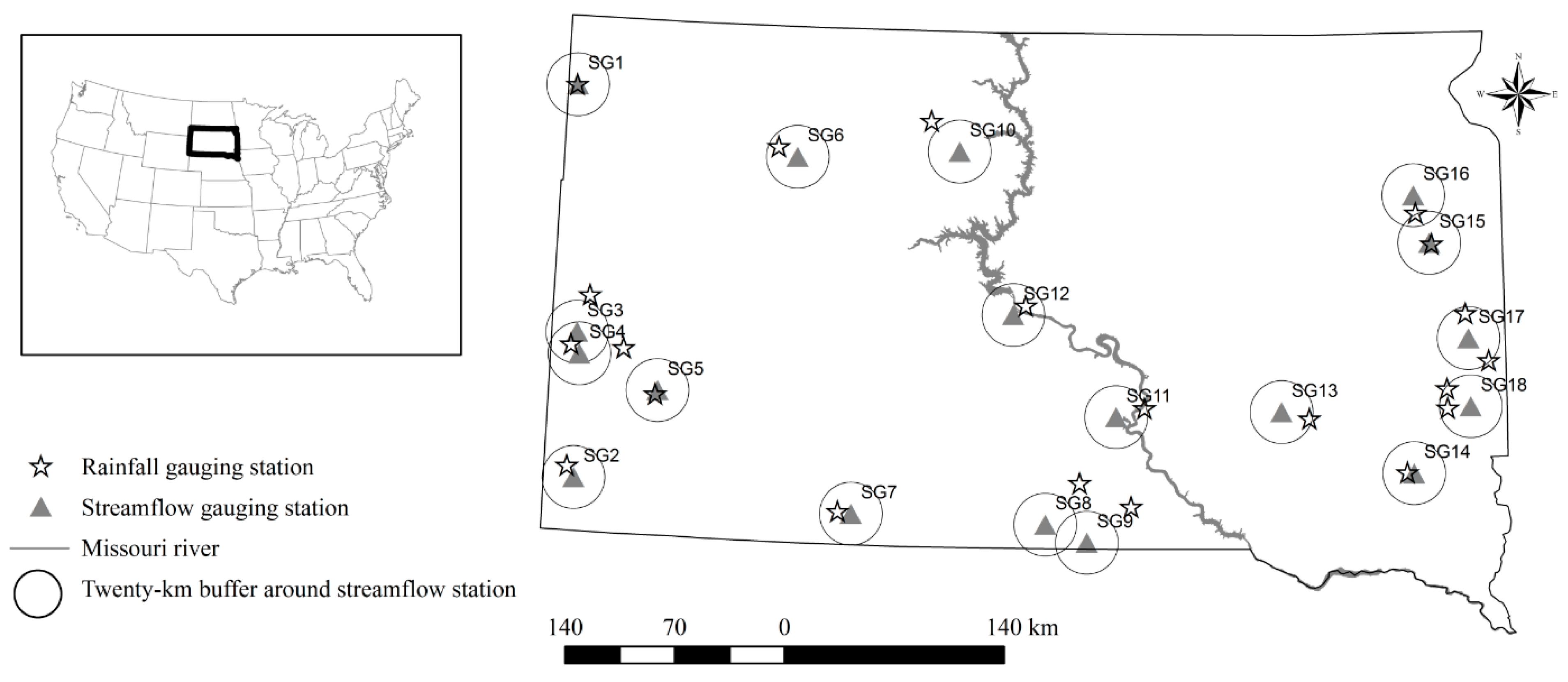
3. Data Used
- The station must have at least 30 years of continuous streamflow data.
- The station must be free from diversion and regulation.

| USGS Streamflow Station Name | USGS Station Number | Notation | Start Year | Data Length (Years) | Drainage Area (km2) |
|---|---|---|---|---|---|
| Bad River near Fort Pierre, SD | 06441500 | SG12 | 1951 | 63 | 8151 |
| Battle Creek at Hermosa, SD | 06406000 | SG5 | 1951 | 63 | 438 |
| Big Sioux River near Brookings, SD | 06480000 | SG17 | 1963 | 51 | 8645 |
| Big Sioux River near Castlewood, SD | 06479525 | SG15 | 1977 | 37 | 2836 |
| Big Sioux River near Dell Rapids, SD | 06481000 | SG18 | 1951 | 63 | 10,168 |
| Big Sioux River near Watertown, SD | 06479438 | SG16 | 1977 | 37 | 1360 |
| Castle Creek near Deerfield Res and Hill City, SD | 06409000 | SG4 | 1951 | 63 | 205 |
| Cheyenne River at Edgemont, SD | 06395000 | SG2 | 1951 | 63 | 18,658 |
| Firesteel Creek near West Vernon, SD | 06477500 | SG13 | 1963 | 51 | 1520 |
| Keya Paha River near Keya Paha, SD | 06464100 | SG8 | 1982 | 32 | 1386 |
| Keya Paha River at Wewela, SD | 06464500 | SG9 | 1951 | 63 | 2924 |
| Little Missouri River at Camp Crook, SD | 06334500 | SG1 | 1963 | 51 | 5112 |
| Little White River near Martin, SD | 06447500 | SG7 | 1963 | 51 | 811 |
| Moreau River near Faith, SD | 06359500 | SG6 | 1951 | 63 | 6723 |
| Moreau River near Whitehorse, SD | 06360500 | SG10 | 1963 | 51 | 12,675 |
| Rhoads Fork near Rochford, SD | 06408700 | SG3 | 1982 | 32 | 20 |
| West Fork Vermillion River near Parker, SD | 06478690 | SG14 | 1963 | 51 | 979 |
| White River near Oacoma, SD | 06452000 | SG11 | 1951 | 63 | 25,693 |
| Rainfall station name | Network ID | Data length (years) | |||
| Brookings 2 NE, SD | GHCND: USC00391076 | 51 | |||
| Camp Crook, SD | GHCND: USC00391294 | 51 | |||
| Castlewood, SD | GHCND: USC00391519 | 51 | |||
| Chamberlin 5S | GHCND: USC00391609 | 63 | |||
| Chester, SD | GHCND: USC00391634 | 63 | |||
| Colton, SD | GHCND: USC00391851 | 63 | |||
| Deerfield 4 NW, SD | GHCND: USC00392228 | 63 | |||
| Edgemont, SD | GHCND: USC00392557 | 63 | |||
| Flandreau, SD | GHCND: USC00392984 | 63 | |||
| Gregory, SD | GHCND: USC00393452 | 63 | |||
| Hermosa 3 SSW, SD | GHCND: USC00393775 | 51 | |||
| Lead, SD | GHCND: USC00394834 | 32 | |||
| Marion, SD | GHCND: USC00395228 | 51 | |||
| Martin, SD | GHCND: USC00395281 | 51 | |||
| Mitchell 2 N, SD | GHCND: USC00395671 | 51 | |||
| Pactola Dam, SD | GHCND: USC00396427 | 32 | |||
| Pierre Regional Airport, SD | GHCND:USW00024025 | 63 | |||
| Timber Lake, SD | GHCND: USC00398307 | 63 | |||
| Usta 8 WNW Kelly Ranch, SD | GHCND: USC00398528 | 63 | |||
| Watertown Regional Airport, SD | GHCND: USW00014946 | 51 | |||
| Winner, SD | GHCND: USC00399367 | 32 | |||
4. Methodology
4.1. Computation of Streamflow, Rainfall, and Land Use Statistics
4.2. Trend Analysis
4.3. Streamflow Elasticity Analysis
5. Results and Discussion
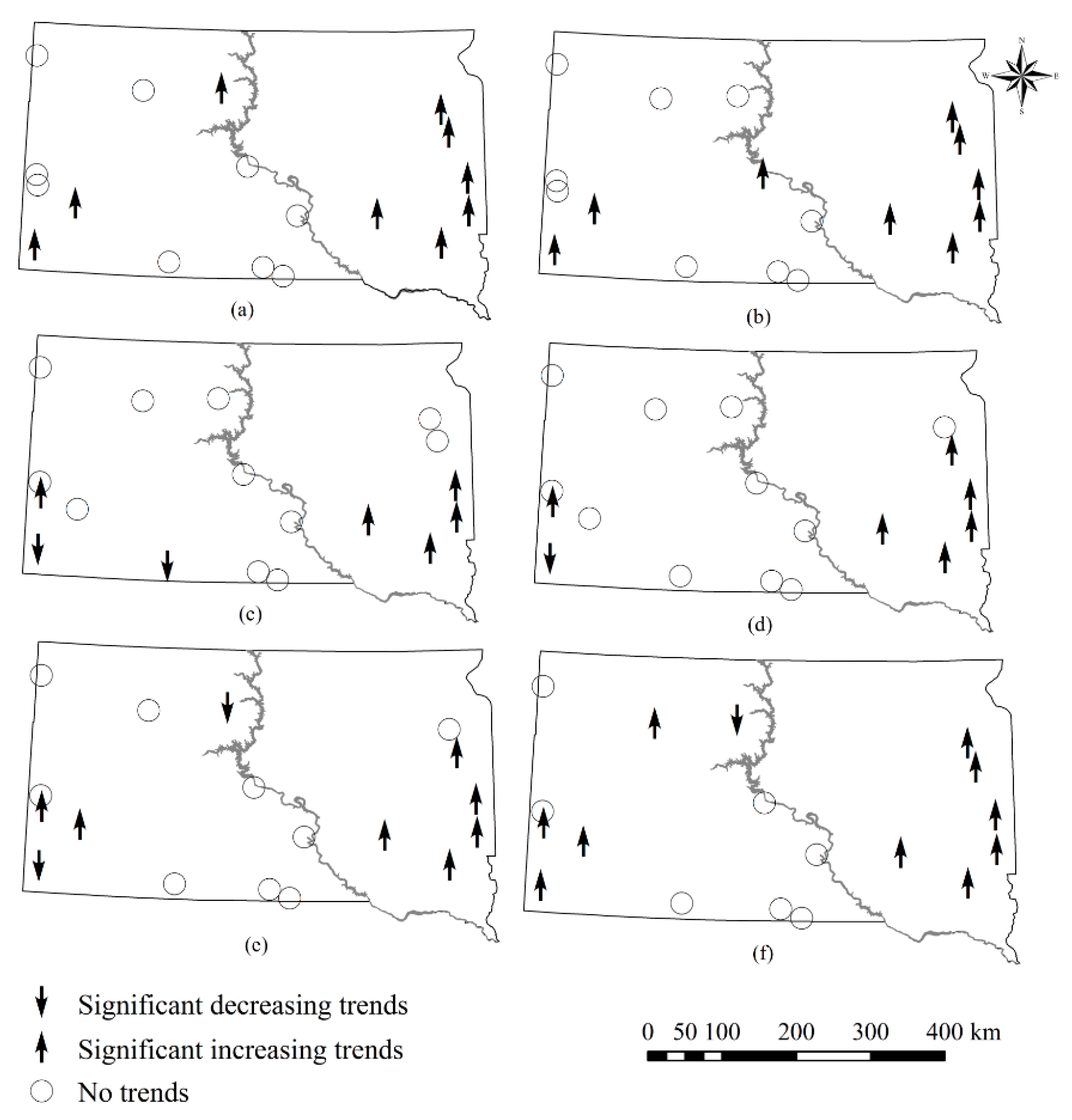
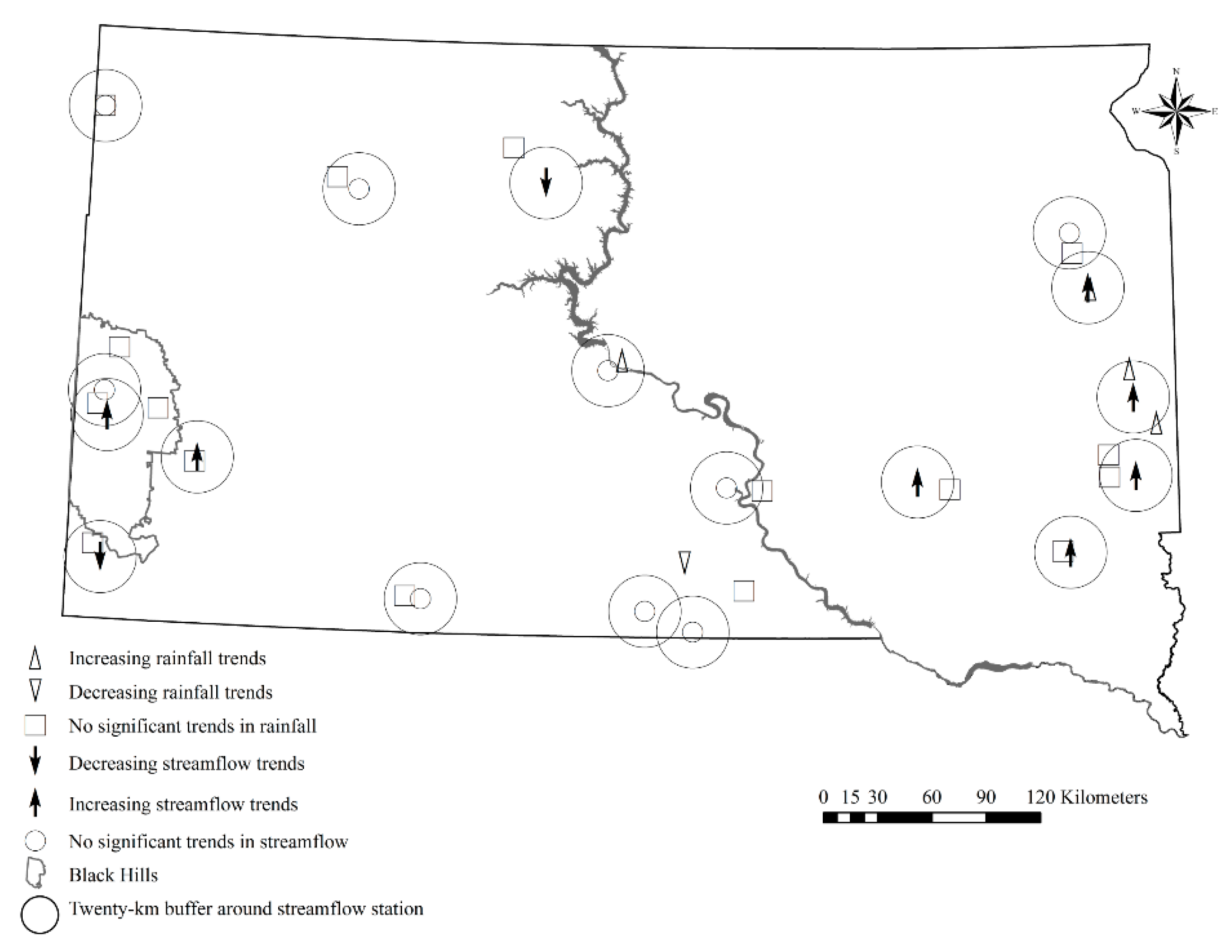
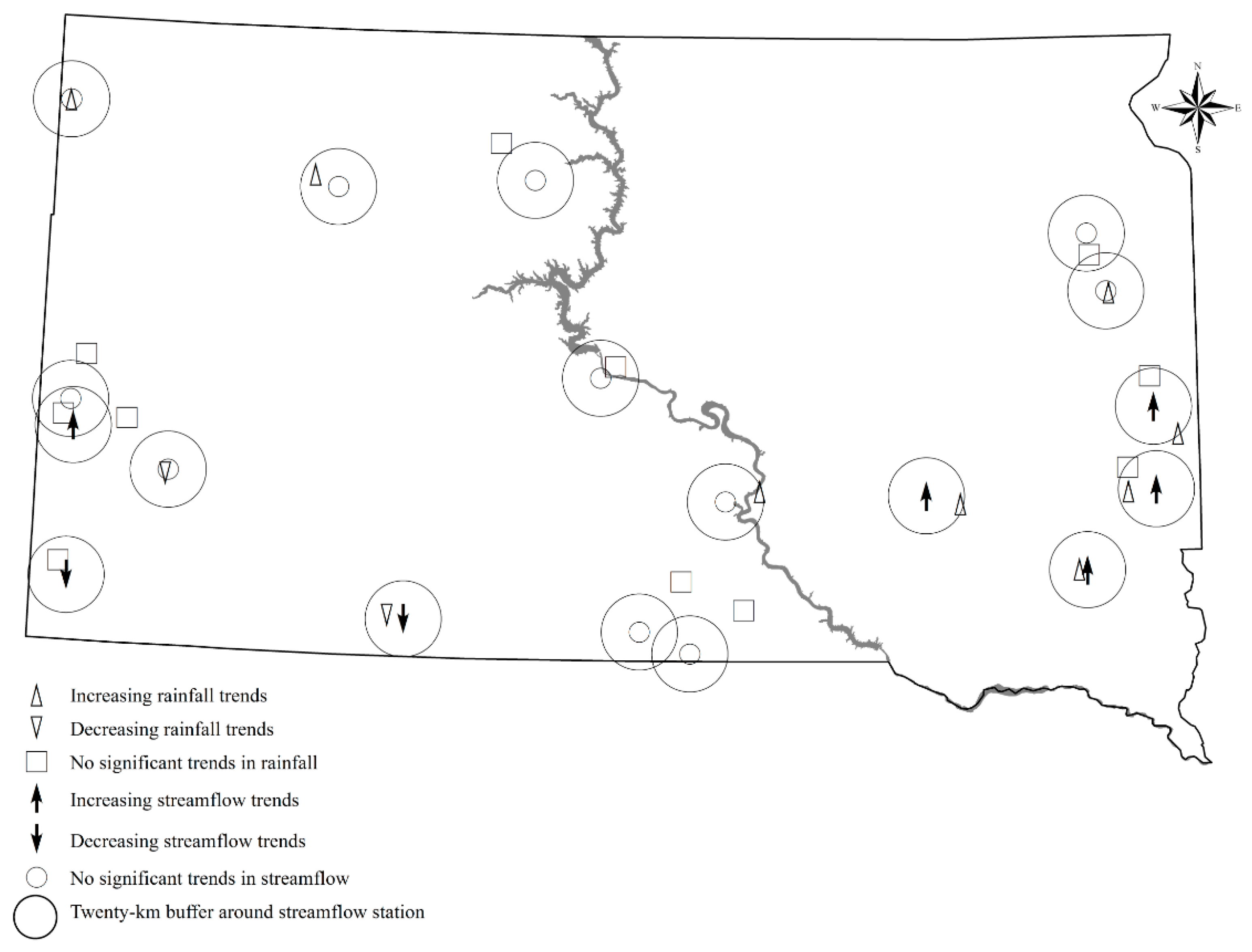
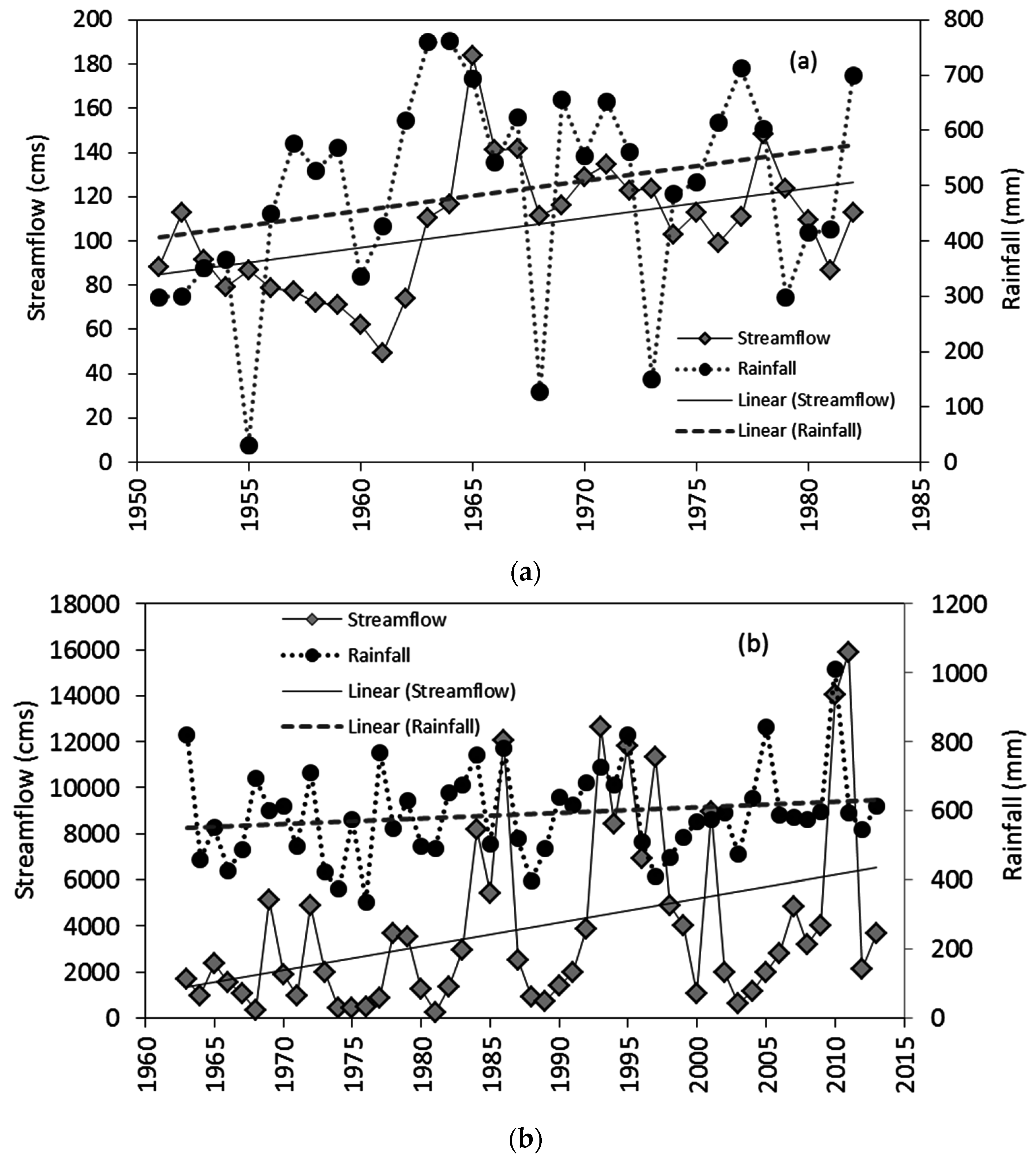
5.1. Trends in Streamflow and Rainfall
| USGS Station Number | Annual Streamflow | One-Day Min (Low Flow) | Seven-Day Min (Low Flow) | One-Day Max (High Flow) | Seven-Day Max (High Flow) | Median Daily (Flow) | Daily Average (Flow) |
|---|---|---|---|---|---|---|---|
| 06359500 | 1.2 (0.20)[0.09] | 1.5(0.12) | 1.6(0.11) | 0.8(0.42) | 0.9(0.32) | 1.7 (0.08) | 1.3 (0.20) |
| 06395000 | −2.1(0.04)[−0.03] | 2.4(0.01) | 2.3(0.01) | −2.7(0.01) | −2.2(0.02) | 1.8(0.07) | −2.0(0.04) |
| 06409000 | 1.8(0.08)[0.41] | 1.5(0.12) | 1.6(0.11) | 1.9(0.05) | 1.6(0.09) | 1.8(0.07) | 1.8(0.08) |
| 06441500 | −0.5(0.62)[−0.03] | 1.1(0.25) | 1.9(0.05) | −0.9(0.33) | 0.1(0.91) | −0.5(0.64) | −0.5(0.62) |
| 06452000 | 0.9(0.35)[0.08] | 1.1(0.26) | 1.0(0.29) | 0.6(0.54) | 0.1(0.97) | 1.5(0.13) | 0.9(0.35) |
| 06464500 | 0.9(0.39)[0.11] | 1.0(0.30) | 1.1(0.26) | 0.5(0.57) | 1.1(0.27) | 1.3(0.18) | 0.9(0.39) |
| 06481000 | 1.8(0.08)[0.53] | 2.2(0.02) | 2.2(0.02) | 3.2(<0.10) | 2.9(<0.10) | 2.1(0.03) | 1.8(0.08) |
| 06406000 | 1.7(0.09)[0.23] | 2.5(0.01) | 2.4(0.01) | −0.1(0.93) | 0.9(0.35) | 2.0(0.04) | 1.7(0.095) |
| 06360500 | −3.9((<0.10)[−0.21] | 1.8(0.07) | 1.6 (0.11) | 0.4(0.66) | 0.1(0.91) | −2.5(0.01) | −3.9 (<0.10) |
| 06477500 | 1.8(0.07)[0.23] | 2.5(0.01) | 2.8(<0.10) | 2.2(0.03) | 2.0(0.04) | 2.2(0.03) | 1.8(0.07) |
| 06478690 | 2.5(0.01)[0.68] | 3.3(<0.10) | 3.4(<0.10) | 2.2(0.02) | 2.4(0.02) | 2.6(0.01) | 2.6(0.01) |
| 06334500 | −0.3(0.73)[−0.4] | 1.4(0.16) | 1.5(0.12) | −0.6(0.52) | −0.4(0.72) | −0.7(0.51) | −0.3(0.73) |
| 06447500 | 0.7(0.46)[0.07] | 1.4(0.16) | 1.2(0.20) | −2.0(0.04) | −1.6(0.12) | 1.1(0.29) | 0.7(0.46) |
| 06480000 | 1.9(0.05)[0.60] | 2.5(0.01) | 2.4(0.01) | 2.4(0.02) | 2.6(0.01) | 2.4(0.02) | 1.9(0.05) |
| 06479525 | 1.8(0.07)[0.03] | 2.4(0.02) | 2.2(0.02) | 0.9(0.35) | 1.9(0.05) | 2.1(0.03) | 1.8(0.07) |
| 06479438 | 1.5(0.13)[0.41] | 2.1(0.03) | 1.9(0.06) | 1.1(0.29) | 0.9(0.37) | 2.1(0.03) | 1.5(0.13) |
| 06408700 | 0.2(0.82)[0.46] | 0.2(0.82) | 0.3(0.73) | 0.2(0.85) | 0.001(1.00) | 0.2(0.81) | 0.2(0.85) |
| 06464100 | 0.1(0.86)[0.02] | 0.6(0.54) | 0.8(0.42) | 0.3(0.75) | 0.5(0.60) | 0.3(0.77) | 0.2(0.86) |
| USGS Station Number | Fall | Spring | Summer | Winter |
|---|---|---|---|---|
| 06359500 | 2.67(0.01)[0.004] | 1.27(0.20)[[0.015] | 0.17(0.86)[[0.001] | 2.60(0.01)[0.006] |
| 06395000 | 1.72(0.09)[0.001] | 1.38(0.17)[[0.002] | −1.99(0.05)[−0.008] | 2.17(0.03)[0.002] |
| 06409000 | 0.48(0.63)[[0.002] | 0.91(0.36)[[0.003] | 0.92(0.36)[[0.0025] | 0.26(0.79)[[0.001] |
| 06441500 | 0.32(0.75)[[0.0001] | −0.50(0.62)[−0.004] | −0.97(0.33)[−0.007] | 0.82(0.41)[[0.001] |
| 06452000 | 1.69(0.09)[0.011] | 0.84(0.39)[[0.016] | 0.50(0.62)[[0.006] | 1.94(0.05)[0.013] |
| 06464500 | 1.35(0.18)[[0.013] | 0.94(0.35)[[0.021] | 1.69(0.09)[0.026] | 1.48(0.14)[[0.023] |
| 06481000 | 2.32(0.02)[0.055] | 1.72(0.08)[0.172] | 1.76(0.08)[0.106] | 2.09(0.04)[0.007] |
| 06406000 | 2.00(0.05)[0.056] | 1.58(0.11)[[0.048] | 1.50(0.13)[[0.037] | 2.48(0.01)[0.047] |
| 06360500 | −5.33(<0.10)[−0.002] | −4.41(<0.10)[−0.066] | −3.46(<0.10)[−0.027] | −2.42(0.02)[−0.001] |
| 06477500 | 2.55(0.01)[0.001] | 1.44(0.15)[[0.021] | 2.68(0.01)[0.049] | 3.10(<0.10)[0.002] |
| 06478690 | 2.94(<0.10)[0.007] | 2.06(0.04)[0.110] | 3.54(<0.10)[0.087] | 2.86(<0.10)[0.009] |
| 06334500 | 0.39(0.69)[[0.0013] | −0.46(0.64)[−0.015] | −1.12(0.26)[−0.017] | 0.70(0.48)[[0.001] |
| 06447500 | 1.25(0.21)[[0.008] | 1.11(0.27)[[0.023] | 0.14(0.89)[[0.003] | 1.97(0.05)[0.027] |
| 06480000 | 2.41(0.02)[0.065] | 1.79(0.07)[0.209] | 1.91(0.06)[0.12] | 2.23(0.03)[0.039] |
| 06479525 | 2.17(0.03)0.043] | 1.92(0.05)[0.171] | 1.79(0.07)[0.064] | 2.16(0.03)[0.025] |
| 06479438 | 2.24(0.02)0.036] | 1.55(0.12)[[0.139] | 1.24(0.21)[[0.035] | 2.03(0.04)[0.017] |
| 06408700 | −0.01(0.99)[−0.01] | 0.33(0.74)[[0.134] | 0.23(0.82)[[0.059] | 0.36(0.72)[[0.164] |
| 06464100 | −0.21(0.83)[ −0.002] | 0.34(0.73)[[0.022] | −0.11(0.91)[−0.003] | 0.62(0.53)[[0.016] |


| Rainfall Gauging Station Number | Annual Rainfall | One-Day Maximum Rainfall |
|---|---|---|
| GHCND: USC00398528 | −1.13(0.26)[−2.35] | 1.64(0.09) |
| GHCND: USC00392557 | −0.74(0.46)[−0.59] | 0.53(0.59) |
| GHCND: USC00392228 | 0.00(0.99)[4.02] | 0.84(0.40) |
| GHCND:USW00024025 | 1.73(0.08)[0.94] | 0.09(0.92) |
| GHCND: USC00391609 | 0.71(0.48)[1.48] | 1.76(0.08) |
| GHCND: USC00393452 | 1.55(0.12)[1.85] | 1.54(0.12) |
| GHCND: USC00391851 | −1.53(0.12)[−4.56] | 2.02(0.04) |
| GHCND: USC00391634 | −0.69(0.49)[−3.50] | 0.61(0.54) |
| GHCND: USC00393775 | 1.17(0.24)[1.53] | −2.12(0.03) |
| GHCND: USC00398307 | 0.94(0.35)[0.64] | −0.96(0.34) |
| GHCND: USC00395671 | 1.30(0.19)[1.63] | 1.79(0.07) |
| GHCND: USC00395228 | 0.52(0.60)[0.58] | 1.71(0.08) |
| GHCND: USC00391294 | 1.04(0.30)[1.15] | 1.62(0.09) |
| GHCND: USC00395281 | 1.24(0.21)[1.68] | −4.26(<0.10) |
| GHCND: USC00391076 | 1.63(0.10)[1.25] | 1.43(0.15) |
| GHCND: USC00392984 | 1.74(0.08)[2.61] | 2.16(0.03) |
| GHCND: USC00391519 | 2.01(0.04)[1.55] | 2.00(0.04) |
| GHCND: USW00014946 | −0.25(0.80)[−0.38] | 0.91(0.36) |
| GHCND: USC00396427 | −0.64(0.52)[−0.83] | 1.47(0.14) |
| GHCND: USC00394834 | 1.55(0.12)[4.48] | 1.07(0.28) |
| GHCND: USC00399367 | −1.74(0.08)[−3.62] | −0.87(0.38) |
| Rainfall Station | Fall | Spring | Summer | Winter |
|---|---|---|---|---|
| GHCND: USC00398528 | −0.58 (0.56)[−0.16] | −1.57(0.11)[−0.81] | −1.08(0.28)[−0.59] | −2.16(0.03)[−0.31] |
| GHCND: USC00392557 | −0.045(0.96)[−0.02] | 0.14(0.89)[0.06] | −2.00(0.05)[−0.94] | 0.48(0.63)[0.12] |
| GHCND: USC00392228 | 0(1.00)[−0.12] | −0.25(0.80)[−0.30] | 0.80(0.42)[0.81] | 2.42(0.02)[1.49] |
| GHCND:USW00024025 | 0(1.00)[0.87] | 1.64(0.09)[0.28] | −0.42(0.67)[−0.14] | −0.54(0.59)[−0.11] |
| GHCND: USC00391609 | −0.08(0.934)[−0.8] | −1.53(0.13)[−0.91] | 1.06(0.29)[0.87) | 1.79(0.07)[0.38] |
| GHCND: USC00393452 | 1.34(0.18)[1.57] | −1.31(0.19)[−1.62] | 1.76(0.08)[1.90] | 0.62(0.54)[0.22] |
| GHCND: USC00391851 | −1.21(0.23)[−0.8] | −1.15(0.25)[−1.14] | −1.55(0.12)[−2.52] | 0.02(0.98)[0.02] |
| GHCND: USC00391634 | −0.693(0.49)[−1.53] | 0.00(1.00)[−0.04] | −0.52(0.60)[−0.76] | −1.40(0.16)[−1.26] |
| GHCND: USC00393775 | 1.392(0.16)[0.46] | 1.19(0.23)[1.73] | 0.24(0.81)[1.73] | −0.21(0.83)[−0.02] |
| GHCND: USC00398307 | 1.493(0.14)[0.47] | −0.65(0.52)[−0.26] | 0.21(0.83)[0.07] | 1.89(0.06)[0.22] |
| GHCND: USC00395671 | 1.79(0.07)[1.18] | 1.15(0.25)[0.64] | −1.60(0.11)[−0.70] | 1.13(0.26)[0.14] |
| GHCND: USC00395228 | −1.168(0.24)[−0.31] | 1.48(0.14)[0.64] | 0.00(1.00)[−0.01] | 0.17(0.86)[0.05] |
| GHCND: USC00391294 | 1.33(0.18)[0.08] | 1.28(0.20)[0.08] | 0.46(0.64)[0.22] | 0.61(0.54)[0.07] |
| GHCND: USC00395281 | 2.02 (0.02)[0.85] | 0.47(0.64)[0.23] | −0.25(0.80)[−0.36] | 1.86(0.06)[0.30] |
| GHCND: USC00391076 | 1.19(0.23)[0.79] | 1.84(0.07)[0.73] | 0.04(0.96)[0.01] | 1.31(0.19)[0.27] |
| GHCND: USC00392984 | 2.18(0.03)[1.40] | 1.36(0.17)[0.61] | 1.07(0.29)[0.58] | 0.21(0.83)[0.05] |
| GHCND: USC00391519 | 1.85(0.06)[0.88] | 0.77(0.44)[0.16] | 0.12(0.90)[0.03] | −0.98(0.33)[−0.07] |
| GHCND: USW00014946 | 2.92(<0.10)[0.86] | −0.49(0.63)[−0.23] | −1.28(0.20)[−0.48] | 0.28(0.78)[0.08] |
| GHCND: USC00396427 | −1.66(0.09)[−0.84] | 1.33(0.18)[1.19] | −1.22(0.22)[−1.15] | 1.03(0.30)[0.16] |
| GHCND: USC00394834 | 0.709(0.48)[0.50] | 0.49(0.62)[0.75] | 0.79(0.43)[0.76] | 1.89(0.06)[1.74] |
| GHCND: USC00399367 | −1.544(0.12)[−1.13] | −1.59(0.11)[−1.64] | −1.64(0.09)[−2.36] | 0.95(0.34)[−0.31] |

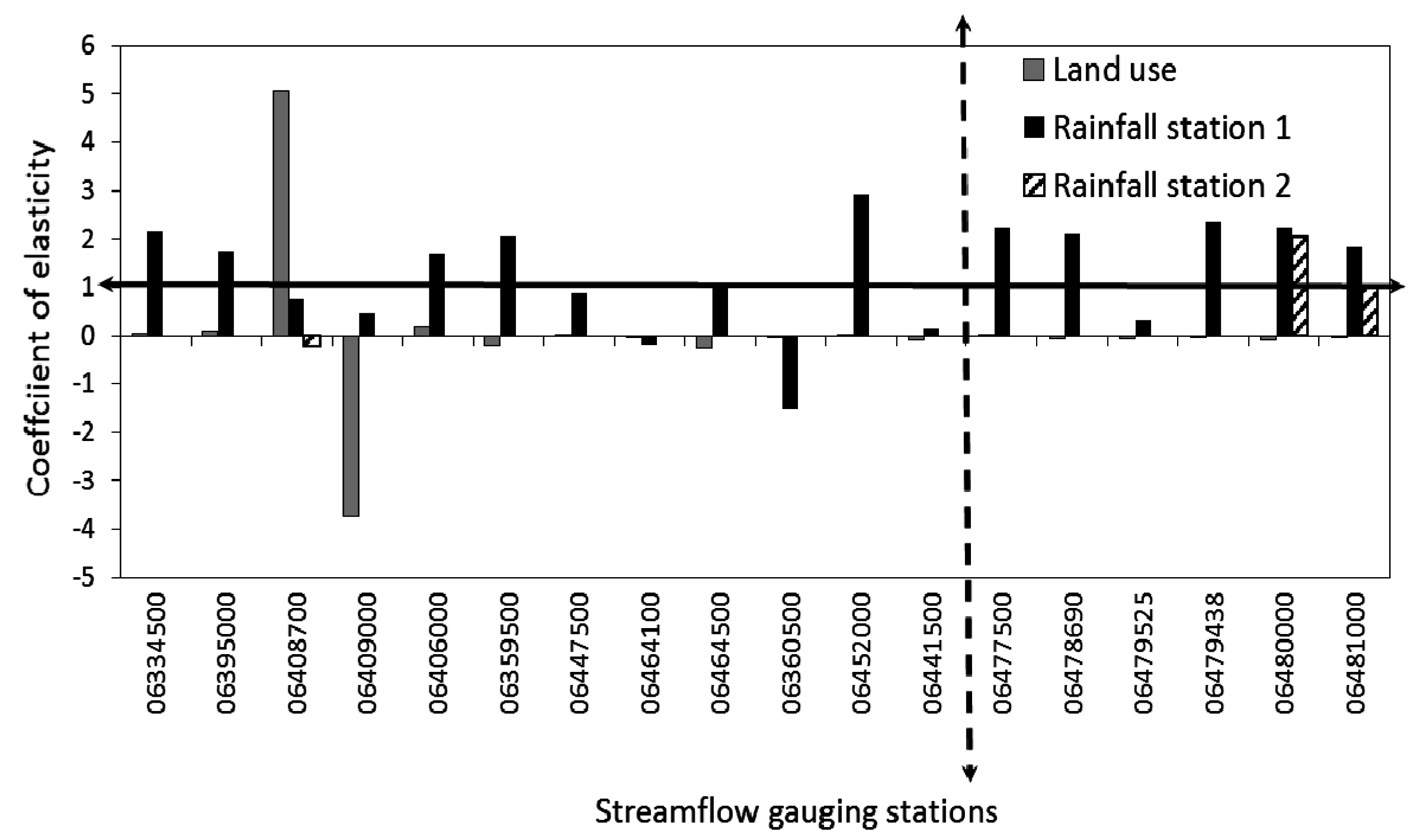
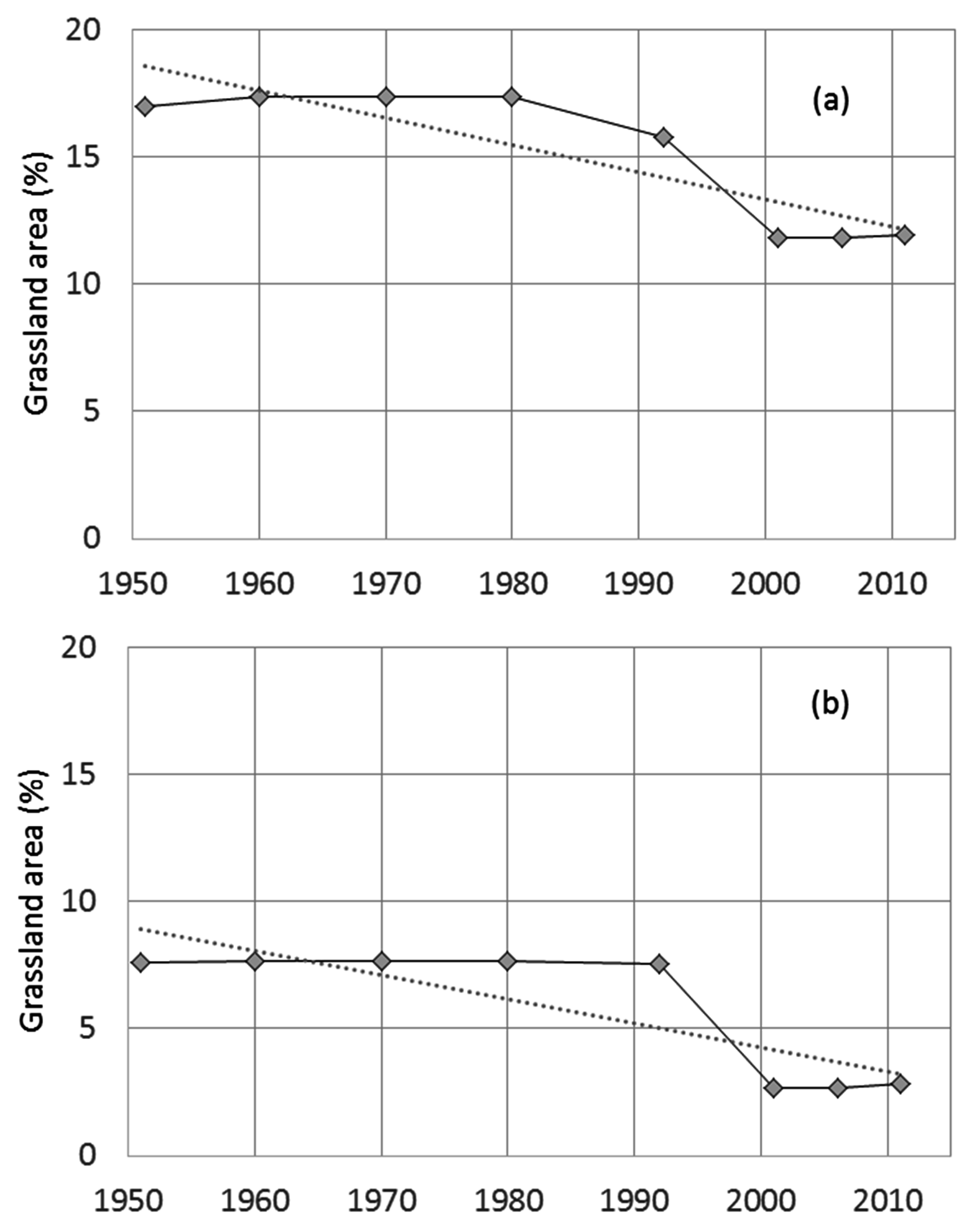
5.2. Elasticity of Streamflow to Rainfall and Change in Grassland Area

6. Conclusions
Acknowledgments
Author Contributions
Conflicts of Interest
References
- Samson, F.B.; Knopf, F.L.; Ostlie, W.R. Great plains ecosystems: Past, present, and future. Wildl. Soc. Bull. 2004, 32, 6–15. [Google Scholar] [CrossRef]
- Reitsma, K.D.; Dunn, B.H.; Smart, A.J.; Clay, S.A.; Carlson, C.G. Estimated South Dakota Land Use Change from 2006 to 2012; SDSU Department of Plant Science, SDSU Extension: Brookings, SD, USA, 2013. [Google Scholar]
- Wright, C.K.; Wimberly, M.C. Recent land use change in the western corn belt threatens grasslands and wetlands. Proc. Natl. Acad. Sci. USA. 2013, 110, 4134–4139. [Google Scholar] [CrossRef] [PubMed]
- Rosentrater, K.A.; Todey, D.; Persyn, R. Quantifying total and sustainable agricultural biomass resources in South Dakota—A preliminary assessment. Agric. Eng. Int. 2009, 11, 1–14. [Google Scholar]
- Olson, A.L.; Klein, N.; Taylor, G. The Impact of Increased Ethanol Production on Corn Basis in South Dakota. Ph.D. Thesis, South Dakota State University, Brookings, SD, USA, 2007. [Google Scholar]
- Schmer, M.R.; Dose, H.L. Cob biomass supply for combined heat and power and biofuel in the north central USA. Biomass Bioenergy 2014, 64, 321–328. [Google Scholar] [CrossRef]
- United States Congress—Senate. Energy Independence and Security Act of 2007. HR 6. 110th Congress, 1st Session. Available online: https://www.govtrack.us/congress/bills/110/hr2304 (accessed on 23 December 2015).
- Altieri, M.A. The ecological impacts of large-scale agrofuel monoculture production systems in the americas. Bull. Sci. Technol. Soc. 2009, 29, 236–244. [Google Scholar] [CrossRef]
- Lüscher, A. Land use systems in grassland dominated regions. In Proceedings of the 20th general meeting of the European grassland federation, Luzern, Switzerland, 21–24 June 2004.
- Boval, M.; Dixon, R. The importance of grasslands for animal production and other functions: A review on management and methodological progress in the tropics. Animal 2012, 6, 748–762. [Google Scholar] [CrossRef] [PubMed]
- Carlier, L.; Rotar, I.; Vlahova, M.; Vidican, R. Importance and functions of grasslands. Not. Bot. Horti Agrobot. 2009, 37, 25–30. [Google Scholar]
- Claassen, R.; Carriazo, F.; Cooper, J.C.; Hellerstein, D.; Ueda, K. Grassland to Cropland Conversion in the Northern Plains: The Role of Crop Insurance, Commodity, and Disaster Programs; Economic Research Service, U.S Department of Agriculture: Washington DC, USA, 2011.
- Schilling, K.E.; Chan, K.-S.; Liu, H.; Zhang, Y.-K. Quantifying the effect of land use land cover change on increasing discharge in the Upper Mississippi River. J. Hydrol. 2010, 387, 343–345. [Google Scholar] [CrossRef]
- Zhang, Y.-K.; Schilling, K. Increasing streamflow and baseflow in Mississippi River since the 1940s: Effect of land use change. J. Hydrol. 2006, 324, 412–422. [Google Scholar] [CrossRef]
- Schilling, K.E.; Jha, M.K.; Zhang, Y.K.; Gassman, P.W.; Wolter, C.F. Impact of land use and land cover change on the water balance of a large agricultural watershed: Historical effects and future directions. Water Resour. Res. 2008. [Google Scholar] [CrossRef]
- Huntington, T.G. Evidence for intensification of the global water cycle: Review and synthesis. J. Hydrol. 2006, 319, 83–95. [Google Scholar] [CrossRef]
- Tan, M.L.; Ibrahim, A.L.; Yusop, Z.; Duan, Z.; Ling, L. Impacts of land-use and climate variability on hydrological components in the Johor river basin, Malaysia. Hydrol. Sci. J. 2015, 60, 873–889. [Google Scholar] [CrossRef]
- Wei, X.; Liu, W.; Zhou, P. Quantifying the relative contributions of forest change and climatic variability to hydrology in large watersheds: A critical review of research methods. Water 2013, 5, 728–746. [Google Scholar] [CrossRef]
- Xu, X.; Scanlon, B.R.; Schilling, K.; Sun, A. Relative importance of climate and land surface changes on hydrologic changes in the US Midwest since the 1930s: Implications for biofuel production. J. Hydrol. 2013, 497, 110–120. [Google Scholar] [CrossRef]
- Nejadhashemi, A.; Wardynski, B.; Munoz, J. Evaluating the impacts of land use changes on hydrologic responses in the agricultural regions of Michigan and Wisconsin. Hydrol. Earth Syst. Sci. Discuss. 2011, 8, 3421–3468. [Google Scholar] [CrossRef]
- Fitzpatrick, F.A.; Knox, J.C.; Whitman, H.E. Effects of Historical Land-Cover Changes on Flooding and Sedimentation, North Fish Creek, Wisconsin; US Department of the Interior, US Geological Survey: Middleton, WI, USA, 1999.
- Frans, C.; Istanbulluoglu, E.; Mishra, V.; Munoz-Arriola, F.; Lettenmaier, D.P. Are climatic or land cover changes the dominant cause of runoff trends in the Upper Mississippi River Basin? Geophys. Res. Lett. 2013, 40, 1104–1110. [Google Scholar] [CrossRef]
- Hu, Z.; Wang, L.; Wang, Z.; Hong, Y.; Zheng, H. Quantitative assessment of climate and human impacts on surface water resources in a typical semi-arid watershed in the middle reaches of the Yellow River from 1985 to 2006. Int. J. Climatol. 2015, 35, 97–113. [Google Scholar] [CrossRef]
- Kim, J.; Choi, J.; Choi, C.; Park, S. Impacts of changes in climate and land use/land cover under ipcc rcp scenarios on streamflow in the Hoeya River Basin, Korea. Sci. Total Environ. 2013, 452, 181–195. [Google Scholar] [CrossRef] [PubMed]
- Kumar, S.; Merwade, V.; Kam, J.; Thurner, K. Streamflow trends in Indiana: Effects of long term persistence, precipitation and subsurface drains. J. Hydrol. 2009, 374, 171–183. [Google Scholar] [CrossRef]
- Novotny, E.V.; Stefan, H.G. Stream flow in Minnesota: Indicator of climate change. J. Hydrol. 2007, 334, 319–333. [Google Scholar] [CrossRef]
- Vogel, R.M. Hydromorphology. J. Water Resour. Plan. Manag. 2011, 137, 147–149. [Google Scholar] [CrossRef]
- Wang, D.; Hejazi, M. Quantifying the relative contribution of the climate and direct human impacts on mean annual streamflow in the contiguous United States. Water Resour. Res. 2011. [Google Scholar] [CrossRef]
- Yang, Z.F.; Yan, Y.; Liu, Q. The relationship of streamflow-precipitation-temperature in the Yellow River Basin of China during 1961–2000. Procedia Environ. Sci. 2012, 13, 2336–2345. [Google Scholar] [CrossRef]
- Adam, J.C.; Hamlet, A.F.; Lettenmaier, D.P. Implications of global climate change for snowmelt hydrology in the twenty-first century. Hydrol. Process. 2009, 23, 962–972. [Google Scholar] [CrossRef]
- Barnett, T.P.; Pierce, D.W.; Hidalgo, H.G.; Bonfils, C.; Santer, B.D.; Das, T.; Bala, G.; Wood, A.W.; Nozawa, T.; Mirin, A.A. Human-induced changes in the hydrology of the western United States. Science 2008, 319, 1080–1083. [Google Scholar] [CrossRef] [PubMed]
- Brabets, T.P.; Walvoord, M.A. Trends in streamflow in the Yukon River Basin from 1944 to 2005 and the influence of the pacific decadal oscillation. J. Hydrol. 2009, 371, 108–119. [Google Scholar] [CrossRef]
- Jones, J.A. Hydrologic responses to climate change: Considering geographic context and alternative hypotheses. Hydrol. Process. 2011, 25, 1996–2000. [Google Scholar] [CrossRef]
- Wilson, D.; Hisdal, H.; Lawrence, D. Has streamflow changed in the nordic countries?—Recent trends and comparisons to hydrological projections. J. Hydrol. 2010, 394, 334–346. [Google Scholar] [CrossRef]
- Xu, C.; Chen, Y.; Hamid, Y.; Tashpolat, T.; Chen, Y.; Ge, H.; Li, W. Long-term change of seasonal snow cover and its effects on river runoff in the Tarim River Basin, northwestern China. Hydrol. Process. 2009, 23, 2045–2055. [Google Scholar] [CrossRef]
- Guo, H.; Hu, Q.; Jiang, T. Annual and seasonal streamflow responses to climate and land-cover changes in the Poyang Lake Basin, China. J. Hydrol. 2008, 355, 106–122. [Google Scholar] [CrossRef]
- Sagarika, S.; Kalra, A.; Ahmad, S. Evaluating the effect of persistence on long-term trends and analyzing step changes in streamflows of the continental United States. J. Hydrol. 2014, 517, 36–53. [Google Scholar] [CrossRef]
- Tohver, I.M.; Hamlet, A.F.; Lee, S.Y. Impacts of 21st-century climate change on hydrologic extremes in the pacific northwest region of north America. J. Am. Water Resour. Assoc. 2014, 50, 1461–1476. [Google Scholar] [CrossRef]
- Lins, H.F.; Slack, J.R. Streamflow trends in the United States. Geophys. Res. Lett. 1999, 26, 227–230. [Google Scholar] [CrossRef]
- Norton, P.A.; Anderson, M.T.; Stamm, J.F. Trends in Annual, Seasonal, and Monthly Streamflow Characteristics at 227 Streamgages in the Missouri River Watershed, Water Years 1960–2011; US Geological Survey: Reston, VA, USA, 2014.
- United States Department of Agriculture. Summary Report: 1997 National Resources Inventory (Revised December 2000). Available online: http://www.nrcs.usda.gov/Internet/FSE_DOCUMENTS/nrcs143_012094.pdf (accessed on 23 December 2015).
- South Dakota Department of Agriculture, Ecosystem Research Group. Draft Coordinated Plan for Natural Resources Conservation; South Dakota Department of Agriculture: Pierre, South Dakota, USA, 2006.
- South Dakota Department of Agriculture and HDR Engineering Inc. South Dakota Coordinated Plan for Natural Resources Conservation; State Conservation Commission: Pierre, SD, USA, 2012.
- National Agricultural Statistics Service. Quickstats. Available online: http://quickstats.nass.usda.gov/ (accessed on 1 July 2015).
- South Dakota Office of Climatology. South Dakota Climate and Weather. Available online: http://climate.sdstate.edu/climate_site/climate.htm (accessed on 1 July 2015).
- Saad, D.A.; Schwarz, G.E.; Robertson, D.M.; Booth, N.L. A multi-agency nutrient dataset used to estimate loads, improve monitoring design, and calibrate regional nutrient sparrow models1. J. Am. Water Resour. Assoc. 2011, 47, 933–949. [Google Scholar] [CrossRef] [PubMed][Green Version]
- Ahiablame, L.; Engel, B.; Chaubey, I. An optimization method for estimating constituent mean concentrations in base flow-dominated flow. J. Am. Water Resour. Assoc. 2013, 49, 1167–1178. [Google Scholar] [CrossRef]
- The Nature Conservancy. Indicators of Hydrologic Alteration Version 7.1: User’s Manual; The Nature Conservancy: Arlington, VA, USA, 2009. [Google Scholar]
- Hamed, K.H.; Rao, A.R. A modified Mann-Kendall trend test for autocorrelated data. J. Hydrol. 1998, 204, 182–196. [Google Scholar] [CrossRef]
- Durbin, J.; Watson, G.S. Testing for serial correlation in least squares regression. I. Biometrika 1950, 37, 409–428. [Google Scholar] [PubMed]
- Savin, N.E.; White, K.J. The Durbin-Watson test for serial correlation with extreme sample sizes or many regressors. Econom. J. Econom. Soc. 1977, 45, 1989–1996. [Google Scholar] [CrossRef]
- Hirsch, R.M.; Slack, J.R. A Non-parametric trend test for seasonal data with serial dependence. Water Resour. Res. 1984, 20, 727–732. [Google Scholar] [CrossRef]
- Yue, S.; Pilon, P.; Phinney, B.; Cavadias, G. The influence of autocorrelation on the ability to detect trend in hydrological series. Hydrol. Process. 2002, 16, 1807–1829. [Google Scholar] [CrossRef]
- Mann, H.B. Nonparametric tests against trend. Econom. J. Econom. Soc. 1945, 13, 245–259. [Google Scholar] [CrossRef]
- Zhang, X.; Zhang, L.; Zhao, J.; Rustomji, P.; Hairsine, P. Responses of streamflow to changes in climate and land use/cover in the Loess Plateau, China. Water Resour. Res. 2008. [Google Scholar] [CrossRef]
- Sen, P.K. Estimates of the regression coefficient based on Kendall‘s tau. J. Am. Stat. Assoc. 1968, 63, 1379–1389. [Google Scholar] [CrossRef]
- Hirsch, R.M.; Slack, J.R.; Smith, R.A. Techniques of trend analysis for monthly water quality data. Water Resour. Res. 1982, 18, 107–121. [Google Scholar] [CrossRef]
- Salmi, T.A.M.; Anttila, P.; Ruoho-Airola, T.; Amnell, T. Detecting trends of annual values of atmospheric pollutants by the Mann-Kendall test and Den‘s slope estimates-the Excel template application makesens. Air Qual. Res. 2002, 7–35. [Google Scholar]
- Chiew, F.H. Estimation of rainfall elasticity of streamflow in Australia. Hydrol. Sci. J. 2006, 51, 613–625. [Google Scholar] [CrossRef]
- Schaake, J.C.; Waggoner, P.E. From climate to flow. In Climate Change and US Water Resources; John Wiley & Sons, Inc: New York, NY, USA, 1990; pp. 177–206. [Google Scholar]
- Fu, G.; Chiew, F.; Charles, S.; Mpelasoka, F. Assessing precipitation elasticity of streamflow based on the strength of the precipitation-streamflow relationship. In Proceedings of the 19th International Congress on Modelling and Simulation, Perth, Australia, 12–16 December 2011; pp. 3567–3572.
- Sankarasubramanian, A.; Vogel, R.M.; Limbrunner, J.F. Climate elasticity of streamflow in the United States. Water Resour. Res. 2001, 37, 1771–1781. [Google Scholar] [CrossRef]
- Yao, C.; Zhu, H.; Lu, X.; Liu, Y. Study on the impact of socio-economic driving factors of land use change on the ecosystem service values in Fujian province. J. Nat. Resour. 2009, 24, 225–233. [Google Scholar]
- Zheng, J.; Yu, X.; Deng, W.; Wang, H.; Wang, Y. Sensitivity of land-use change to streamflow in Chaobai River Basin. J. Hydrol. Eng. 2012, 18, 457–464. [Google Scholar] [CrossRef]
- Garbrecht, J.; Van Liew, M.; Brown, G.-O. Trends in precipitation, streamflow, and evapotranspiration in the Great Plains of the United States. J. Hydrol. Eng. 2004, 9, 360–367. [Google Scholar] [CrossRef]
- Knapp, H.V. Analysis of streamflow trends in the upper midwest using long-term flow records. In Proceedings of World Water and Environmental Resources Congress, Anchorage, AK, USA, 15–19 May 2005; pp. 15–19.
- Kustu, M.D.; Fan, Y.; Rodell, M. Possible link between irrigation in the US High Plains and increased summer streamflow in the Midwest. Water Resour. Res. 2011. [Google Scholar] [CrossRef]
- United States Environmental Protection Agency. Climate Change and South Dakota; United States Environmental Protection Agency: Washington, DC, USA, 1998.
- Miller, L.D.; Driscoll, D.G. Streamflow Characteristics for the Black Hills of South Dakota, through Water Year 1993; US Department of the Interior, US Geological Survey: Rapid city, SD, USA, 1998.
- Fontaine, T.; Klassen, J.; Cruickshank, T.; Hotchkiss, R. Hydrological response to climate change in the Black Hills of South Dakota, USA. Hydrol. Sci. J. 2001, 46, 27–40. [Google Scholar] [CrossRef]
- Douglas, E.; Vogel, R.; Kroll, C. Trends in floods and low flows in the United States: Impact of spatial correlation. J. Hydrol. 2000, 240, 90–105. [Google Scholar] [CrossRef]
- Sikka, A.; Samra, J.; Sharda, V.; Samraj, P.; Lakshmanan, V. Low flow and high flow responses to converting natural grassland into bluegum (eucalyptus globulus) in nilgiris watersheds of south India. J. Hydrol. 2003, 270, 12–26. [Google Scholar] [CrossRef]
- Karl, T.R.; Knight, R.W. Secular trends of precipitation amount, frequency, and intensity in the United States. Bull. Am. Meteorol. Soc. 1998, 79, 231–241. [Google Scholar] [CrossRef]
- Iowa Flood Center and Iowa Institute of Hydraulic Research (IIHR); The University of Iowa; C. Maxwell Stanley Hydraulics Laboratory. Hydrologic Assessment of the Middle Raccoon River Watershed. Available online: http://iowafloodcenter.org/wordpress/wp-content/uploads/2011/09/Middle-Raccoon-Hydrologic-Assessment-Oct-2014.pdf (accessed on 23 December 2015).
- McCabe, G.J.; Wolock, D.M. A step incraese in streamflow in the conterminous United States. Geophys. Res. Lett. 2002. [Google Scholar] [CrossRef]
- Hodgkins, G.A.; Dudley, R.W. Changes in the timing of winter–spring streamflows in eastern North America, 1913–2002. Geophys. Res. Lett. 2006. [Google Scholar] [CrossRef]
- Small, D.; Islam, S.; Vogel, R.M. Trends in precipitation and streamflow in the eastern US: Paradox or perception? Geophys. Res. Lett. 2006. [Google Scholar] [CrossRef]
- Karl, T.R.; Melillo, J.M.; Peterson, T.C. Global Climate Change Impacts in the United States; United States Global Change Research Program: Washington, DC, USA, 2009.
- Tang, C.; Crosby, B.T.; Wheaton, J.M.; Piechota, T.C. Assessing streamflow sensitivity to temperature increases in the Salmon River Basin, Idaho. Global Planet. Change 2012, 88, 32–44. [Google Scholar] [CrossRef]
- German Advisory Council on Global Change (WBGU). World in Transition: Ways Towards Sustainable Management of Freshwater Resources; German Advisory Council on Global Change (WBGU): Bremerhaven, Germany, 1997; pp. 1–419. [Google Scholar]
- Hönigová, I.; Vačkář, D.; Lorencová, E.; Melichar, J.; Götzl, M.; Sonderegger, G.; Oušková, V.; Hošek, M.; Chobot, K. Survey on Grassland Ecosystem Services; EEA—European Topic Centre on Biological Diversity: Prague, Czech Republic, 2012; pp. 1–78. [Google Scholar]
- Driscoll, D.G.; Bunkers, M.J.; Carter, J.M.; Stamm, J.F.; Williamson, J.E. Thunderstorms and Flooding of August 17, 2007, with a Context Provided by a History of Other Large Storm and Flood Events in Black Hills Area of South Dakota; U.S. Department of Interior, United States Geological Survey: Reston, VA, USA, 2010.
© 2016 by the authors; licensee MDPI, Basel, Switzerland. This article is an open access article distributed under the terms and conditions of the Creative Commons by Attribution (CC-BY) license (http://creativecommons.org/licenses/by/4.0/).
Share and Cite
Kibria, K.N.; Ahiablame, L.; Hay, C.; Djira, G. Streamflow Trends and Responses to Climate Variability and Land Cover Change in South Dakota. Hydrology 2016, 3, 2. https://doi.org/10.3390/hydrology3010002
Kibria KN, Ahiablame L, Hay C, Djira G. Streamflow Trends and Responses to Climate Variability and Land Cover Change in South Dakota. Hydrology. 2016; 3(1):2. https://doi.org/10.3390/hydrology3010002
Chicago/Turabian StyleKibria, Karishma Niloy, Laurent Ahiablame, Christopher Hay, and Gemechis Djira. 2016. "Streamflow Trends and Responses to Climate Variability and Land Cover Change in South Dakota" Hydrology 3, no. 1: 2. https://doi.org/10.3390/hydrology3010002
APA StyleKibria, K. N., Ahiablame, L., Hay, C., & Djira, G. (2016). Streamflow Trends and Responses to Climate Variability and Land Cover Change in South Dakota. Hydrology, 3(1), 2. https://doi.org/10.3390/hydrology3010002