Comparison between Snow Albedo Obtained from Landsat TM, ETM+ Imagery and the SPOT VEGETATION Albedo Product in a Mediterranean Mountainous Site

Abstract

Albedo plays an important role in snow evolution modeling quantifying the amount of solar radiation absorbed and reflected by the snowpack, especially in mid-latitude regions with semiarid conditions. Satellite remote sensing is the most extensive technique to determine the variability of snow albedo over medium to large areas; however, scale effects from the pixel size of the sensor source may affect the results of snow models, with different impacts depending on the spatial resolution. This work presents the evaluation of snow albedo values retrieved from (1) Landsat images, L (16-day frequency with 30 × 30 m pixel size) and (2) SPOT VEGETATION albedo products, SV (10-day frequency with 1 × 1 km pixel size) in the Sierra Nevada mountain range in South Spain, a Mediterranean site representative of highly heterogeneous conditions. Daily snow albedo map series were derived from both sources, and used as input for the snow module in the WiMMed (Watershed Integrated Management in Mediterranean Environment) hydrological model, which was operational at the study area for snow monitoring for two hydrological years, 2011–2012 and 2012–2013, in the Guadalfeo river basin in Sierra Nevada. The results showed similar albedo trends in both data sources, but with different values, the shift between both sources being distributed in space according to the altitude. This difference resulted in lower snow cover fraction values in the SV-simulations that affected the rest of snow variables included in the simulation. This underestimation, mainly due to the effects of mixed pixels composed by both snow and snow-free areas, produced higher divergences from both sources during the melting periods when the evapo-sublimation and melting fluxes are more relevant. Therefore, the selection of the albedo data source in these areas, where snow evapo-sublimation plays a very important role and the presence of snow-free patches is very frequent, can condition the final accuracy of the simulations of operational models; Landsat is the recommended source if the monitoring of the snowpack is the final goal of the modeling, whereas the SV product may be advantageous when water resource planning in the medium and long term is intended. Applications of large pixel size albedo sources need further assessment for short-term operational objectives.

1. Introduction

Albedo plays in important role in the energy and water balance in areas with the presence of snow, since it affects the shortwave radiative flux (0.3–2.5 µm), quantifying the amount of solar radiation reflected and then absorbed by the snowpack. Specifically, it is one of the main factors involved in the melting processes due to the dominant importance of the radiation components during these periods [1,2]. This influence is enhanced in semiarid areas, due to both the significantly higher solar energy fluxes throughout the year [3] and the successive melting cycles that usually take place during the snow season.

Although snowfall is not the most common form of precipitation in Mediterranean-climate regions, water resource availability during the warm season and fluvial regime are highly dependent on the snow occurrence and evolution in mountainous areas such as the Atlas Mountains (Morocco), the southern Alps (Italy), Mount Ararat (Turkey), Mount Lebanon (Lebanon), Sierra Nevada (California), the Andean (Chile), and Sierra Nevada Mountains (Spain). Recent data show the importance of this solid water resource in California and the impact of climate change for drought frequency and snow retrieval in the medium term [4]. The use of energy and water balance models to characterize and predict the snowpack dynamics is the most recommended approach under the highly variable conditions dominant in these regions [5,6,7], together with the adoption of a spatial resolution high enough to represent the hydrological response of the watershed [8]. This is especially highlighted during the snowmelt periods to be capable of predicting the snow contribution to runoff and, potentially, to spring floods.

However, long and high-frequency series of albedo values are not always available. Measuring and monitoring snow albedo present difficulties, which increase when the models require spatially distributed data. Satellite remote sensing is the most extended technique used to monitor snow albedo at medium and large scales, since this source potentially captures the variability of snow albedo in each of the three domains: time, space and frequency [9,10]. However, the inclusion of these measurements in models is somehow limited by the fixed resolution of satellite images (e.g., NOAA, daily images with 1 km × 1 km cell size; MODIS, daily images with 250 m × 250 m cell size; Landsat, 16-day images with 30 m × 30 m cell size; SPOT, 10 days scenes with 1 km × 1 km) and their spectral wavelength range, as each satellite provides information in certain bands of the electromagnetic spectrum. Some other considerations that may complicate the acquirement of snow albedo from remote sensing must be taken into account. First, the atmospheric effects between the sensor and the observed surface, such as the scattering produced by water vapour and aerosols, or the presence of clouds, make it difficult to obtain information during long time periods over the snow season. Additionally, the degree of anisotropy of the measured surface conditions the relation between the incident and reflected angle, and the narrowband to broadband conversion [11,12]. Furthermore, in rough mountainous areas topography usually produces an intense shadowing effect, which needs to be considered in the modelling process but which also modifies albedo during the day, and has a significant influence on the effective value to be included in models. Shaded areas show less reflectance than expected from the surface materials, whereas sunny conditions exhibit the opposite behaviour, with a resulting highly variable response from snow with the same age but different location [13].

Moreover, it is essential to accurately approximate the correct distribution of the snow during the whole season, in order to distinguish snow from other land covers present in the area. The occurrence of small but abundant patches of snow during the melting cycles involves working with high frequency/spatial resolution images, which cannot easily be achieved from a single satellite; terrestrial photography has been used to analyse these microscale effects [14]. Given all these considerations, Landsat TM, ETM+ and OLI produce the most highly recommended images to study snow albedo evolution in mountainous areas in semiarid regions, due to their spatial scale (30 m × 30 m); however, the revisiting time is 16 days, which constrains the obtainment of information about the evolution during quick processes and generates time gaps longer than one month during wet periods (cloudy conditions). Moreover, albedo must be retrieved by the user from each image through a sequential process involving corrections, snow detection and band integration. As an alternative, MODIS daily snow products provide direct estimations of albedo and snow cover fraction, and they have been widely used to monitor the snowpack evolution in snow-dominated regions; however, their cell size (500 m × 500 m for snow products) often includes large fractions of no-snow areas, which reduces the number of pixels in the image with “pure snow” conditions and decreases the accuracy of the modelling results [15]. This dilemma between time and spatial accuracy is also recurrent in other applications of these data sources, such as vegetation cover fraction studies, evapotranspiration calculations, etcetera [16], being Landsat the selected source when the spatial resolution is a restriction to achieve the desired accuracy [17]. Different approaches to derive fusion algorithms that benefit from both sources’ advantages have been performed, such as the DisALEXIS [18] model to increase the original Landsat frequency by downscaling MODIS [19], or the semi-physical fusion approach for MODIS BRDF/Albedo and Landsat ETM+ for snow cover fraction retrieval [20]. Additionally, other satellites provide direct products with even higher cell sizes. This is the case for SPOT VEGETATION, with similar revisiting time to Landsat, 10 days, and a spatial resolution of 1 km × 1 km, which provides broadband albedo product in the shortwave region of the spectrum. Larger scale effects are expected if the pixel size is increased, although non-linearity might damper the final impact on the calculations. On the other hand, during highly variable seasons, the availability of only a few but with high resolution images may bias the simulation results, over- or underestimating both the extent and amount of snow, depending on how representative of the whole period the conditions of each isolated image are.

The Sierra Nevada Mountain Range in southern Spain is a representative example of the described conditions. The wide range of habitats running from its valleys to the tops merit its inclusion in the National Parks network, and its southern latitude led to its selection as one of the Climate Change Observatories in Spain, since the evolution of the snow regime will not only impact the associated ecosystems and water resources but also serve as reference for future behaviour of snow systems in regions farther north in Europe. The radiative processes, among others, condition a high variability in the annual regime of snow related to the dry-wet sequences during the snow season and the spring. This work analyses the albedo spatial resolution effect on snow modelling in these environments from two remote sensing sources with similar revisiting time but significantly different pixel size; 2-year coincident series available for this area from Landsat (30 m × 30 m, 16 days) and SPOT VEGETATION images (1 km × 1 km, 10 days) were used to quantify the scale effects and assess selection criteria for snow modelling. The data sources’ influence on the accuracy of the resulting snow distribution modelling is evaluated together with their impact on the water fluxes associated with the snow evolution.

2. Material and Methods

2.1. Study Site

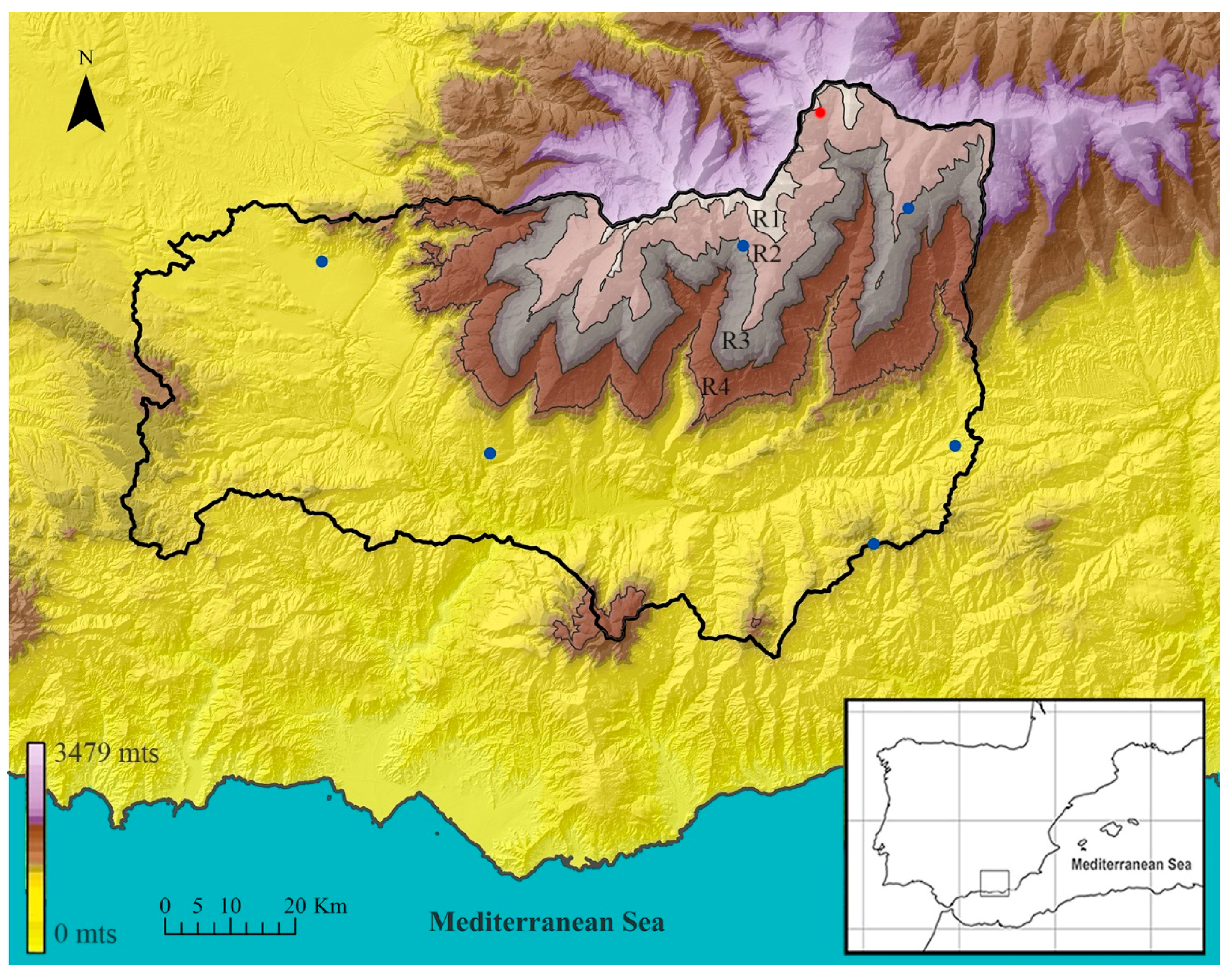
This study was carried out in the Sierra Nevada Mountains, Southern Spain, where one of the greatest wealths of biodiversity in fauna and flora in Europe can be found [21,22]. The highest region of the range was declared a UNESCO Biosphere Reserve in 1986, Natural and National Parks in 1989 and in 1999, respectively). The Guadalfeo river basin upstream the Rules dam was selected for this study (1058 km²) (Figure 1). The area, with an average elevation of 1418.5 m.a.s.l., is characterized by high topographic gradients due to its proximity to the coastline, only 40 km south. Therefore, a combination of alpine and Mediterranean climate conditions can be found. Snowfall appears every year at altitudes over 2000 m.a.s.l. but its presence and distribution is highly variable between consecutive years depending on the meteorological conditions. Precipitation increases with elevation and the mean temperature is usually higher than in alpine climates. The 40-year mean annual values of the precipitation and daily temperature are 630 mm and 12.2 °C, respectively [23]. Global radiation is high throughout the year due to its southern aspect and usual lack of cloud cover, even during winter, despite the cold temperatures and the presence of snow. The rough topography leads to important differences in the instantaneous global radiation between the east and west-facing mountains slopes and, consequently, in the snow albedo values [3].

2.2. Remote Sensing Albedo Data

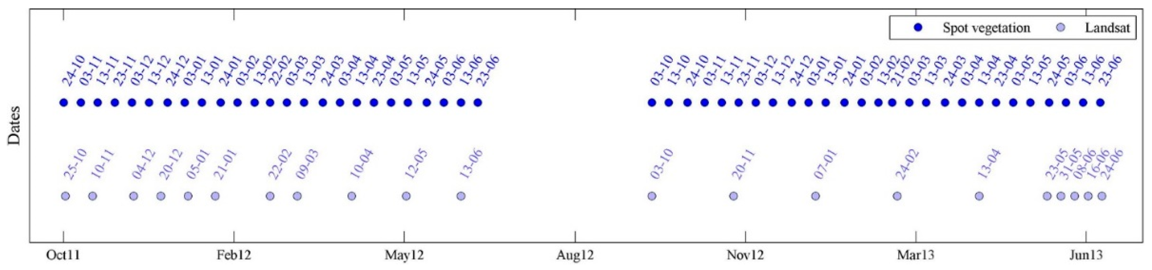
Two sources of remote sensing data were used in this study for the period October 2011–August 2013. The first source consists of the 21 cloud-free multispectral images from Landsat TM5 and ETM+ available from the 2 years analysed; the second source was the SPOT VEGETATION albedo product with 52 available images in the area during the study period (Figure 2).

2.2.1. Landsat Albedo

Twenty one Landsat TM5 and ETM+ scenes were selected within the study period for the cloud free scenes available in order to minimize uncertainties due to heterogeneous atmospheric conditions (Figure 2). Landsat satellites present a temporal resolution of 16 days and 30 × 30 m spatial resolutions. All scenes were subset to form the image of the study area. Both sensors analysed, TM and ETM+, have the same multispectral wavebands with similar spectral coverage. Therefore all the images were processed in the same way.

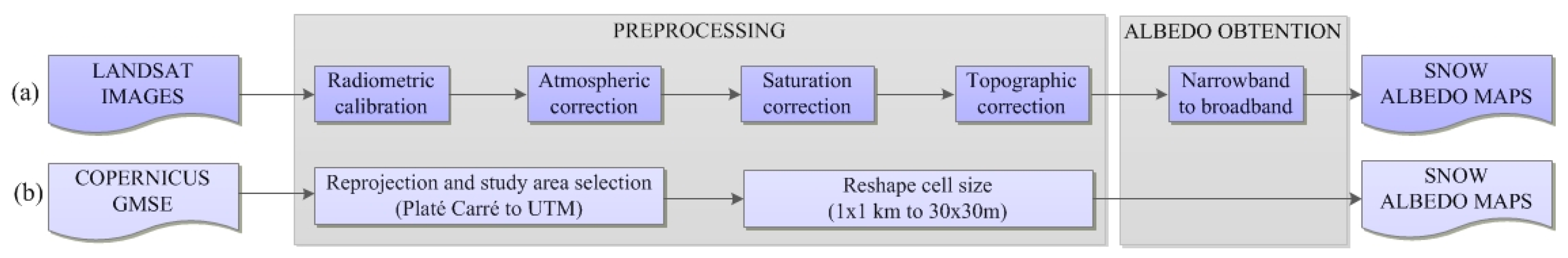
Prior to the snow albedo computation, a pre-processing of the images is required [24]. Figure 3a shows the pre-processing applied in this study that includes the radiometric calibration and the atmospheric, saturation and topographic corrections; in this study, the surface is considered to be Lambertian, that is, the degree of anisotropy of the land surface is not considered and, therefore, the angular correction is not applied [12]. Snow is not a Lambertian surface; nevertheless, some works show this assumption can be adopted without significant errors. Dumond et al. (2010) [25] showed that, for snow surfaces, the anisotropy factor for wavelengths under 1.2 nm is nearly constant and close to the unit; thus, for those wavelengths, the Lambertian assumption does hold. For wavelengths above this 1.2 nm threshold, the anisotropy factor varies depending on the incident/viewing directions; as the TM sensor is for nadir viewing, the direction is always fixed, and the incident direction is approximately the same because of the sensor overpass for the area, and for that, approximately 30°, the anisotropic factor is also close to 1.

Radiometric calibration was achieved through the equations and rescaling factors in Chander et al. (2009) [26].

Atmospheric correction was conducted to retrieve surface reflectance by use of the dark object subtraction (DOS) method, which relates the satellite radiance and the surface reflectance [27,28] by assuming a Lambertian surface and a cloudless atmosphere. Moreover, all the scattering effects are considered to be the same as those of a blackbody within the scene [29]. This dark object is selected from the minimum radiance value of the histogram with at least 200 pixels [30], excluding those pixels in the scene that lie in the shadows produced by the terrain roughness [31]. Thus, fixed values for the downwelling transmittance parameters of the atmosphere for each band are adopted [32] and the upwelling atmospheric transmittance and the diffuse irradiance are both neglected. DOS methods constitute a good alternative when the atmospheric optical properties needed by more complex radiative transference codes (RTCs) are totally or partially unavailable or are of questionable quality [33].

Snow in the Landsat scene where the study site is included constitutes less than 5% in the maximum snow extension and becomes insignificant at the end of the snow season. For this reason, several bands are radiometric saturated, especially in winter when the difference between snow and the rest of land covers in the scene is greater. To correct this saturation, a multivariable correlation analysis between bands is employed to recover the snow-saturated pixels [34].

Regarding the topographic correction, a C correction with land cover separation algorithm was applied [31]. Again, under the Lambertian surface assumption a linear fit between the illumination angle and the different bands reflectance is established. Additionally, the diffuse irradiance is taken into account via a semi-empirical estimation of the C factor. In order to consider the multiple reflective properties of the different vegetative soil covers, the pixels were classified into bare soil and vegetated areas by using the Normalized Difference Vegetation Index (NDVI) [35].

Once the images are corrected, the discrimination of snow-covered areas and the narrowband-to-broadband conversion are applied to generate the snow albedo maps. The separation of snow-covered and snow-free areas was carried out with the normalized difference snow index (NDSI) [15] and the high reflectance of snow in the visible part of the spectrum (Band 1 in Landsat images). In this work, the two thresholds used to discriminate the snow were NDSI > 0.4 and Band 1 > 0.1 [36,37]. The narrowband to broadband conversion was performed following the method of Brest and Goward (1987) [38], based on the numerical integration of the snow spectral albedo curve throughout the shortwave spectrum. In their work, the homogeneous parts in the snow spectral albedo curve were identified and then a given percentage of the total spectrum was assigned to each identified homogeneous interval portion. The different spectral bands of the sensor were used as representative of each one of such parts. This method can be applied to different kinds of mixes surfaces, as the authors showed, including snow areas. Following this, 4 bands (TM2, TM4, TM5, and TM7) of the 6 bands of the TM sensor were used in this study, each one assumed to be representative of the following segments, s1 = 300–725 nm, s2 = 725–1000 nm, s3 = 1000–1400 nm, s4 = 1400–2500 nm (each one of them with approximately constant spectral albedo). The weighting function shown in Equation (1) gives an estimation of the broadband albedo in snow surfaces [38,39].

$$Albedo=0.493\cdot (Band2)+0.203\cdot (Band4)+0.150\cdot (Band5)+0.154\cdot (Band7)$$

(1)

2.2.2. SPOT VEGETATION Albedo

Sixty-eight Geoland-2 SPOT/VGT Albedo products from Copernicus Land Monitoring Service were analyzed along the study period (Figure 2). The temporal and spatial resolutions of the products were 10 days and 1 km × 1 km respectively. From the two albedo variables available in the GMES/Copernicus datasets, the hemispherical albedo (AL-BH) was the one used in this study. It provides the integration of the directional albedo over the illumination hemisphere and assumes a complete diffuse illumination. Moreover, the FLAG sub-product was employed to discriminate snow-covered and some-free pixels. The algorithm used to make this discrimination is also based on the NDSI index, but in this case, adapted to the available band in SPOT VEGETATION [40].

The pre-processing applied to SPOT VEGETATION data is shown in Figure 3b. First, all products were subset to form the image of the study area. Then, as the projection systems used by the model and the SPOT VEGETATION data are different, an automatic routine to re-project the data was implemented in MATLAB. Finally, in order to match the different cell-sizes of both remote sensing data sources, a reshape in the cell size of the available products from 1 km × 1 km to 30 m × 30 m was applied. A nearest neighbor interpolation algorithm was the method employed.

Following this process, the albedo maps are derived for the snow covered pixels determined in the FLAG product.

2.2.3. In Situ Albedo Measurements

In situ snow albedo data are only available from two stations within the study area, but only one of them (Collado Buitreras; see Figure 1) has been operative during the whole study period. It is located at 2867 m.a.s.l. and is being measuring albedo from the winter of 2008 on; the second one has just been operative from the late spring of 2013, out of the study period in this work, and thus was not used.

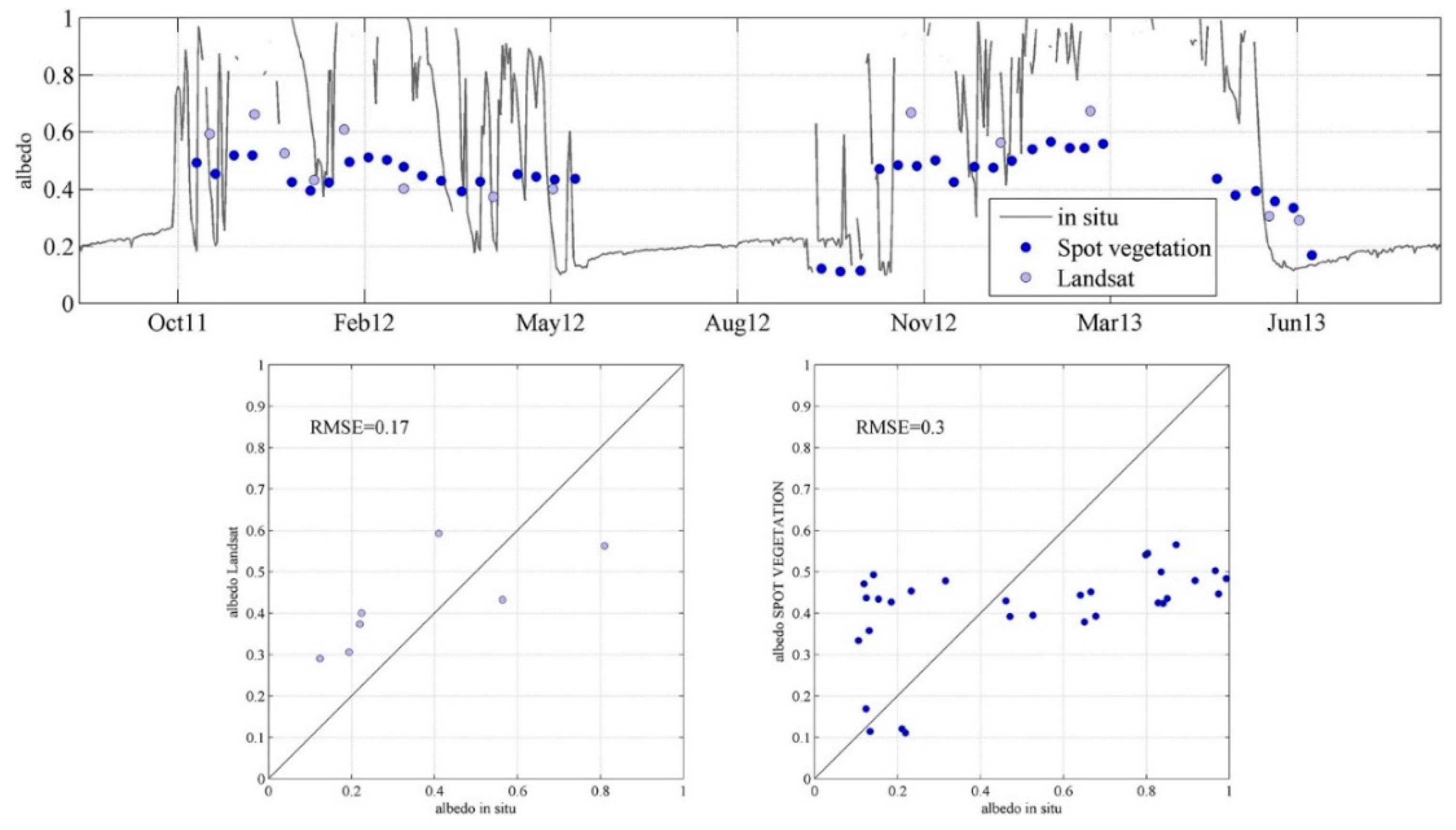
The in situ albedo measurements were used to validate the albedo obtained from the remote sensing sources. Only 7 of the 21 Landsat scenes and 35 of the 52 SPOT VEGETATION scenes could be used in the validation process, since the in situ albedo measurement was out of range in the rest of them. For comparison, the instantaneous in-situ albedo value measured at 10:40 a.m. (GMT+1), approximately the acquisition time of Landsat scenes, was selected; in the case of the SPOT VEGETATION validation, an averaging of the instant measurements corresponding to the 10-days windows of the sensor’s scene was obtained.

2.3. Meteorological Data

Daily meteorological observed data of precipitation, temperature, wind velocity, radiation and relative humidity recorded at six weather stations covering the altitudinal gradient in the area (Figure 1) were used in this study. These meteorological data were used as inputs to the hydrological model WiMMed (Wathershed Integrated Model in Mediterranean Environments), whose snow module is operational over this area from previous works [9,14,37,41]. Specific interpolation algorithms were used to distribute the point measurements of the meteorological variables over the whole study area. Precipitation, temperature, humidity and wind speed are interpolated by means of a squared inverse of distance weight method (IDW2); a correction based on the observed altitudinal gradients is included for temperature and precipitation. These algorithms were tested and validated in the study area [42] and are currently used in the operational version of the snow and hydrological model in the associated watersheds. Moreover, for radiation, a physical model based on the clearness index and the diffuse/direct fraction with inclusion of the different topographic effects is applied [3]. Finally, for the atmospheric emissivity, a specific formulation for mountainous areas that was locally validated at the study site is used [43].

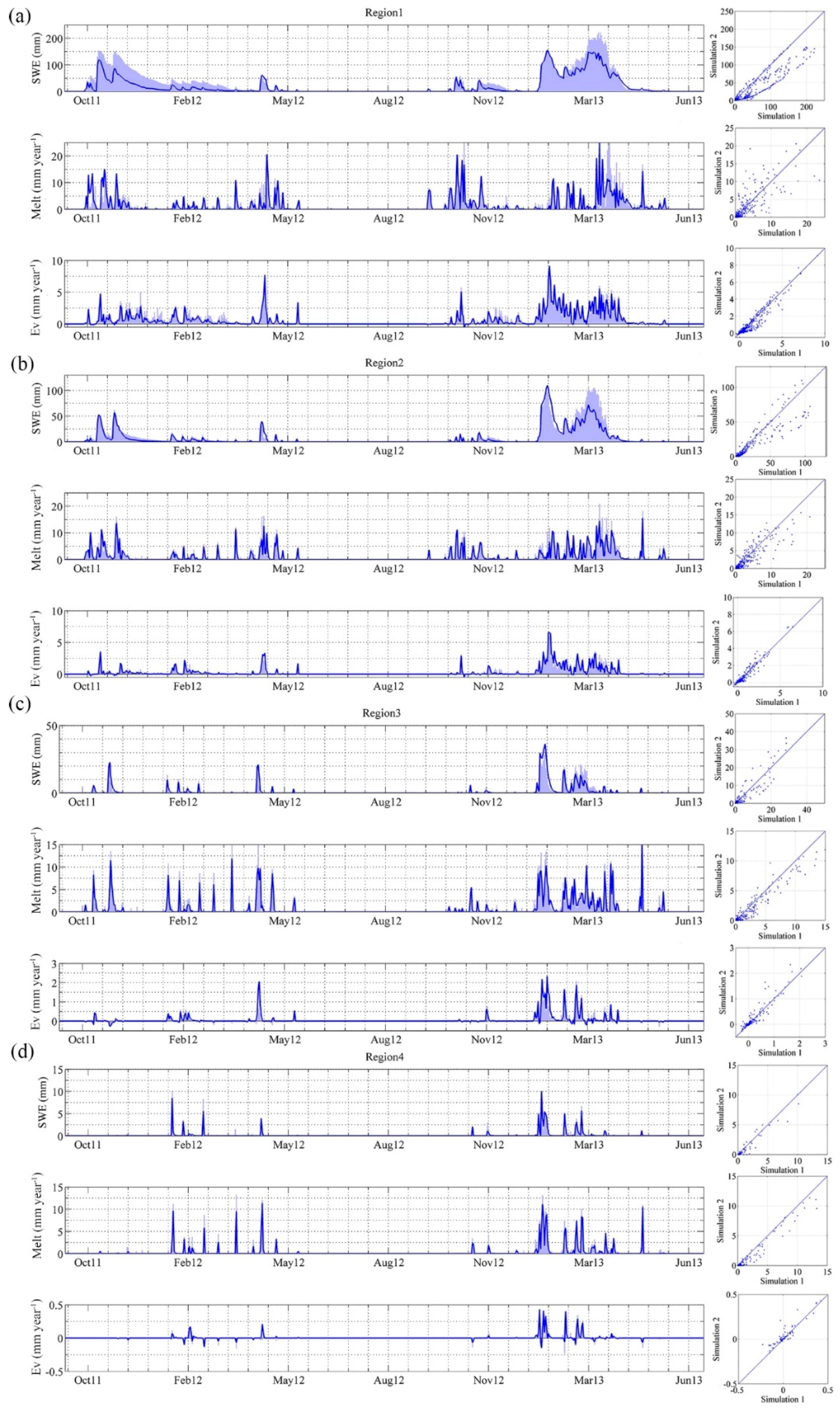
The study period covers two hydrological years, from September 2011 to August 2013. To analyse the most vulnerable changes in snow albedo, only the area usually covered by snow within the watershed, located above 1500 m.a.s.l., was selected for the study. Moreover, this study area has been divided into four regions related to the altitude range: 3500–3000 m.a.s.l. (R1), 3000–2500 m.a.s.l. (R2), 2500–2000 m.a.s.l. (R3) and 2000–1500 m.a.s.l. (R4) (Figure 1).

Table 1. Main topographic and annual climatic features of the study area and each altitudinal regions calculated on a 10 m × 10 m DEM supplied by the Regional Andalusian Government.

	Area (km2)	Altitude (m.a.s.l.)	Slope (mm−1)	Precipitation (mm)	Snowfall (mm)	Tmean (°C)	Tmax (°C)	Tmin (°C)
REGION 1	15.8 (5%)	3110.8	0.22	935	759	2.9	16.685	−13.95
REGION 2	100.6 (33%)	2727.5	0.19	834	565	4.8	18.3	−11.5
REGION 3	124.8 (41%)	2249.4	0.21	735	323	7.4	20.8	−8.15
REGION 4	151.8 (51%)	1744.6	0.22	637	129	10.3	24.0	−4.5
TOTAL	393.0	2211.4	0.21	731	328	7.7	21.1	−7.8

shows the main topographic and mean annual climatic features describing the study area and each altitudinal region, Region 3 being representative of the average features of the study area.

2.4. Snow Modelling

The snowmelt-accumulation model developed by Herrero et al. (2009) [5] is a physical model based on a point mass and energy balance, spatially distributed by means of depletion curves [37,41]. This model was created and mainly tested in Mediterranean and semiarid high mountains.

The point model assumes a one-layered uniform snowpack. In the control volume defined by the snow column per unit area, which has the atmosphere as an upper boundary and the ground as a lower one, the water mass and energy balance can be expressed by Equations (2) and (3):

$$\frac{dSWE}{dt}=R-E+W-M$$

(2)

$$\frac{d(SWE\cdot u)}{dt}=\frac{dU}{dt}=K+L+H+G+R\cdot u_R-E\cdot u_E+W\cdot u_W-M\cdot u_M$$

(3)

where SWE (snow water equivalent) is the water mass in the snow column, and u is the internal energy per unit of mass (U for total internal energy). In the mass balance, R defines the precipitation rate; E is water vapour diffusion rate (evaporation/condensation); W represents the mass transport rate due to wind; and M is the melting water rate. On the other hand, regarding energy fluxes, K is the solar or short wave radiation; L the thermal or long-wave radiation; H the exchange of sensible heat with the atmosphere rate; G the heat exchange with the soil rate; and u_R, u_E, u_W and u_M are the advective heat rate terms associated with each one of the mass fluxes involved in Equation (2).

In the mass balance Equation (2), W is disregarded due to the quick snow metamorphosis observed at the study area, that compacts the snowpack and reduces its mobility. G is not considered either in the energy balance equation, being usually considered a secondary term per se in this balance [44] Shortwave radiation (K) is calculated through the measured downwelling shortwave radiation flux and the albedo. Longwave radiation is calculated by means of an empirical formulation for the atmospheric longwave emissivity, locally validated in the area [43]. Finally, H is modelled as a diffusion process [45].

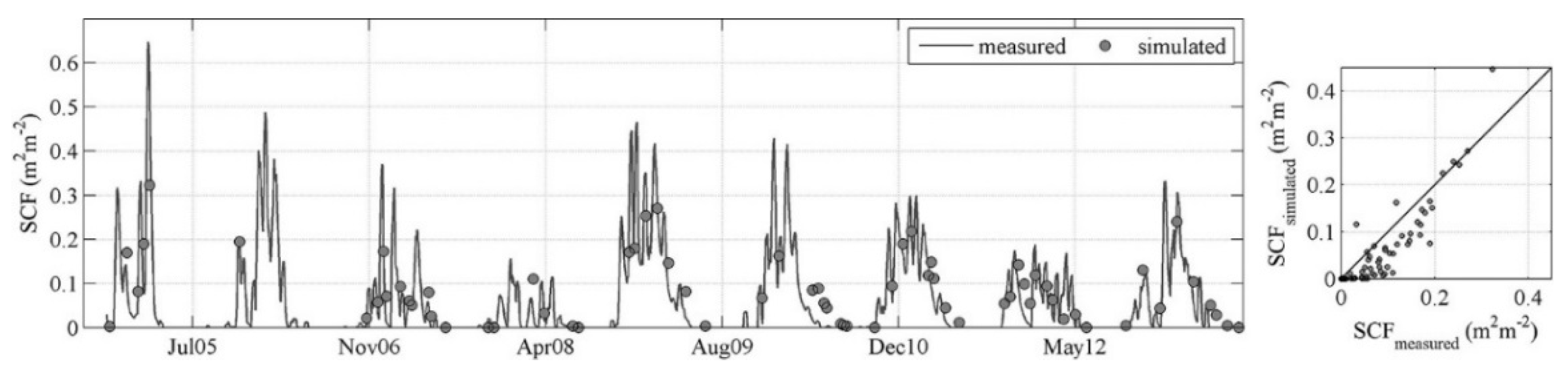
The point model is then distributed over the study area using a 30 m × 30 m rectangular grid where the snow energy balance is performed over each cell. The parameterization of subgrid processes is carried out by defining depletion curves, which are empirical functions that relate the fraction of cell area covered by snow with some other snow state variable. They allow quantification of the decrease in snow cover area within the cell to take into account the reduction of the surface area implied in the energy-mass balance. Because of the annual occurrence of different snowmelt cycles during the snow season and their variability between years, different depletions curves were proposed for each kind of melting/accumulation cycle identified in the area. The model has been previously calibrated and validated over the area in term of snow cover fraction (SCF) obtained from Landsat TM and ETM+ using a spectral mixture (Figure 4) [41].

2.5. Comparison between Landsat and SPOT VEGETATION Albedo Values

Snow albedo values retrieved from both data sources were used to obtain distributed daily series of snow albedo of 30 m × 30 m-cell size from October 2011 to August 2013. For this, time intervals between two consecutive images were filled by assuming the acquisition date value during N days before and afterwards; then, linear interpolation was applied for the rest of the intermediate period. N was fixed as 10 and 5 days for Landsat and SPOT VEGETATION, respectively.

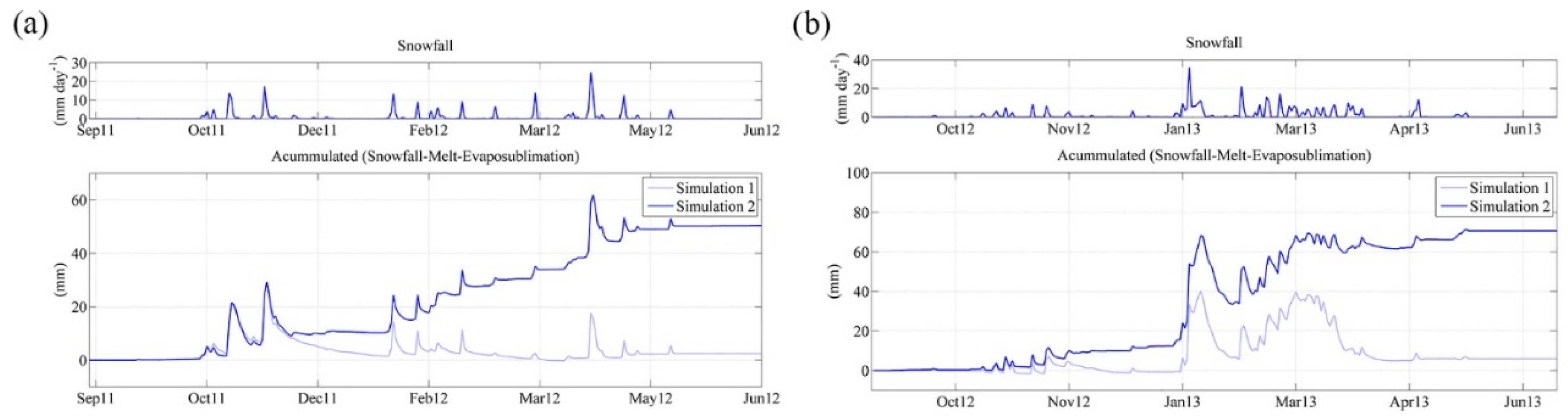
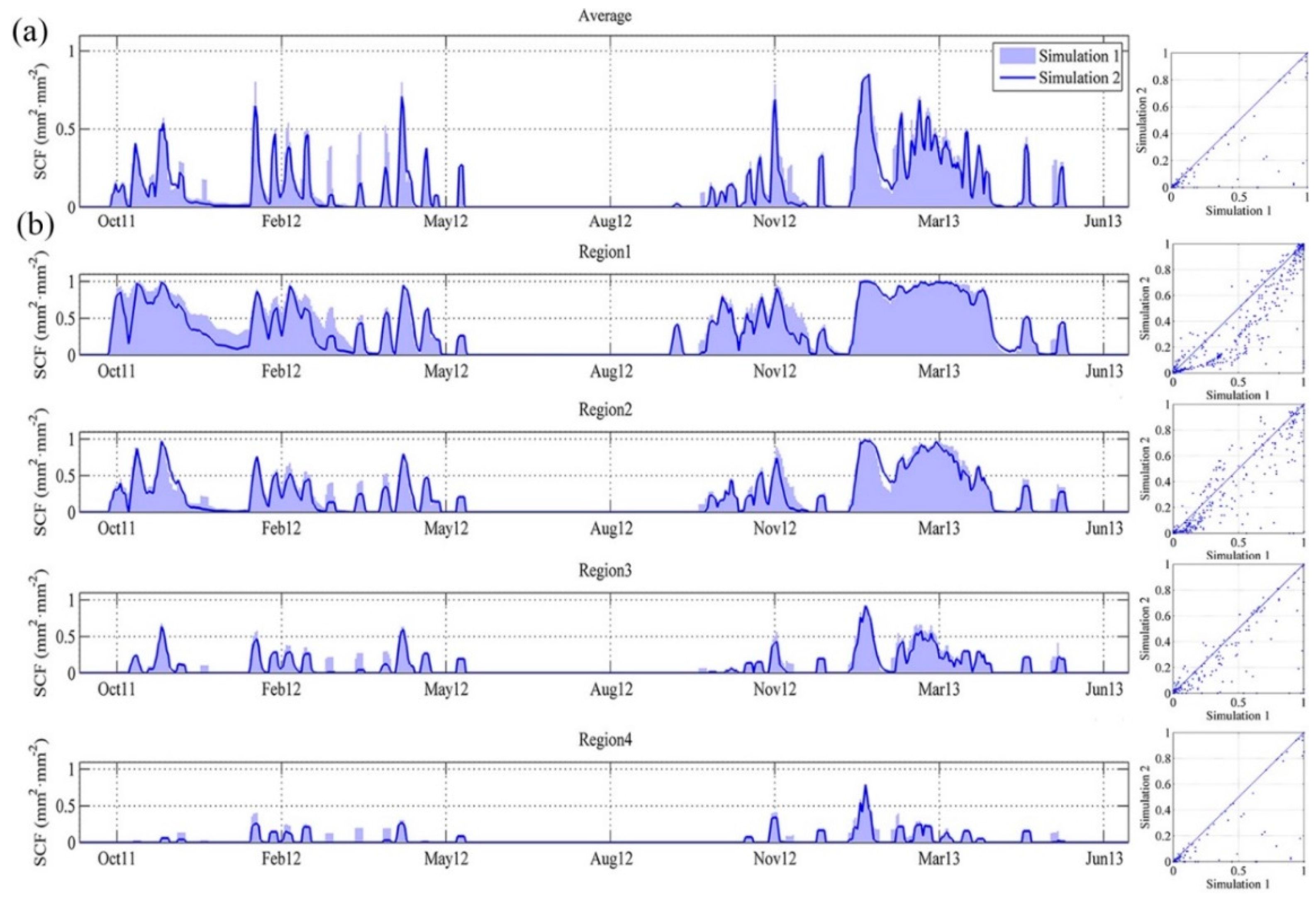
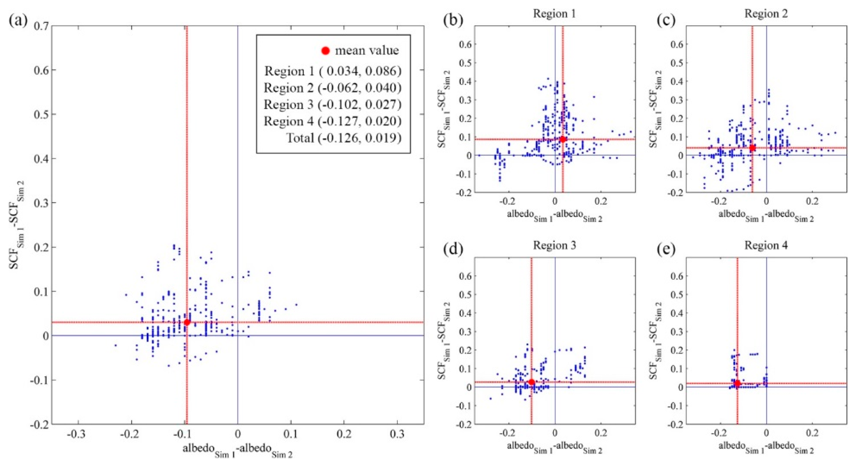
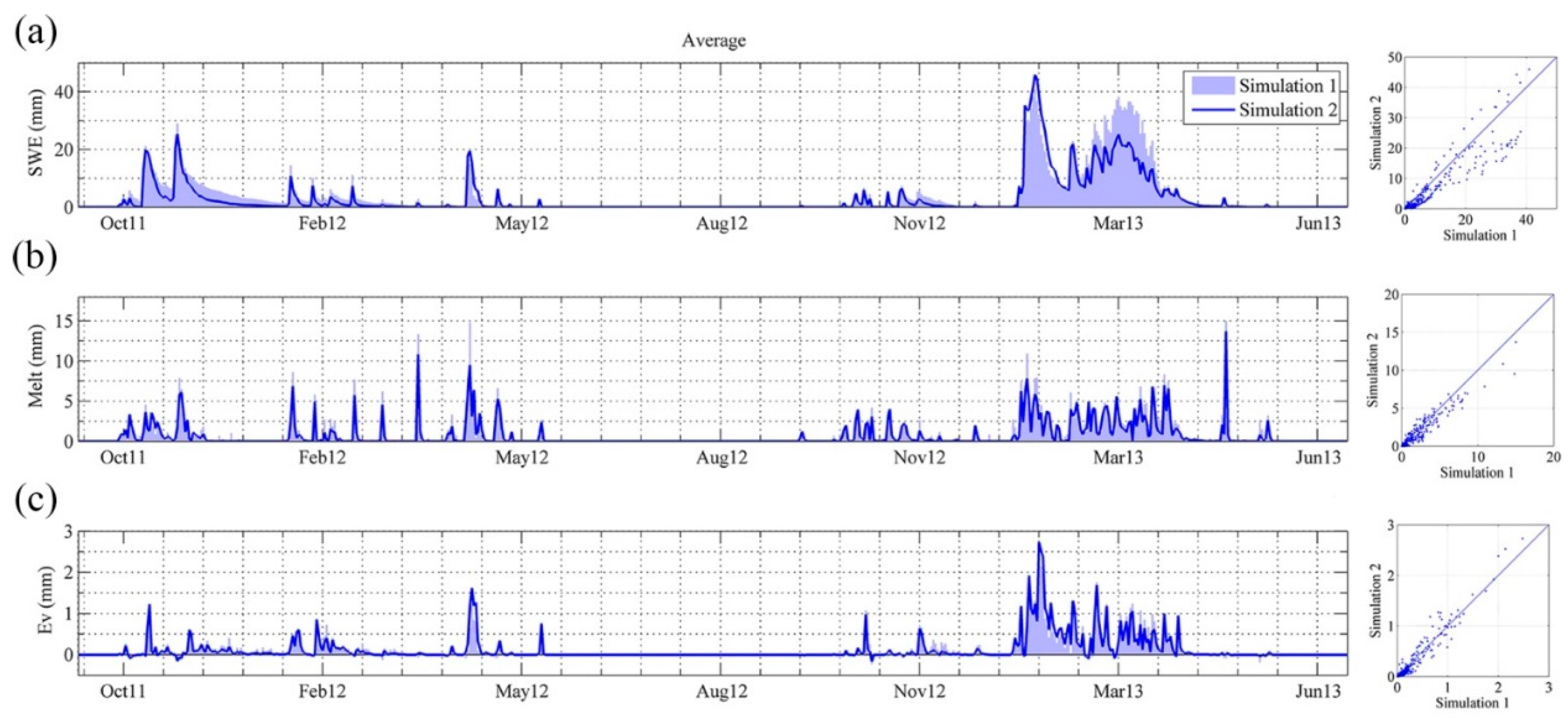
The resulting albedo maps were used as input values in the snow module of WiMMed model, operational at the study site, to assess albedo resolution influence on the snow regime. Two simulations were performed: Simulation 1 and 2, using albedo values obtained from Landsat TM, ETM+, and SPOT VEGETATION dataset, respectively. The model results analyzed in each simulation were the daily values of the following snow variables: mean snow cover fraction (SCF), mean snow water equivalent (SWE), snowmelt (Melt) and evapo-sublimation (Ev).Their average values over the whole study area are presented in this work, together with their average values over each one of the four altitudinal regions previously defined.

The SCF results shown for each simulation and area correspond to the model estimations; the indirect information about SCF values that both remote sensing sources provided has not been used in this work, since the main goal was assessing the albedo source influence. However, some disagreement may appear between the model detection of snow (SCF different from zero) and the image detection (albedo different from zero); in such cases, the SCF estimated value was maintained. To avoid the associated non-continuity in the calculations, the following criteria were followed: when SCF results different from zero - whereas when the snow albedo is equal to zero, a minimum albedo value of 0.4 is assigned by the model, provided SCF is higher than 0.5; similarly, when the calculated SCF is equal to zero but the snow albedo is different from zero, the snow albedo data is ignored and a zero value is adopted.

Finally, to assess the influence of the fraction of mixed pixels (SCF < 1) on the results during the melting periods, the SCF values retrieved by Pimentel et al. (2014) [41] from Landsat images by means of spectral mixture analysis were used for the Landsat acquisition dates (Figure 2).

3. Results

3.1. Snow Albedo Time Series during the Study Period

Figure 5 shows both Landsat (L) and SPOT VEGETATION (SV) snow albedo daily series used as input in Simulation 1 and Simulation 2, respectively, averaged over the whole study site (Figure 5a) and each one of the four altitudinal regions identified in this work (Figure 5b), during the study period (October 2011-August 2013); the periods with zero albedo correspond with no-snow conditions in the study area (2012/05/28–2012/09/16; 2013/03/28–2013/05/31; 2013/06/07–2013/06/16; 2013/06/23–2013/08/31). Both series experiment a similar evolution when averaged over the whole study area (Figure 5a), with coincident increasing and decreasing phases during the snow seasons. L-albedo is generally lower than SV-albedo when averaged over the study area, with a mean value for the study period of 0.11 against 0.21; the difference is higher during warm periods and increases from the beginning of spring to summer. L-albedo exhibits a maximum average value of 0.36 and a minimum of 0.01 in March 2013, respectively; for SV-albedo, these values are 0.34 and 0.13, in the same periods.

The regional analysis (Figure 5b) shows a clear decrease of the average snow albedo with the elevation, with mean average L-albedo values of 0.38, 0.27, 0.08, 0.01 for Region 1, 2, 3 and 4, respectively, and 0.38, 0.35, 0.18, 0.14 mean SV-albedo values for each region too. Although mean L-albedo values are always lower than those from SV-albedo, the difference increases as altitude decreases, as can be easily observed from the Figure 5. Again, the difference is higher during spring and summer, where the presence of mixed pixels is more significant.

The validation of the albedo values obtained from remote sensing sources is shown in Figure 6 for each one of the available dates. As can be seen, the obtained values fall within the observed range, taking into account the fact that the sensor-albedo values correspond to 1 × 1 km and 30 × 30 m pixel areas from SPOT VEGETATION and Landsat respectively, whereas the in situ albedo values are point measurements. The mixed nature of the areas represented by each pixel in the study site during long periods justifies these lower values, since it is a surface value against a snow point value, and the pixel is not just a snow surface, but a heterogeneous one. Only pure snow pixels could be approximate in this comparison. A RMSE of 0.17 and 0.30 was found between in situ values and each source respectively.

3.2. Simulated Snow Cover Fraction

The evolution of the daily mean snow cover fraction simulated from both L and SV-albedo values (Simulation 1 and 2, respectively) throughout the study period is shown in Figure 7. As in Section 3.1, the results are represented as the average values over the whole study area (Figure 7a) and over each region (Figure 7b). Very close values for both simulations are found in all the cases, with generally similar or lower SV-SCF (Simulation 2), with a mean difference from L-SCF of 0.02 m²∙m⁻² (Figure 7a), and maximum differences between 0.38 and 0.33 associated to the occurrence of isolated snowfall events in spring (March–April 2012 and May 2013) and during some of the intermediate fall-winter melting cycles (December 2011, November 2012) (Figure 7).

Figure 8 shows the difference between the simulated daily L and SV-SCF values against the difference between the daily L and SV-albedo values, both variables averaged over the whole study area (Figure 8a). From Figure 8b–e, it can be observed that the mean difference of L and SV-albedo values shifts from a positive value in Region 1 (0.034) to negative values in the rest of regions (−0.062, −0.102, −0.127 respectively), with an increasing trend in their absolute value as the altitude decreases (red axes in the graphs), whereas the mean differences found between L-SCF and SV-SCF values are always positive, also clearly dependent on the altitude region, with higher values in Regions 1 and 2, where snowfall has a stronger presence and persistence, and a general decreasing trend as altitude is lower. The mean SCF difference found ranges from 0.086 in Region 1 to 0.020 in Region 4. This is related to the importance of mixed pixels in each region; the spectral mixture analyses performed on the Landsat scenes during the study period following Pimentel et al. (2015) [41] resulted in the number of mixed pixels being equivalent to 34%, 55%, 89% and 34% of the area in Region 1, Region 2, Region 3 and Region 4, respectively.

The results also show the non-linearity of the snow albedo influence on the simulated SCF values, with most of the points belonging to the upper left quadrant from the 0-0 axes (blue axes in graphs in Figure 8), but also presence of points in both the upper right and lower left quadrants. The upper left domain in these graphs correspond to conditions with high significance of the shortwave components of the energy balance for the snow evolution (a lower snow albedo involves higher snow cover fraction), whereas the upper right and lower left domains correspond to situations in which other energy terms have more influence on the mass balance (for example, the longwave component) or isolated snowfall events take place.

3.3. Simulated Daily Snow Water Equivalent and Snowmelt/Evapo-Sublimation Fluxes

The evolution of the daily mean snow water equivalent (SWE), snowmelt (Melt) and evapo-sublimation (Ev) fluxes simulated from both L and SV-albedo values (Simulation 1 and 2, respectively) throughout the study period is shown in Figure 9 and Figure 10. As in previous sections, the results are represented as the average values over the whole study area (Figure 9) and over each region (Figure 10).

In all the cases, the trend of evolution is quite similar; however, some differences are found during certain periods, which are higher for Regions 1 and 2, as expected.

In general, the use of SV-albedo values results in lower values of both daily average SWE and snowmelt over the whole study site (Figure 9a,b), whereas the evapo-sublimation is less clearly biased, as the dispersion graphs in Figure 9c show. The same can be observed in the altitudinal regions results (Figure 10), except in Region 1, whose dispersion graphs show the reverse results, with some dispersion over the 1:1 line for snowmelt but lower values of SV-evapo-sublimation than those obtained for L-evapo-sublimation. In this region, the shift of SV-SWE is clear, with significantly lower values than those of L-SWE.

Finally,

Table 2. Average values of the main component in the water budget over the whole study area and over each of the regions throughout the two study years, 2011–2012 and 2012–2013, and the complete period.

		Year 2011–2012		Year 2012–2013		Accumulated values 2011–2013
		Simulation 1	Simulation 2	Simulation 1	Simulation 2	Simulation 1	Simulation 2
REGION 1	Pre (mm)	585		1248		1833
	Sn (mm)	560		950		1510
	Melt (mm)	384.6	369.8	668	598	1052.6	968
	Ev (mm)	184.3	132.8	266	247.4	450.3	380.2
REGION 2	Pre (mm)	516		1117		1633
	Sn (mm)	426		705		1131
	Melt (mm)	358.7	294.8	542.3	451.3	901	746.1
	Ev (mm)	57.2	52.3	137.1	132.2	194.3	184.5
REGION 3	Pre (mm)	450		989		1439
	Sn (mm)	239		408		647
	Melt (mm)	226.6	172.7	363.7	292.3	590.3	465
	Ev (mm)	6.6	10.1	28.3	29.3	34.9	39.4
REGION 4	Pre (mm)	385		860		1245
	Sn (mm)	93		162		255
	Melt (mm)	98.5	66.2	181.3	143.6	279.8	209.8
	Ev (mm)	-0.3	0.4	1.8	2.6	1.5	3
TOTAL	Pre (mm)	447		982		1429
	Sn (mm)	243		413		656
	Melt (mm)	217.1	170.6	351.2	287.9	568.3	458.5
	Ev (mm)	24	22.1	55.4	54.1	79.4	76.2

shows the accumulated values of snowmelt and evapo-sublimation during both years under study, together with the annual precipitation and snowfall, averaged over the whole study site and each one of the altitudinal regions in this work. As can be observed, the simulation with the L-albedo values results in a higher annual snowmelt than that obtained from the SV-albedo values for both years and all the regions, whereas the annual evapo-sublimation values are similar in all the cases. However, the simulation with the SV-albedo produces a closure error of the annual water balance from the snowfall (snowfall minus the sum of the associated snowmelt and evapo-sublimation) up to 10% in some cases, as opposed to the 1% obtained by the simulation with the L-albedo. This is a numerical effect of the lower values of SV-SCF (see Section 3.2), associated with the internal threshold of the snow model to accumulate or neglect snowfall occurring in a cell with initial SCF equal to zero. In a given pixel, SWE values lower than 0.1 mm at the end of a time step in the calculation procedure are assumed to melt and infiltrate through the soil. These conditions are usually found at the end of melting phase, but also when there is snowfall over bare soil. Consequently, a low-intensity and isolated snowfall event will not be taken into account in the energy balance over the snowpack in a larger number of cells when SCF is underestimated; however, this water amount will be considered by the model in the global water budget as it is included in the infiltration rate in such cells (Figure 11).

4. Discussion

The results shown in the previous section demonstrate the influence of the spatial resolution of the snow albedo measurements by remote sensing on the modeling of snow dynamics in semiarid regions.

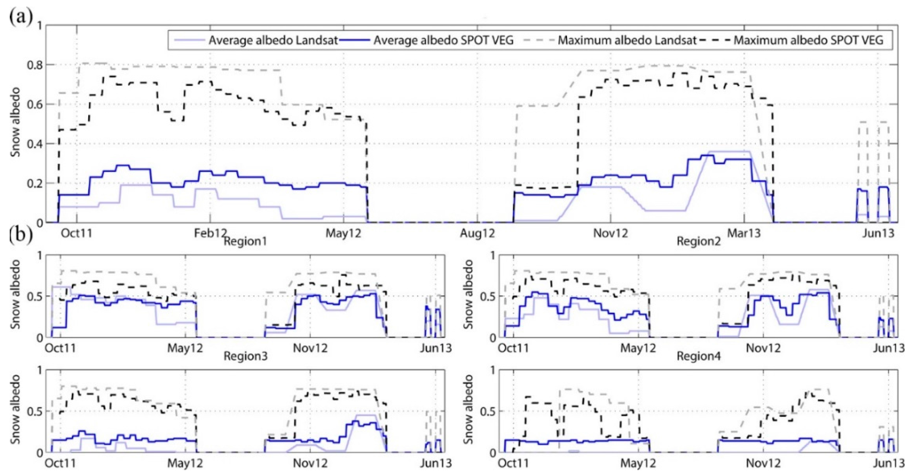
The average over the whole region of the distributed snow albedo obtained from both data sources show lower values than those available in the literature, usually between 0.4 for dirty snow to 0.9 to clean snow [45]; this is due to the scale effect when comparing point field measurements with an average value corresponding to the whole pixel size of the corresponding sensor. Generally higher snow albedo values are found for the average SV-albedo, but as seen in Figure 5, higher maximum daily values are found for L-albedo (dotted light line) when compared to the maximum found for SV-albedo. This is a direct spatial effect due to the higher presence of pure snow pixels (with higher albedo) in the Landsat than in the SPOT VEGETATION images in these semiarid environments. The comparison among Regions confirms this effect, with daily averaged values being more similar between both data sources in Region 1, where snow is predominant, and more differences in the rest of the regions; the reverse can be observed when comparing the daily maximum pixel value for each sources, due to the cell size factor already described.

Nevertheless, the differences found between both snow albedo sources can be biased, for different reasons. First, the retrieval of daily series of snow albedo maps includes a different way to discriminate between snow and no-snow pixels depending on the source, and this initial difference induces disagreement in the area for which albedo is retrieved.

Secondly, and more importantly, at the study site the presence of mixed pixels is much higher in the SPOT VEGETATION than the Landsat images. A mixed pixel is not completely covered by snow, and thus, its retrieved snow albedo is the result of the signal from the true snow-covered area in the pixel and the rest of the covers present in its area. This fact generally reduces the retrieved snow albedo in the mixed pixels, whose presence is really significant over semiarid mountainous areas during those periods in which snow is distributed in patches. When the mixed pixels identified in the Landsat images are eliminated, the mean increase of the averaged albedo value is 35%, which serves as an example of how the presence of these mixed pixels greatly affects the finally retrieved albedo values. This restriction is more critical in SPOT VEGETATION albedo products, since their spatial resolution (1 km × 1 km) increases the presence of these mixed pixels. This induces two opposite biases: pixels including snow in medium-low proportion will get an albedo value higher than that referring to the no-snow area that would found at a 30 m × 30 m scale; pixels including snow in a high-medium proportion will have a lower albedo value than that referring to the pure snow area that would be found at a 30 m × 30 m scale. Finally, it must be taken into account that the SPOT VEGETATION products only cover the visible and near infrared ranges of the spectrum and not the whole shortwave infrared radiation range.

The results show the significant effect of the albedo source on the estimated SCF during the study period, effects reported by other authors [46], and the associated SWE and snowmelt and evapo-sublimation fluxes, and how these effects change depending on the altitudinal region in the study. On a daily basis, SV-albedo results underestimate the SWE when compared to the L-SWE values, and this produces lower values for the associated snowmelt in most of the days; the impact on the evapo-sublimation does not follow a fixed trend and is only relevant in Region 1, in which snow is clearly dominant. Previous works also showed a significant impact on the snowmelt rates with even small changes in the snow albedo value [47,48]. This shift in the calculations results in a higher error for the water closure of the snowfall balance due to numerical effects of the internal decision-making tree in the snow model; however, taking into account that this “lost” snowfall is converted into rainfall, the underestimation of snowmelt very likely produces an overestimation of the infiltration in the area, which minimizes the impact on the water balance of the total annual precipitation (rainfall + snowfall). This has direct implications for the use of one source of albedo data or another, depending on which final objective the simulation has: the direct observation and monitoring of the snowpack evolution, the influence of the snow regime on the annual water balance (for water resource planning) or operational flood-alert systems in the associated basins. In the first case, L-albedo is recommended for snow modeling; in the second, both albedo sources very likely provide similar results, and then the advantages of a direct albedo product availability as the SV-albedo must be considered in the final decision. The third case recommendation is dependent on the impact of snowmelt on the runoff generation and travel time and peak flow of significant floods in the area.

5. Conclusions

The influence of the spatial resolution of the albedo input on snow modeling has been studied in a Mediterranean mountainous area representative of snow domains in semiarid regions. For this purpose, the two remote sensing sources analyzed, Landsat and SPOT VEGETATION, with significantly different sensor pixel sizes, were used to retrieve daily maps of snow albedo, which served as inputs for the operational snow model available at the study site, the Sierra Nevada Range in southern Spain.

The results have shown a mean increase in the averaged retrieved snow albedo series from SPOT VEGETATION product of 0.1 when compared to the Landsat source, which is distributed along the altitudinal range, with higher values in the regions dominated by the snow presence. The scale effects associated with the pixel size of the albedo source are first identified in the simulated 2-year period as a shift of the estimated SV-SCF values from the estimated L-SCF. These lower SV-SCF values represent an underestimation of the presence of snow and thus all the snow variables are affected in the simulation process. This shift ranges from 0.086 m²/m² in the highest altitudinal region (over 3000 m.a.s.l.) to 0.020 m²/m² in the lowest altitudinal region (2000–1500 m.a.s.l.).

The impact on the water balance at the study area is represented by the simulated daily SWE values using both snow albedo series, as well as the associated daily water fluxes from the snowpack, snowmelt and evapo-sublimation. SV-SWE values were generally lower than L-SWE values, as the associated daily snowmelt values, whereas the effects of the daily evapo-sublimation did not follow a given trend. However, since the latter represent a lower fraction of the snowfall water balance, the snowmelt underestimation by the SV-albedo simulation resulted in a 10% error of the water balance closure of the snowfall on an annual basis. As expected from the SCF values, these results are dependent on the altitudinal region considered.

On a daily basis, L-albedo is recommended in these highly heterogeneous areas when a direct monitoring of the snowpack evolution is intended; however, the availability of direct albedo products provided by larger-scale sensors, such as the SPOT VEGETATION product analyzed in this work, is worth being considered when water resource planning for the medium or long term is the final goal of the calculation process, since the closure error found may be similar to that for Landsat when the water balance is performed on the total precipitation. Moreover, in all cases, further improvement of the results obtained from both sources is expected from additional techniques, such as assimilation, effective calibration of the model associated with each data source, or further downscaling of the albedo product. For applications devoted to short-term forecasting of hydrological variables in snow basins, further analysis must be done.

The use of products such as SPOT VEGETATION is promising, although their direct application in medium-size or highly heterogeneous areas must be specifically assessed, as these results have shown. However, their easy manipulation is a positive point in the decision-making process for operational purposes.

References

1. Blöschl, G. The influence of uncertainty in air temperature and albedo on snowmelt. Nord. Hydrol. 1991, 22, 95–108. [Google Scholar]
2. Dozier, J.; Painter, T.H. Multispectral and hyperspectral remote sensing of alpine snow properties. Annu. Rev. Earth Planet. Sci. 2004, 32, 465–494. [Google Scholar] [CrossRef]
3. Aguilar, C.; Herrero, J.; Polo, M.J. Topographic effects on solar radiation distribution in mountainous watersheds and their influence on reference evapotranspiration estimates at watershed scale. Hydrol. Earth Syst. Sci. 2010, 14, 2479–2494. [Google Scholar] [CrossRef]
4. Barnett, T.P.; Adam, J.C.; Lettenmaier, D.P. Potential impacts of a warming climate on water availability in snow-dominated regions. Nature 2005, 438, 303–309. [Google Scholar] [CrossRef] [PubMed]
5. Herrero, J.; Polo, M.J.; Moñino, A.; Losada, M.A. An energy balance snowmelt model in a Mediterranean site. J. Hydrol. 2009, 371, 98–107. [Google Scholar] [CrossRef]
6. Jordan, R. A One-dimensional Temperature Model for a Snow Cover: Technical Documentation for SNTERERM.89; Special Report 91–16; US Army Corps of Engineers, Cold Region Research & Engineers Laboratory: Hanover, NH, USA, 1991. [Google Scholar]
7. Marks, D.; Dozier, J. Climate and energy exchange at the snow surface in the alpine region of Sierra Nevada. 2 Snow cover energy balance. Water Resour. Res. 1992, 28, 3043–3054. [Google Scholar] [CrossRef]
8. Egüen, M.; Aguilar, C.; Herrero, J.; Millares, A.; Polo, M.J. On the influence of cell size in physically-based distributed hydrological modelling to assess extreme values in water resource planning. Nat. Hazard. Earth Syst. Sci. 2012, 12, 1573–1582. [Google Scholar] [CrossRef]
9. Dozier, J.; Schneider, S.R.; McGinnis, D.F. Effect of grain size and snowpack water equivalence on visible and near.infrared satellite observations of snow. Water Resour. Res. 1981, 17, 1213–1221. [Google Scholar] [CrossRef]
10. Hall, D.K.; Riggs, G.A.; Salomonson, V.V. Development of methods for mapping global snow cover using moderate resolution imaging spectroradiometer data. Remote Sens. Environ. 1995, 54, 127–140. [Google Scholar] [CrossRef]
11. Kimes, D.S.; Holben, B.N. Extracting spectral albedo from NOAA-0 AVHRR multiple view data using an atmospheric correction procedure and an expert system. Int. J. Remote Sens. 1992, 13, 275–289. [Google Scholar] [CrossRef]
12. Liang, S. Narrowband to broadband conversions of land surface albedo I Algorithms. Remote Sens. Environ. 2000, 76, 213–238. [Google Scholar] [CrossRef]
13. Riaño, D.; Chuvieco, E.; Salas, J.; Aguado, I. Assessment of Different Topographic Corrections in Landsat-TM Data for Mapping Vegetation Types. IEEE T. Geosci. Remote. 2003, 41, 1056–1061. [Google Scholar] [CrossRef]
14. Pimentel, R.; Herrero, J.; Zeng, Y.; Su, Z.; Polo, M.J. Study snow dynamics at subgrid scale in semiarid environment combining terrestrial photography data assimilation techniques. J. Hydrometeorol. 2015, 16, 563–578. [Google Scholar] [CrossRef]
15. Pimentel, R.; Herrero, J.; Polo, M.J. Terrestrial photography as an alternative to satellite images to study snow cover evolution at hillslope scale. Proc. SPIE. 2012. [Google Scholar] [CrossRef]
16. McCabe, M.F.; Eric, F.W. Scale influences on the remote estimation of evapotranspiration using multiple satellite sensors. Remote Sens. Environ. 2006, 105, 271–285. [Google Scholar] [CrossRef]
17. Gómez-Giráldez, P.; Aguilar, C.; Polo, M.J. Natural vegetation covers as indicators of the soil water content in a semiarid mountainous watershed. Ecol. Indic. 2014, 46, 524–535. [Google Scholar] [CrossRef]
18. Norman, J.M.; Anderson, M.C.; Kustas, W.P.; French, A.N.; Mecikalski, J.R.; Torn, R.D.; Diak, G.R.; Schmugge, T.J.; Tanner, B.C.W. Remote sensing of surface energy fluxes at 101 -m pixel resolutions. Water Resour. Res. 2003. [Google Scholar] [CrossRef]
19. Anderson, M.C.; Norman, J.M.; Diak, G.R.; Kustas, W.P.; Mecikalski, J.R. A two-source time integrated model for estimating surface fluxes using thermal infrared remote sensing. Remote Sens. Environ. 1997, 60, 195–216. [Google Scholar] [CrossRef]
20. Roy, D.; Ju, J.; Lewis, P.; Schaaf, C.; Gao, F.; Hansen, M.; Lindquist, E. Multi-temporal MODIS–Landsat data fusion for relative radiometric normalization, gap filling, and prediction of Landsat data. Remote Sens. Environ. 2008, 112, 3112–3130. [Google Scholar] [CrossRef]
21. Heywood, V.H. The Mediterranean flora in the context of world biodiversity. J. Hydrol. 1995, 371, 98–107. [Google Scholar]
22. Anderson, R.S.; Jiménez-Moreno, G.; Carrión, J.S.; Pérez-Martínez, C. Postgracial history of alpine vegetation, fire and climate form Lguna de RíoSeco, Sierra Nevada, southern Spain. Quat. Sci. Rev. 2011, 30, 1615–1629. [Google Scholar] [CrossRef]
23. Pérez-Palazón, M.J.; Pimentel, R.; Herrero, J.; Aguilar, C.; Perales, J.M.; Polo, M.J. Extreme values of snow-related variables in Mediterranean regions: Trends and long-term forecasting in Sierra Nevada (Spain). Proc. IAHS 2015, 369, 157–162. [Google Scholar] [CrossRef]
24. Pimentel, R.; Herrero, J.; Polo, M.J. Graphic user interface to preprocess Landsat TM, ETM+ and OLI images for hydrological applications. In Proceedings of the HIC 2014, 11th International Conference on Hydroinformatics, New York, NY, USA, 17–21 August 2014.
25. Dumont, M.; Brissaud, O.; Picard, G.; Schmitt, J.; Gallet, J.C.; Arnaud, Y. High-accuracy measurements of snow Bidirectional Reflectance Distribution Function at visible and NIR wavelengths – comparison with modeling results. Atmos. Chem. Phys. 2010, 10, 2507–2520. [Google Scholar] [CrossRef] [Green Version]
26. Chander, G.; Markham, B.L.; Helder, D.L. Summary of current radiometric calibration coefficients for Landsat MSS, TM, ETM+, and EO-1 ALI sensor. Remote Sens. Environ. 2009, 113, 893–903. [Google Scholar] [CrossRef]
27. Chavez, P.S. Image-bases atmospheric corrections. Photogramm. Eng. Remote Sens. 1996, 62, 1025–1036. [Google Scholar]
28. Moran, M.S.; Jackson, R.D.; Slater, P.N.; Teillet, P.M. Evaluation of simplified procedures for retrieval of land surface reflectance factors from satellite sensor output. Remote Sens. Environ. 1992, 41, 169–184. [Google Scholar] [CrossRef]
29. Chavez, P.S. An improved dark-object subtraction technique for atmospheric scattering correction of multi-spectral data. Remote Sens. Environ. 1988, 24, 459–479. [Google Scholar] [CrossRef]
30. Hagolle, O.; Huc, M.; Villa Pascual, D.; Dedieu, G. A Multi-temporal and multi-spectral methods to estimate aerosol optical thickness over land, for the atmospheric correction of FormoSat-2, Landsat, VENUS and Sentinel-2 Images. Remote Sens. 2015, 7, 2668–2691. [Google Scholar] [CrossRef]
31. Hantson, S.; Chuvieco, E. Evaluation of different topographic correction methods for Landsat imagery. Int. J. Appl. Eatrh Observ. Geoinf. 2011, 12, 691–700. [Google Scholar] [CrossRef]
32. Gilabert, M.A.; Conese, C.; Maselli, F. An atmospheric correction method for the automatic retrieval of surface reflectance for TM images. Int. J. Remote Sens. 1994, 15, 2065–2086. [Google Scholar] [CrossRef]
33. Song, C.; Woodcock, C.E.; Seto, K.C.; Lenney, M.P.; Macomber, S. Classification and Change detection using Landsat TM data: When and how to correct atmospheric effects? Remote Sens. Environ. 2001, 75, 230–244. [Google Scholar] [CrossRef]
34. Karnieli, A.; Ben-Dor, E.; Bayarjargal, Y.; Lugasi, R. Radiometric saturation of Landsat-7 ETM+ data over the Neev Desert (Israel): problems and solutions. Int. J. Appl. Earth Observ. Geoinf. 2004, 5, 219–237. [Google Scholar] [CrossRef]
35. Tucker, J. Red and photographic infrared linear combinations for monitoring vegetation. Remote Sens. Environ. 1979, 8, 127–150. [Google Scholar] [CrossRef]
36. Dozier, J. Spectral signature of alpine snow cover from the Landsat Thematic Mapper. Remote Sens. Environ. 1989, 28, 9–22. [Google Scholar] [CrossRef]
37. Herrero, J.; Polo, M.J.; Losada, M.A. Snow evolution in Sierra Nevada (Spain) from an energy balance model validated with Landsat TM data. Proc. SPIE 2011. [Google Scholar] [CrossRef]
38. Brest, C.; Goward, S. Deriving surface albedo measurements from narrow band satellite data. Int. J. Remote Sens. 1987, 3, 351–367. [Google Scholar] [CrossRef]
39. Duguay, C.R.; LeDrew, E.F. Estimating surface reflectance and albedo from Landsat-5 Thematic Mapper over rugged terrain. Photogramm. Eng. Rem. S. 1992, 58, 551–558. [Google Scholar]
40. Roujean, J.L.; Lacaze, R.; Smets, B. Gio Global Land Component-Lot I, “Operation of the Global Land Component”. Algorithm theoretical basis document. Top of canopy normalized reflectance (TOC-R). Issue I1.11., Report of the GIO-GL Lot 1, GMES Initial Operations, 2015. Available online: http://land.copernicus.eu/global/sites/default/files/products/GIOGL1_ATBD_TOC-r_I1.11.pdf (accessed on 18 February 2015).
41. Pimentel, R.; Herrero, J.; Polo, M.J. Snow in a semiarid mountainous area combining snow modelling and Landsat spectral mixture analysis. In Proceeding of the RSHS14 and ICGRHWE14, Guangzhou, China, 24–27 August 2014.
42. Herrero, J.; Aguilar, C.; Polo, M.J.; Losada, M.A. Mapping of meteorological variables for runoff generation forecast in distributed hydrological modeling. In Proceedings of the Hydraulic Measurements & Experimental Methods, Lake Placid, NY, USA, 10–12 September 2007; pp. 606–611.
43. Herrero, J.; Polo, M.J. Parameterization of atmospheric longwave emissivity in a mountainous site for all sky conditions. Hydrol. Earth Syst. Sci. 2012, 16, 3139–3147. [Google Scholar] [CrossRef] [Green Version]
44. Koivusalo, H.; Kokkonen, T. Snow processes in a forest clearing and in a coniferous forest. J. Hydrol. 2002, 262, 145–164. [Google Scholar] [CrossRef]
45. Dingman, L.S. Physical Hydrology, 2nd ed.; Prentice Hall: New Jersey, NJ, USA, 2002; pp. 166–215. [Google Scholar]
46. Molotch, N.; Margulis, S. Estimating the distribution of snow water equivalent using remotely sensed snow cover data and a spatially distributed snowmelt model: A multi-resolution, multi-sensor comparison. Adv. Water Resour. 2008, 31, 1503–1514. [Google Scholar] [CrossRef]
47. Molotch, N.; Painter, T.; Bales, R.; Dozier, J. Incorporating remotely-sensed snow albedo into a spatially-distributed snowmelt model. Geophys. Res. Lett. 2004, 31, 1994–8007. [Google Scholar] [CrossRef]
48. Malik, M.; van der Velde, R.; Zoltan, V.; Su, Z. Assimilation of satellite-observed snow albedo in a Land Surface Model. J. Hydrometeorol. 2012, 13, 1119–1130. [Google Scholar] [CrossRef]
Figure 1. Location of the Guadalfeo River basin upstream the Rules dam (black line). The study area is the region above 1500 m.a.s.l. and is divided into four altitudinal regions: R1 (3500–3000 m.a.s.l.), R2 (3000–2500 m.a.s.l.), R3 (2500–2000 m.a.s.l.) and R4 (2000–1500 m.a.s.l.). Blue dots indicate the location of the six weather stations used in the study; the red dot shows the location of the albedo in situ data monitoring station.
Hydrology 03 00010 g001
Figure 2. Acquisition dates of the available images from both albedo sources used in the study.
Hydrology 03 00010 g002
Figure 3. Flow chart of pre-processing and time albedo 30 × 30 m maps retrieval from both data sources (a) Landsat TM and ETM+ scene and (b) SPOT VEGETATION datasets.
Hydrology 03 00010 g003
Figure 4. Comparison between simulated snow cover fraction values (SCF) (WiMMed snow model) and “measured” snow cover fraction values (from Landsat spectral mixture analysis over the Guadalfeo watershed, Figure 1) during the 2004–2013 period. RMSE = 0.05 m2∙m−2, associated with a global value of 50 km2 over the whole watershed.
Hydrology 03 00010 g004
Figure 5. Average daily snow albedo values retrieved from Landsat (solid light blue line) and SPOT VEGETATION (solid dark blue line) sources over the total study area (a), and each altitudinal region (b); see region classification in Table 1. Dashed lines represent the maximum daily snow albedo values measured throughout the study period, Landsat (gray line) and SPOT VEGETATION (black line). The area between dashed and zero line limits the range of cell values corresponding to each day for each albedo source.
Hydrology 03 00010 g005
Figure 6. Comparison between the snow albedo in-situ measurements throughout the study period and the albedo obtained from both remote sensing sources at the monitoring point in Collado Buitreras (Figure 1). Dispersion graphs for both albedo products are included.
Hydrology 03 00010 g006
Figure 7. Daily mean snow cover fraction (SCF) simulated using as albedo imputs those obtained from Landsat (Simulation 1, ligth blue) and SPOT VEGETATION (Simulation 2, dark blue). Average albedo over the total study area (a) and each altitudinal region (b); see region classification in Table 1.
Hydrology 03 00010 g007
Figure 8. Difference between daily Landsat snow cover fraction values (L-SCF) and SPOT VEGETATION snow cover fraction values (SV-SCF) simulated values versus the difference between daily L-albedo and SV-albedo, both variables being averaged over the whole study area (a), Region 1 (b), Region 2 (c), Region 3 (d) and Region 4 (e); see Table 1 to identify the altitudinal range for each region. Blue axes in the graphs represent the different domains from the no-shift state (0,0). Red axes are centered on the mean value of both variables in the graphs, given by the text box in the figure.
Hydrology 03 00010 g008
Figure 9. Daily values of snow water equivalent (SWE) (a), snowmelt flux (Melt) (b) and evapo-sublimation (Ev) flux (c) simulated from L-albedo (Simulation 1) and SV-albedo (Simulation 2) time series, averaged over the whole study area during the study period, together with the associated Landsat-calculated values (Simulation 1) versus SPOT VEGETATION-calculated values (Simulation 2) dispersion graphs.
Hydrology 03 00010 g009
Figure 10. Daily values of snow water equivalent (SWE), snowmelt flux and evapo-sublimation flux simulated from Landsat-albedo (Simulation 1) and SPOT VEGETATION-albedo (Simulation 2) time series, averaged over Region 1 (a), Region 2 (b), Region 3 (c) and Region 4 (d) during the study period, together with the associated Landsat-calculated values (Simulation 1) versus SPOT VEGETATION-calculated values (Simulation 2) dispersion graphs; see Table 1 to identify the altitudinal range for each region.
Hydrology 03 00010 g010
Figure 11. Daily values of snowfall and accumulated closure errors of the daily water balance (snowfall–melt–evapo-sublimation), from Landsat-albedo (Simulation 1) and SPOT VEGETATION-albedo (Simulation 2) time series, averaged over whole study area during the study period.
Hydrology 03 00010 g011