Multicriteria Delineation and Stratification of Flood Susceptibility Zones in the Ramis River Basin of the Peruvian Andes

Abstract

In the Ramis River basin of the Peruvian Andes, flood events have become increasingly frequent and intense due to climate variability. However, the basin has limited hydro-meteorological observation records, and its flood generation mechanisms are extremely complex. This situation not only hinders the accurate identification of flood-prone areas, but also limits the effective implementation of flood risk management measures. This study sets three core objectives: to assess flood sensitivity across the basin, identify the dominant factors that influence flood sensitivity, and verify the flood detection performance of multispectral indices. The study adopts two core methods. First, a multi-criteria framework that integrates the Analytic Hierarchy Process (AHP) and Geographic Information System (GIS) is used, incorporating seven flood-related environmental factors and one precipitation triggering variable. Second, the performance of four spectral indices—NDVI, NDWI, SAVI, and MSAVI2 is verified through Spearman correlation analysis, Moran’s I index, and the random forest algorithm. The study finds that landform and geology are the core factors controlling flood sensitivity, with weights of 0.35 and 0.23, respectively. Moderately flood-sensitive areas account for the largest share of the basin, reaching 66% and covering 236.54 km². The flood extent estimated by the spectral indices ranges from 36.73 km² to 101.87 km². Among these indices, NDVI has the strongest spatial correlation with flood-prone areas. The random forest model used in this study has an AUC of 0.6935 and an overall accuracy of 63.51%. The analytical framework proposed in this study is applicable to data-scarce Andean River basins, and the combined use of multispectral indices can provide support for flood risk management and decision-making in this region.

1. Introduction

Global climate change has increased the frequency of flood events at a planetary scale [1], consolidating them as one of the most destructive and recurrent natural disasters, with severe consequences for ecosystems, infrastructure, and human life [2,3,4]. These events generate far-reaching environmental, economic, and social disruptions [5,6], and their exacerbation by rapid urbanization and environmental degradation represents a growing threat to communities [7]. In alluvial floodplain contexts, such events are particularly recurrent and high-impact, disproportionately affecting regions characterized by socioeconomic and environmental fragility [8,9,10].

The Ramis River basin, located in the Puno region of Peru, exemplifies this situation: its riparian communities, productive infrastructure, and Andean ecosystems are highly vulnerable to flood events that are intensifying under climate change [4,11]. The increasing frequency and intensity of extreme hydrometeorological events in the Andean region is linked to interannual climatic variability associated with the ENSO phenomenon and low-frequency oscillations such as the Pacific Decadal Oscillation (PDO), which modulate precipitation patterns across the central and southern Peruvian Andes [12]. These patterns interact with moisture transport systems toward the Amazon basin and with the dynamics of the South American Low-Level Jet (SALLJ), configuring a high hydrological variability scenario with profound implications for risk management [13]. In this context, increasing extreme rainfall, accelerated deforestation, and disorganized urban expansion further amplify the vulnerability of fluvial areas [10,14,15].

Within this context, the state of the art in flood susceptibility assessment demonstrates extensive use of multicriteria methodologies integrated with GIS, which have proven effective across diverse geographic contexts. Recent studies in South Asian basins [9,15], África [16], the Middle East [4] and Latin America [17] confirm that integrating geomorphological, hydrological, climatic, and land-use factors through AHP produces reliable and reproducible susceptibility maps. Complementarily, the use of machine learning algorithms such as Random Forest, XGBoost, and neural networks has expanded the predictive capacity of susceptibility models, achieving AUC values exceeding 0.85 in basins with robust historical datasets [4,18].

Research on flood susceptibility in the Andean region has been advanced gradually based on hydrological risk zoning of river basins in Peru and Bolivia. Despite much progress that has been made, relevant analyses for the Ramis River Basin still have clear gaps. Previous literature [19] only compared hydrological models for sub-basins of this river basin; in contrast, this study adopts an integrated multicriteria GIS techniques, combining high-resolution remote sensing data (ALOS PALSAR 12.5 m, Sentinel-2, Landsat), spectral indices (NDVI, NDWI, SAVI, MSAVI2), incorporates designated remote sensing data and spectral indices to carry out spatial statistical verification, which marks a major methodological breakthrough for risk analysis in the data-scarce Andean region.

The innovation of this study lies in the proposed AHP-weighted multicriteria index for stratifying susceptibility into five levels, integrated with geospatial validation through spatial autocorrelation indices (Global and Bivariate Moran’s) and machine learning models (Random Forest). Additionally, the Fluvial Corridor Toolbox was employed for precise valley floor delineation a tool that enhances the geomorphological characterization of the fluvial reach and improves the identification of zones with high flood susceptibility. The resulting outputs enable the identification of priority areas for intervention, supporting the formulation of public policies for mitigation, climate change adaptation, and integrated hydrological risk management [20,21,22].

The relevance of this study extends beyond the local scope: the susceptibility patterns identified in the Ramis basin can be extrapolated to other Andean basins with similar geographic and climatic conditions in Peru, Bolivia, and Ecuador, contributing to the development of regional flood risk management strategies in South America [23,24]. The articulation between water systems, climate change, and socioeconomic vulnerability demands integrated and collaborative approaches that promote the resilience of Andean communities against emerging hydrometeorological challenges.

Accordingly, the objectives of this study were: (i) To determine flood susceptibility in the Ramis River basin by applying the Analytic Hierarchy Process (AHP) to weight geomorphological, geological, topographic, hydrological, land-use, and hydrometeorological factors based on literature review and expert judgment; (ii) To develop GIS-based flood hazard maps by integrating the AHP-derived susceptibility index with hydrological parameters associated with flood return periods; (iii) To generate flood-related spectral indices (NDWI, NDVI, SAVI, and MSAVI2) from satellite imagery for the characterization of inundation, soil moisture, and vegetation response in the Ramis River basin and (iv) To evaluate the spatial relationship between flood hazard levels and spectral indices using Spearman’s rank correlation, Global Moran’s I, Bivariate Moran’s I, and Random Forest modeling.

2. Materials and Methods

2.1. Study Area Delineation

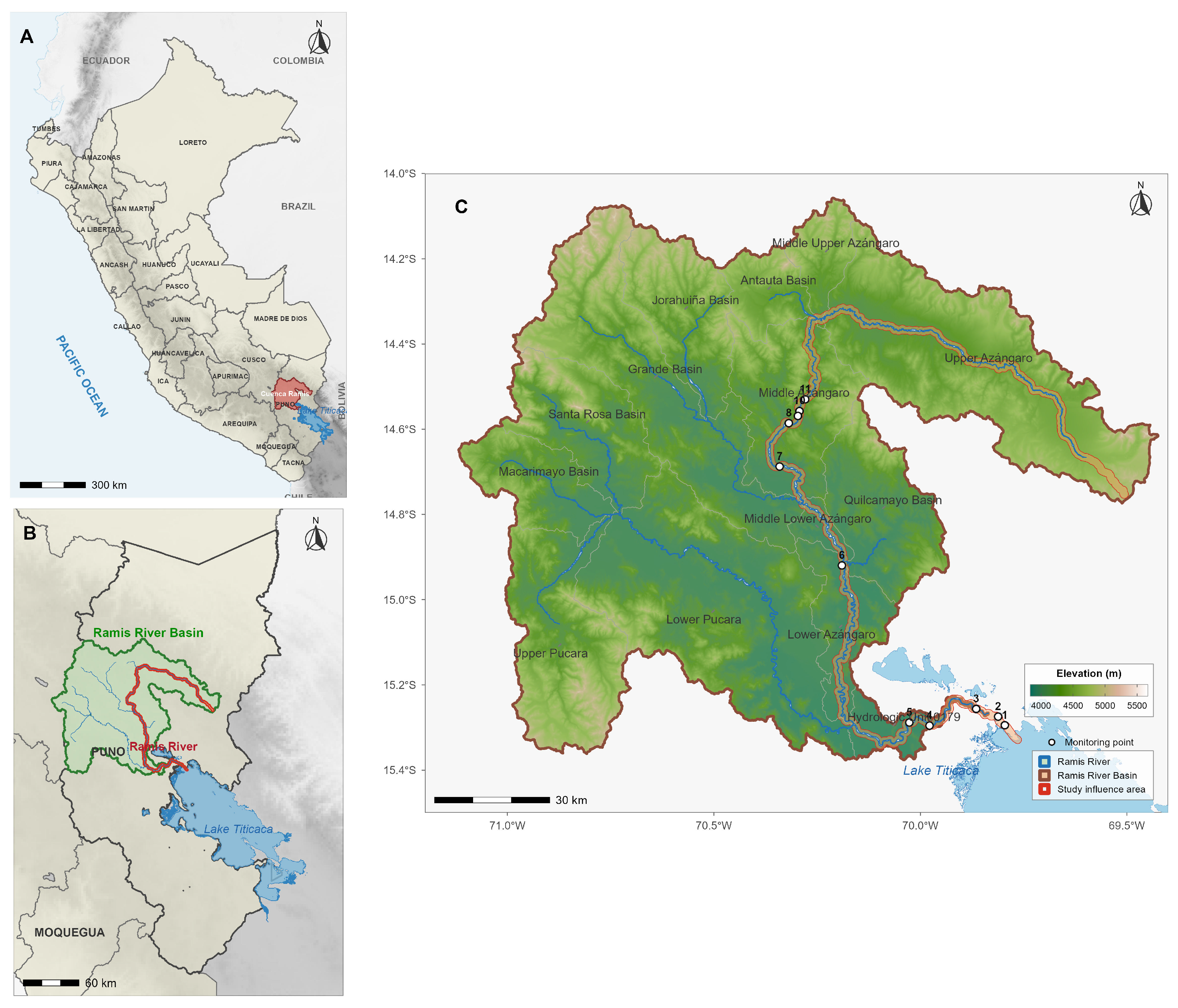
The Ramis River basin is located in the Puno region, geographically situated between the coordinates 71°07′4.7″ W and 69°25′26.4″ W longitude, and 15°27′33.7″ S and 14°03′26.6″ S latitude (Figure 1). Its highest point reaches 5750 m above sea level (Ananea Chico snow-capped mountain) and its lowest point is 3815 m.a.s.l., corresponding to Lake Titicaca. The basin is also considered one of the largest catchments feeding Lake Titicaca, with a total area of 14.706 km² and a perimeter of 982 km. The study area covers 358 km² and the total fluvial channel length is 370.02 km, with a mean channel gradient of 0.278% in the analyzed reach indicating a very gentle slope typical of lowland rivers or lower course river segments.

2.2. Analytical Procedures

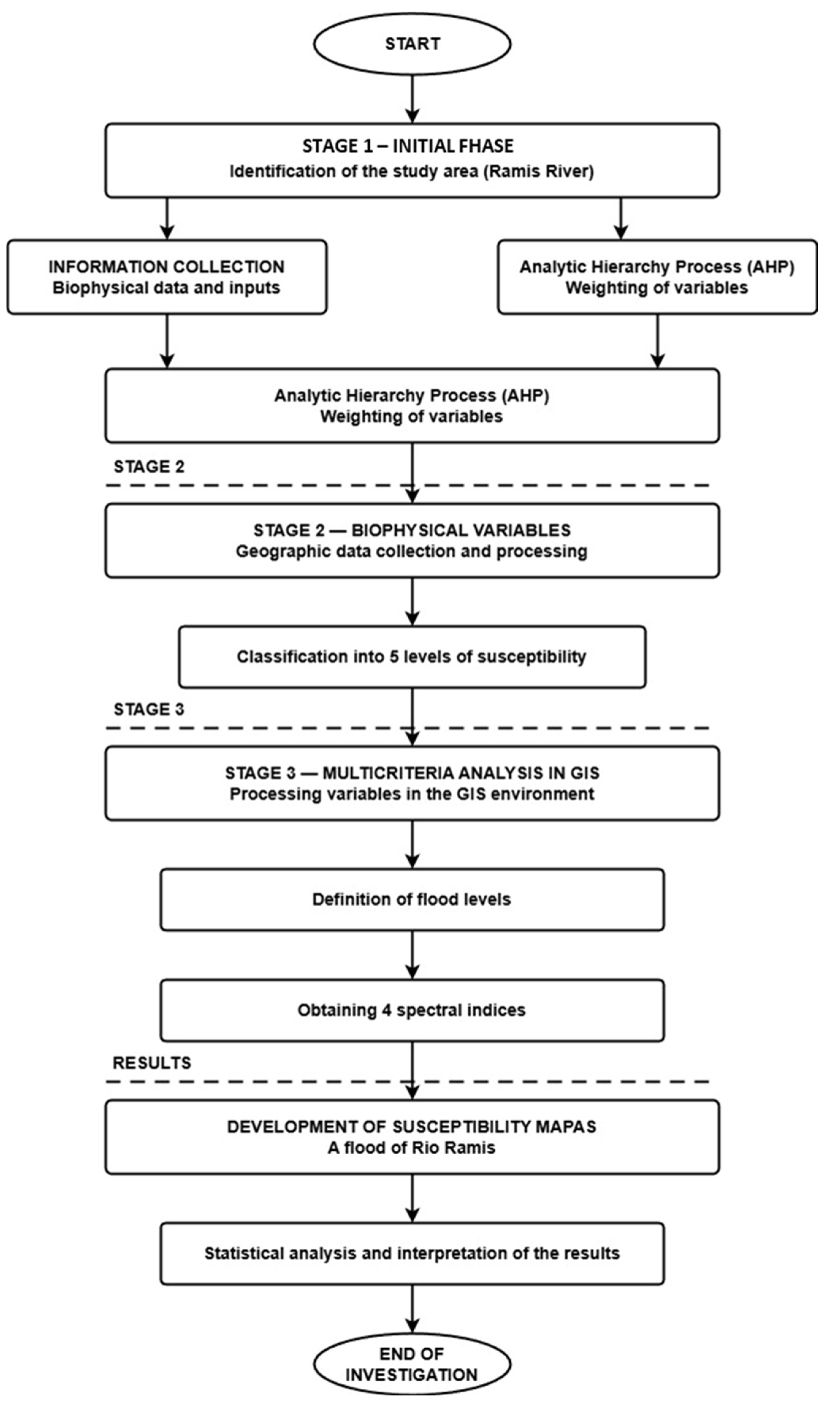
The characterization of zones susceptible to flooding along the Ramis River was carried out in four stages. The first, initial stage involved the identification of the study area; this was followed by a data collection phase conducted in parallel with the hierarchical analysis process and the analysis of flood susceptibility stratification levels. The second stage comprised the collection of biophysical variables with geospatial data processing, classifying them into five levels. The third stage involved variable processing through a multicriteria analysis within a GIS framework, the assignment of flood hazard levels, and the derivation of five spectral indices, culminating in the preparation of flood susceptibility maps, corresponding statistical analysis, and interpretation of results (Figure 2).

2.3. Geology, Geomorphology, Land Cover, Drainage Network, and Road Network

In this study, geomorphological and hydrological variables are the core foundation for analyzing flood dynamics and their regional distribution. Previous studies [25] note that geological and geomorphological features directly affect regional infiltration capacity, runoff formation processes, and flood propagation paths. For this reason, this study clarifies the source, processing method, and research value of each basic geographic variable one by one: Geological data are obtained from the GeoServer of Peru’s Ministry of Environment (MINAM), which can be used to identify regional lithological units, and then analyze their impacts on soil permeability and surface runoff. Geomorphological data are sourced from the ecological-economic zoning (ZEE) study of the Puno regional government, which can classify major topographic units such as alluvial plains, river terraces, and hillslopes. Existing studies have confirmed that these units are core factors affecting water accumulation and confluence during heavy rainfall events [26]. Land cover and land use analysis integrates vector ZEE data from MINAM, supplemented by visual interpretation results of Sentinel-2 satellite imagery. Relevant studies have verified that the multispectral characteristics of this imagery are suitable for land cover mapping [27].

During the analysis phase, topological correction was completed to eliminate layer overlaps, gaps, and geometric inconsistencies. Hydrological river network data are obtained from Peru’s National Geographic Institute (IGN), which is used to characterize the hydrological structure of the basin, and then extract the distance from river channels a flood susceptibility assessment predictor widely adopted in academic circles [28,29].

Finally, the road network distance layer is generated based on the national, regional, and local three-level road network provided by Peru’s Ministry of Transport and Communications (MTC). This variable is included because road accessibility is a core component of flood vulnerability, as it directly affects regional evacuation efficiency, emergency response capacity, and the connectivity of critical services. Existing studies have confirmed that flood damage to road networks will significantly reduce accessibility and increase the vulnerability of exposed populations [30,31,32].

2.4. Precipitation Data

The core monthly-scale precipitation data used in this study spans the period 1981–2021, and is sourced from the Peruvian climate-hydrology interpolation dataset PISCOp v2. This dataset is generated through interpolation of observational data from SENAMHI, Peru’s National Service of Meteorology and Hydrology. It features sufficient spatial coverage and strong record consistency, making it one of the highest-precision data sources for hydroclimatic analysis of the Peruvian Andes. The interannual variation in precipitation across the study area’s watersheds is significantly regulated by ENSO, and La Niña events generally increase the probability of flood occurrence in the southern Peruvian plateau; this conclusion is cited from reference [12].

2.5. Topographic Data and Terrain Slope

This study uses the 12.5-m-resolution ALOS PALSAR digital elevation model acquired from the Alaska Satellite Facility to derive slope and elevation values, and to identify flat areas and steep slopes. This resolution outperforms the 30-m SRTM data commonly used in regional research, and can accurately identify valley bottoms and microtopography that support flood dynamic research. This study divides slopes into four categories: flat terrain, which facilitates water accumulation; nearly flat terrain, which allows runoff to converge into depressions; moderately and gently undulating terrain, which supports relatively high flow velocities; and steep slopes, which are prone to rapid runoff and have high erosion potential.

2.6. Topographic Wetness Index (TWI)

This study uses the Topographic Wetness Index (TWI), combined with topographic morphology, to identify areas prone to water accumulation.

$$TWI=\ln \left({\displaystyle \frac{\mathsf{\alpha }}{\tan \mathsf{\beta }}}\right)$$

(1)

This index is calculated from a Digital Elevation Model (DEM) using Equation (1): in the formula, α is the upslope contributing area, and β is the local slope gradient. High TWI values correspond to confluence zones that are easily saturated and likely to cause disasters [4,9], and this index is a widely recognized core topographic predictor in flood susceptibility models [15].

2.7. Satellite Imagery and Spectral Index Derivation

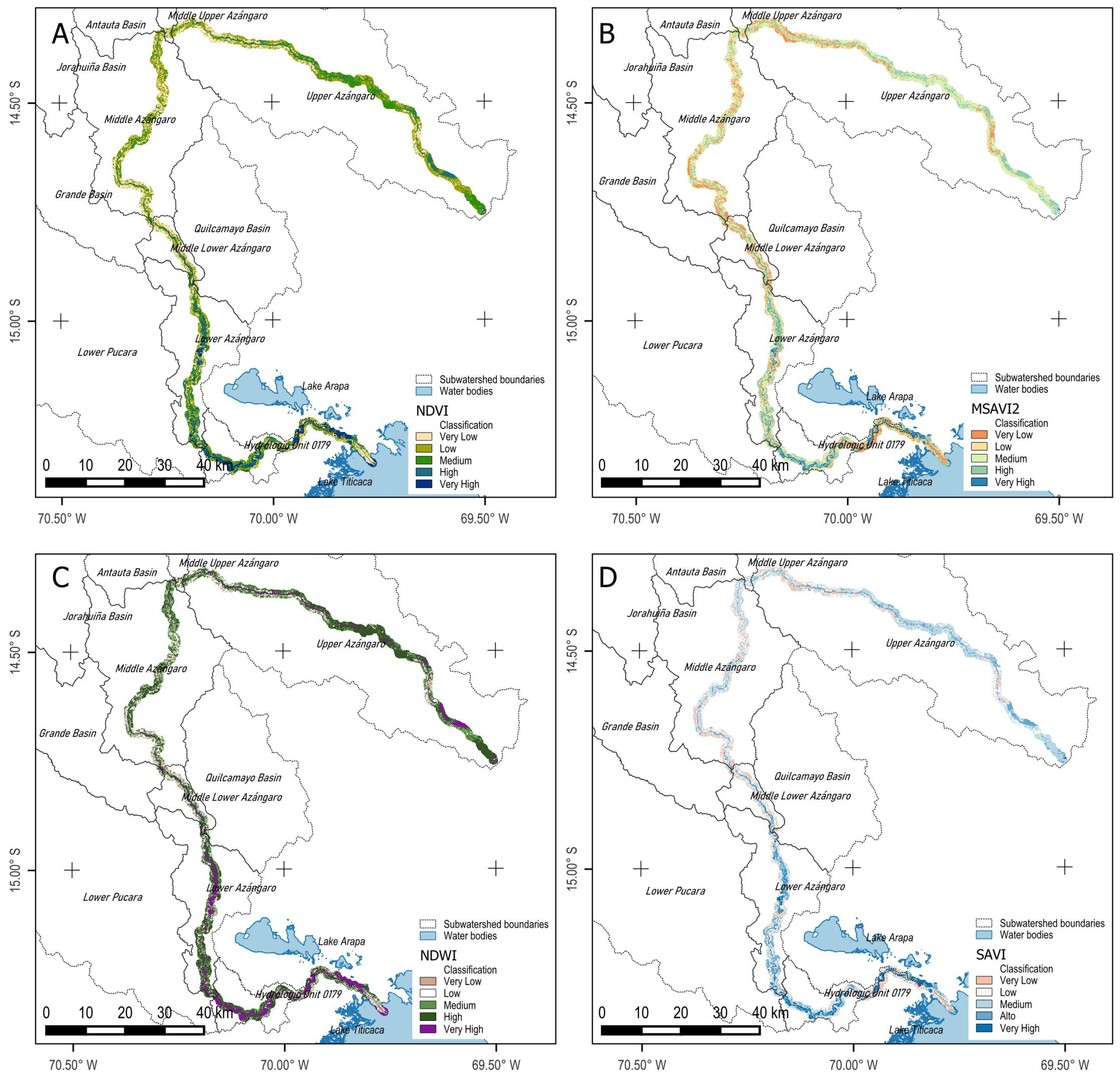
This study uses Planet satellite images obtained via the MIDAGRI platform in March 2025, with a spatial resolution of 4.5 m. It plans to calculate four types of spectral indices: NDVI (Normalized Difference Vegetation Index), NDWI (Normalized Difference Water Index), SAVI (Soil Adjusted Vegetation Index), and MSAVI2 (Modified Soil Adjusted Vegetation Index), following the approach recommended by [5], A total of 60 Planet satellite mosaics, including natural color (RGB) and near-infrared (NIR) imagery, were processed. The green (B4), red (B6), and near-infrared (B8) bands.

$$\mathrm{S}\mathrm{A}\mathrm{V}\mathrm{I} = {\displaystyle \frac{\left(\mathrm{N}\mathrm{I}\mathrm{R} - \mathrm{R}\mathrm{e}\mathrm{d}\right)}{\left(\mathrm{N}\mathrm{I}\mathrm{R} + \mathrm{R}\mathrm{e}\mathrm{d} + \mathrm{L}\right)}} \times \left(1 + \mathrm{L}\right)$$

(2)

$$NDWI={\displaystyle \frac{\left(Green-NIR\right)}{\left(Green+NIR\right)}}$$

(3)

$$NDVI={\displaystyle \frac{\left(NIR-Red\right)}{\left(NIR+Red\right)}}$$

(4)

$$MSAVI2={\displaystyle \frac{2\times NIR+1-\sqrt{{\left(2\times NIR+1\right)}^2-8\times \left(NIR-Red\right)}}{2}}$$

(5)

2.8. Multicriteria Analysis Framework

The multicriteria analysis for determining hazard levels was conducted using the Analytic Hierarchy Process (AHP), applying the pairwise comparison model proposed by [33]. This method was selected for its capacity to integrate expert judgment with quantitative data within a structured and reproducible framework, and has been widely applied in flood susceptibility studies [15,16,25]. The methodology comprised the evaluation of eight criteria: geomorphology, geology, terrain slope, precipitation, Vegetation cover, the Topographic Wetness Index (TWI), drainage network, and road network. The relative importance of these criteria was determined using an 8 × 8 pairwise comparison matrix developed from a systematic literature review and expert consultation (

Table 1. Pairwise comparison matrix of the evaluation criteria using the Analytic Hierarchy Process (AHP).

Criteria	Geomorphology	Geology	Slope	Precipitation	Vegetation Cover	TWI	Drainage Network	Road Network
Geomorphology	1	3	4	5	6	7	8	9
Geology	1/3	1	3	4	5	6	7	8
Slope	1/4	1/3	1	3	4	5	6	7
Precipitation	1/5	1/4	1/3	1	2	4	5	6
Vegetation cover	1/6	1/5	1/4	1/2	1	3	4	5
TWI	1/7	1/6	1/5	1/4	1/3	1	2	4
Drainage network	1/8	1/7	1/6	1/5	1/4	1/2	1	3
Road network distance	1/9	1/8	1/7	1/6	1/5	1/4	1/3	1

).

The weight of each criterion is obtained from the principal eigenvector of the pairwise comparison matrix. The consistency of the judgments is evaluated using (Equations (6) and (7)):

$$CI={\displaystyle \frac{{\lambda }_{max}-n}{n-1}}$$

(6)

$$CR={\displaystyle \frac{CI}{RI}}$$

(7)

where λmax is the maximum eigenvalue, n is the number of criteria, CI is the consistency index, RI is the random index, and CR is the consistency ratio.

A CR value of <0.10 is considered acceptable. This ensures that the pairwise comparisons are logically consistent and that the derived weights are methodologically reliable for constructing the final susceptibility map.

The maximum eigenvalue of the pairwise comparison matrix was λmax = 8.76, resulting in a Consistency Index (CI) of 0.109. The normalized priority vector indicated that geomorphology was the most influential criterion, with a weight of 0.35, followed by geology (0.23) and terrain slope (0.15). Together, these three factors accounted for 73% of the total weight assigned in the multicriteria model (

Table 2. Pairwise ranking to determine the risk level.

Code	Factor	Type	Description	Weight
FC1	Geomorphology	Conditioning	Controls flow accumulation and direction	0.35
FC2	Geology	Conditioning	Influences infiltration and permeability	0.23
FC3	Slope	Conditioning	Determines runoff velocity	0.15
FD	Precipitation	Triggering	Primary flood-triggering factor	0.10
FC4	Vegetation cover	Conditioning	Reduces surface runoff	0.07
FC5	TWI	Conditioning	Topographic wetness index	0.04
FC6	Drainage network	Conditioning	Facilitates flow concentration	0.03
FC7	Road network distance	Conditioning	Modifies natural drainage patterns	0.02

). The consistency of the pairwise judgments was evaluated using the Consistency Ratio (CR), calculated as CI/RI, where the Random Index for an 8 × 8 matrix was RI = 1.404. The resulting CR was 0.078. Since this value was below the commonly accepted threshold of 0.10, the comparison matrix was considered sufficiently consistent, supporting the reliability of the derived factor weights (

Table 3. Consistency evaluation of the AHP pairwise comparison matrix.

Parameter	Value
Number of criteria	8
Λmax	8.76
Consistency Index (CI)	0.109
Random Index (RI)	1.41
Consistency Ratio (CR)	0.078
Decision	Acceptable (CR < 0.10)

).

Flood susceptibility (S) was calculated through the weighted combination of flood-conditioning factors, following the methodology proposed by the National Center for Disaster Risk Estimation, Prevention and Reduction [34], as expressed in Equation (8):

$${\mathrm{S}=\mathrm{F}\mathrm{C}}_{W_{FC}}+{\mathrm{F}\mathrm{D}}_{W_{FD}}$$

(8)

where FC is the normalized index of conditioning factors and FD is normalized precipitation. The weights satisfy ${\mathrm{w}}_{\mathrm{F}\mathrm{C}}$ + ${\mathrm{w}}_{\mathrm{F}\mathrm{D}}$ = 1, with ${\mathrm{w}}_{\mathrm{F}\mathrm{C}}$ = 0.4 and ${\mathrm{w}}_{\mathrm{F}\mathrm{D}}$ = 0.60. Since ${\mathrm{w}}_{\mathrm{F}\mathrm{D}}$ > ${\mathrm{w}}_{\mathrm{F}\mathrm{C}}$, precipitation has a greater contribution to susceptibility, reflecting its role as the primary triggering mechanism for flooding.

The final flood hazard index (R) (9) was estimated by integrating the susceptibility index (S) with the normalized hydrological parameter representing the precipitation return period (PE):

$$\mathrm{R}=S_{W_S}+{PE}_{W_{PE}}$$

(9)

With ${\mathrm{w}}_{\mathrm{S}}$ + ${\mathrm{w}}_{\mathrm{P}\mathrm{E}}$ = 1, where ${\mathrm{w}}_{\mathrm{S}}$ = 0.60 and ${\mathrm{w}}_{\mathrm{P}\mathrm{E}}$ = 0.40. Thus, the susceptibility index contributes 1.5 times more to the final hazard index than the return-period parameter, in accordance with the adopted weighting scheme.

The return period was classified into five categories: 2, 5, 10, 25, and 50 years. The resulting hazard levels and their corresponding ranges are presented in

Table 4. Flood hazard level and risk-range classification.

Hazard Level	Range
Very low	R ≤ 0.035
Low	0.035 ≤ R < 0.073
Moderate	0.073 ≤ R < 0.132
High	0.132 ≤ R < 0.268
Very high	1.268 ≤ R ≤ 0.468

Note: Colors indicate increasing flood hazard severity from very low (green) to very high (red).

. In this table, PE denotes the normalized index associated with the precipitation return period.

2.9. Geospatial Data Processing—Geoprocessing

Spatial data processing was initially performed by handling vector information corresponding to the seven conditioning factors. Polyline-format information was transformed into influence areas using Euclidean distances. Subsequently, each vector information class was reclassified into five levels based on flood susceptibility.

This information was then incorporated into the Weighted Overlay tool in ArcGIS version 10.8.2. Finally, flood hazard levels and ranges were integrated to generate the final composite analysis.

2.10. Independent Validation Through Field Expeditions

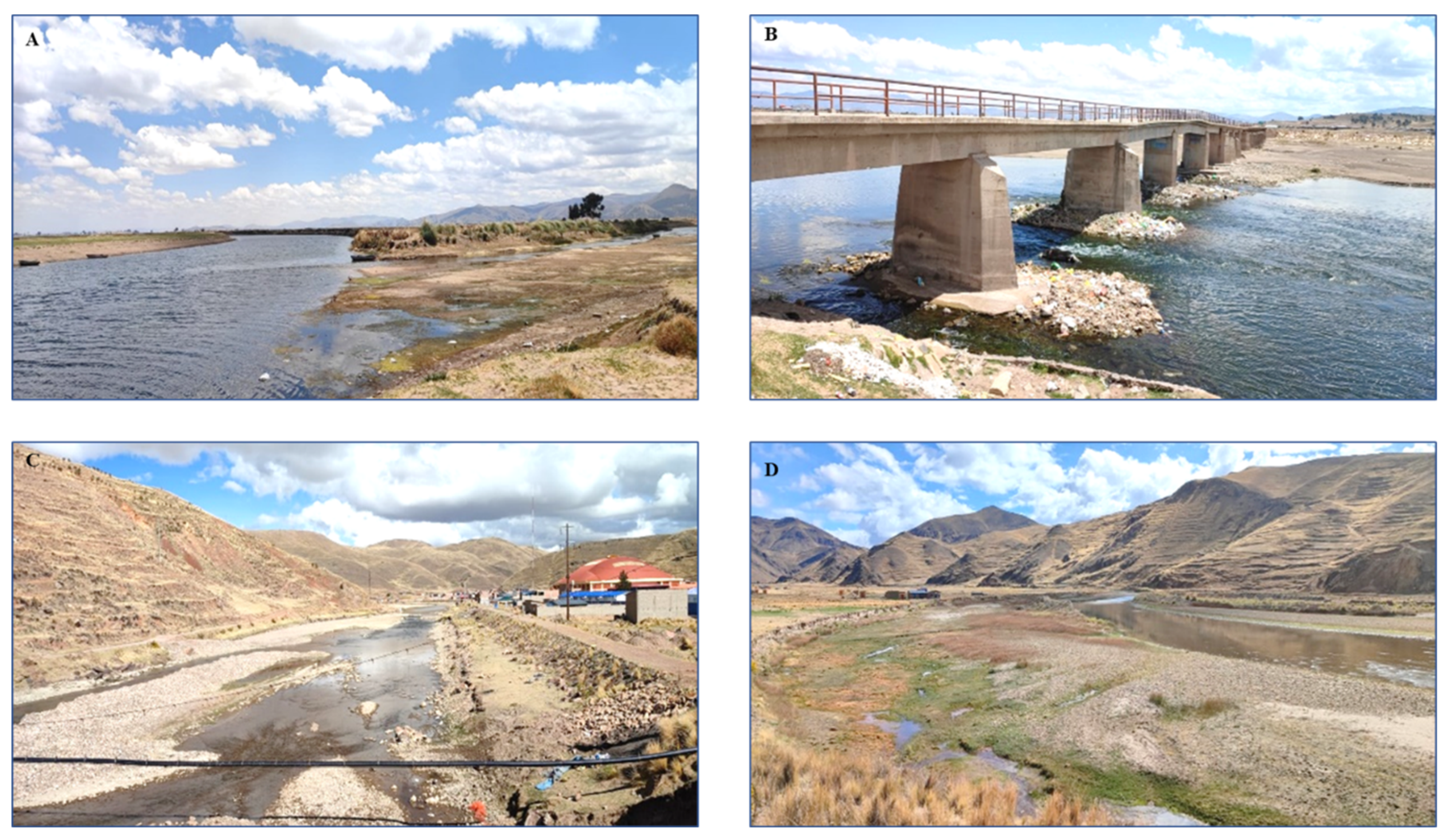
Field expeditions were conducted in December 2023 to independently validate the hazard maps and assess flood-prone areas along critical reaches of the Ramis River hydrographic network. The model outputs were compared with empirical field observations collected at 11 independent validation points. Figure 3A shows the confluence of the Ramis and Huancané rivers, characterized by minimum discharge conditions. Figure 3C depicts the bridge located in the Taraco district, representing a confined river reach with protection structures. Figure 3C presents the San Antón bridge, where riparian protection zones were identified. Finally, Figure 3D illustrates the sector between Toncuri and Hacienda Triunfo, where agricultural areas affected by overflow and flooding were documented.

2.11. Statistical Validation

Statistical validation of the flood susceptibility map was conducted using R 4.3.3 + RStudio 2024.02.0+443, using four spectral indices derived from satellite imagery: NDVI (Normalized Difference Vegetation Index), NDWI (Normalized Difference Water Index), SAVI (Soil Adjusted Vegetation Index) and MSAVI2 (Modified Soil Adjusted Vegetation Index). All raster data were spatially homogenized through reprojection and nearest-neighbor resampling. A random spatial sample of 1484 valid pixels was extracted for statistical and geostatistical analysis.

Relationships between spectral indices and flood susceptibility were evaluated through: (i) Spearman correlation (Equation (10)), (ii) Global Moran’s spatial autocorrelation (Equation (11)), (iii) Bivariate Moran’s Index (Equation (12)), and Complementarily, a Random Forest modeling was implemented to classify flooded and non-flooded zones [35] (Equation (13)). The dependent variable was binarized, considering classes 4 and 5 as flood-prone zones and classes 1–3 as non-flooded areas. The model was validated using a confusion matrix, Accuracy, Kappa, Sensitivity, Specificity, and the Area Under the ROC Curve (AUC). This approach is consistent with best practices reported in the recent literature for susceptibility model validation [4,18].

$${\rho }_s=1-{\displaystyle \frac{6\sum d_i^2}{n\left(n^2-1\right)}}$$

(10)

where $d_i$ is the difference between the ranks of each pair of observations, and n is the total number of observations.

$$I={\displaystyle \frac{n}{S_0}}{\displaystyle \frac{\sum \sum w_{ij}\left(x_i-\overline{x}\right)\left(x_j-\overline{x}\right)}{\sum {\left(x_i-\overline{x}\right)}^2}}$$

(11)

$$I_{xy}={\displaystyle \frac{n}{S_0}}{\displaystyle \frac{\sum \sum w_{ij}\left(x_i-\overline{x}\right)\left(y_j-\overline{y}\right)}{\sqrt{\sum {\left(x_i-\overline{x}\right)}^{2\sum {\left(y_j-\overline{y}\right)}^2}}}}$$

(12)

where n is the number of spatial units, $w_{ij}$ is the spatial weight matrix, $S_0$ is the sum of the weights, $x_i$, y, $x_j$ are the observed values, and $\overline{x}$ is the overall mean.

$$\widehat{P}\left(y=c∣x\right)={\displaystyle \frac{1}{T}}\sum I\left(h_t\left(x\right)=c\right)$$

(13)

where $\widehat{P}\left(y=c∣x\right)$ is the estimated probability that the sample x belongs to class c; T is the total number of trees in the forest; $h_t$(x) represents the prediction of tree t; and I(⋅) is an indicator function that assigns the value 1 when the prediction matches the evaluated class and 0 otherwise.

3. Results

3.1. AHP-Derived Weights and Key Factors Controlling Flood Hazard

The AHP analysis established the relative importance of the selected variables within the flood susceptibility index. Geomorphology obtained the highest weight (0.35), followed by geology (0.23) and terrain slope (0.15), indicating their dominant contribution to the multicriteria model. Together, these three factors accounted for 73% of the total weight, representing the main determinants of spatial flood susceptibility. Precipitation showed a weight of 0.10, confirming its role as the main triggering factor in the flood assessment. The TWI (0.07) and land cover (0.04) presented intermediate contributions, while drainage network (0.03) and road network distance (0.02) exhibited lower weights within the model.

The consistency evaluation of the AHP matrix showed a Consistency Ratio (CR) of 0.078, which is below the acceptable threshold of 0.10. This indicates that the pairwise comparisons were consistent and that the derived weights are reliable for integration into the flood susceptibility and hazard models.

These results are consistent with the specialized literature that ref. [15] identified river proximity as the most significant criterion, followed by precipitation and land use. Ref. [16] highlighted geomorphology as the primary factor in multicriteria studies in East Africa. Ref. [3] incorporated drainage density and road distance. Ref. [36] confirmed the relevance of AHP for integrating heterogeneous criteria in the assessment of vulnerability to extreme events. The methodological consistency across these studies validates the approach employed in the Ramis basin.

3.2. Quantitative Establishment of Susceptibility Classes

The AHP-based multicriteria analysis integrated into the GIS framework classified the Ramis River basin into five flood susceptibility classes.

Table 5. Quantification of flood susceptibility levels in the Ramis River basin.

Class	Range	Area (km2)	Percentage (%)
High	0.132–0.268	22.08	6.2
Low	0.035–0.073	55.25	15.4
Moderate	0.073–0.132	236.54	66.0
Very high	0.268–0.468	44.12	12.3
Very low	<0.035	0.49	0.14
Total		358	100

shows the spatial distribution of the five flood hazard classes in the Ramis River basin. The moderate hazard class covered the largest area, at 236.54 km² (66.0%), followed by the low hazard class, at 55.25 km² (15.4%), and the very high hazard class, at 44.12 km² (12.3%). Meanwhile, the high and very low hazard classes covered 22.08 km² (6.2%) and 0.49 km² (0.14%), respectively. Taken together, these results indicate a predominance of moderate hazard conditions in the basin, while the high and very high categories represent a smaller but spatially significant proportion of the total area of 358 km².

Figure 4 shows the spatial distribution of flood hazard across six sectors of the Ramis River basin: (A) Upper Azángaro; (B) the middle sector of the Upper Azángaro sub-basin; (C) the sector between the Upper Azángaro–Antauta and Middle Azángaro sub-basins; (D) the sector from Middle Azángaro to Middle-Lower Azángaro; (E) the sector from Middle-Lower Azángaro to Lower Azángaro; and (F) the sector from Lower Azángaro to Hydrographic Unit 0179, which flows into Lake Titicaca. The spatial distribution shows a higher concentration of the high and very high hazard categories in areas near the main channel and its major tributaries, while the low and very low categories predominate on slopes and in areas with less direct influence from watercourses.

These results are consistent with findings from comparable studies in Andean and tropical basins [15], in a multicriteria study of the Kathmandu basin (Nepal), reported that 56% of the area exhibited moderate flood susceptibility a pattern similar to that observed in the Ramis [9], in the Subarnarekha basin (India), confirmed the dominance of moderate risk zones in high-mountain fluvial systems with marked climatic variability. In the Peruvian Andean context, ref. [19] emphasized the importance of climatic variability and land use on the Ramis hydrological regime, consistent with the factors identified in this study as determinants of predominant moderate risk.

Through refined spatial analysis, this paper finds that natural flat river channel areas have a high flood susceptibility, which is linked to stable erosion and the accumulation of loose sediments in these regions. In contrast, steep slopes with high vegetation coverage are barely affected by the river network and have low flood susceptibility. The conclusion that vegetation can reduce flood susceptibility has been widely verified in references [4,17].

3.3. Geospatial Results of Spectral Indices

Our team selected Planet satellite images captured during the 2025 March flood season of the Ramis River. We extracted four types of spectral indices, and divided each index into five susceptibility levels. Calculations showed that the estimated flood areas derived from indices such as SAVI = 38.29 km² (Figure 5A), MSAVI2 = 36.73 km² (Figure 5B), NDWI = 101.87 km² (Figure 5C) and NDVI = 39.75 km² (Figure 5D) differed significantly. These differences were not caused by methodological errors, but instead stemmed from the varying spectral sensitivity of each index to environmental factors including water bodies and sediments.

3.4. Statistical Validation of Spectral Indices and Flood Susceptibility Zones

The Spearman analysis in this study (

Table 6. Spearman Correlation, Global Moran’s Index, and Bivariate Moran’s Index.

Index	Spearman (ρ)	Moran’s I	p-Value	Bivariate Moran’s
NDVI	−0.2526	0.2850	<0.001	−0.1114
NDWI	−0.2487	0.2513	<0.001	−0.0566
SAVI	−0.2395	0.2161	<0.001	−0.0529
MSAVI2	−0.22	0.2119	<0.001	−0.0124

Note: Analyses were performed using 1484 spatial samples.

) shows that spectral indices are negatively correlated with flood susceptibility. The results for NDVI (ρ = −0.2526), NDWI (ρ = −0.2487), SAVI (ρ = −0.2395), and MSAVI2 (ρ = −0.22) are consistent with the conclusions of references [37,38].

The global spatial autocorrelation analysis results of this study show that the Moran’s I indices of all spectral indices are positive and statistically significant (p < 0.001). Among them, the Normalized Difference Vegetation Index (NDVI) has the highest level of spatial clustering, with an I value of 0.2850. This leads to the inference that all spectral variables exhibit a structured, non-random spatial distribution that is strongly tied to flood-prone and non-flood-prone zones. Subsequent bivariate Moran’s I analysis yielded negative results, confirming that flood sensitivity and vegetation activity have an inverse spatial dependence. NDVI is the spectral predictor with the strongest spatial robustness for identifying high-risk areas.

Existing studies support the rationality of this conclusion: a study of a watershed in southern Brazil [8], verified that NDVI and the Normalized Difference Water Index (NDWI) can distinguish active flood zones from potential flood zones, and another study [18] proposed that combining spectral indices with spatial autocorrelation analysis can significantly improve the detection accuracy of hydrological patterns in watersheds with scarce data.

The prediction performance of the random forest model used in this study is as follows: AUC = 0.6935, overall accuracy of 63.51% (

Table 7. Random Forest model validation metrics.

Metric	Value
AUC	0.6935
Accuracy	0.6351
Kappa	0.2565
Sensitivity	0.5978
Specificity	0.6615

Note: Based on 1484 spatial samples, statistical, spatial autocorrelation, and Random Forest validation analyses were conducted.

), sensitivity of 0.5978 (which enables effective identification of flood-prone areas), and specificity of 0.6615 (which enables correct discrimination of non-flood areas). The Kappa coefficient is 0.2565, meaning the consistency between observed and predicted classifications meets the required standard.

4. Discussion

This study finds that flood susceptibility in the study area is driven by the complex interactions of eight factors: geomorphology, geology, slope, topographic wetness index, vegetation coverage, river network, distance from roads, and precipitation. Against this backdrop, the relatively high weight of 0.35 assigned to the geomorphology factor in this study is fully reasonable. This assignment is consistent with the conclusions of existing literature. The geomorphology factor can not only reflect topographic morphology, but also integrate information on floodplains, river terraces, depressions, and flow concentration corridors, covering the surface’s capacity to store, transport, and accumulate runoff. References [39,40] also note that machine learning methods incorporating explicit geomorphological variables produce more accurate representations of the spatial structure of flood disasters and achieve better performance. Therefore, this weight assignment is by no means arbitrary; it is a direct reflection of the factor’s ability to accurately capture topographic conditions related to water accumulation and flow concentration.

To understand the core value of geomorphology in flood susceptibility models, one must examine research on the performance of flood prediction models. Existing studies show that Reference [39] found that the random forest model performs well in simulating low-to-moderate magnitude flood discharges, but its performance declines for extreme flood events, and this model is sensitive to the types of available hydrological data. Similarly, reference [40] proposed that when sufficient information is available, random forests can predict flood water levels with high accuracy, but their performance always depends on the ability of predictive variables to capture the actual dynamics of the system. Building on these two findings, in the complex Andean landscape where topographic and valley morphology dominate hydrological processes, geomorphology plays a structural supporting role in flood susceptibility models.

The performance of the Random Forest model, with an overall accuracy of 69%, should be interpreted as an acceptable result but one that is still limited by the complexity of the phenomenon under study. Although Random Forest is widely recognized for its robustness in the face of nonlinear relationships and its ability to handle interactions among variables, its accuracy may decrease when the system exhibits high spatial heterogeneity or when dynamic variables directly linked to the flood event are missing. Ref. [39] noted that, even in large-scale flow simulations, the model struggles to adequately reproduce larger-scale events, especially in basins where climatic and altitudinal structure introduces additional variability. More recent studies have shown that incorporating variables derived from remote sensing, spectral indices, and hydrodynamic characteristics improves predictions but does not completely eliminate the uncertainty associated with the spatial and temporal scale of the analysis [40]. Therefore, the level of accuracy achieved can be considered reasonable as a first cartographic approximation, although it also highlights the need to incorporate more direct hydrometeorological variables, field data, and higher-resolution data to improve predictive capability [41].

In the case of the NDWI, the observed overestimation of water compared to other indices is consistent with its known spectral limitations. Ref. [42] showed that the classic NDWI tends to include noise from non-aquatic surfaces, particularly in environments with urban backgrounds, bare soil, or areas with intense spectral mixing; it also remains sensitive to wet pixels, waterlogged surfaces, and water-saturated vegetation. This explains why, in heterogeneous landscapes with shallow flooding, the index may classify areas as water that actually correspond to saturated soil or very wet vegetation cover. Studies conducted in high-Andean wetlands also show that water indices should be interpreted with caution, as their behavior can vary depending on the time of year, the type of land cover, and the spatial resolution of the image used [42,43]. Consequently, the NDWI detects not only open water but also surface moisture conditions that may overestimate the actual extent of flooding.

The negative correlations observed between NDVI/SAVI and flood susceptibility are consistent with the effects of prolonged waterlogging, which may reduce vegetation vigor through root hypoxia, substrate instability, and altered sedimentation processes. However, this relationship is not universal in high-Andean ecosystems, where water availability can support dense and productive vegetation. In bofedales, water is seasonally stored and gradually released, contributing to dry-season baseflow and ecosystem productivity. Therefore, abundant water may coexist with high NDVI values during certain seasons, depending on hydrological conditions, vegetation type, and climate variability [43,44,45].

This point is particularly important because it prevents an overly simplified interpretation of the relationship between vegetation indices and susceptibility. In systems where flooding leads to degradation or loss of vegetation cover, the negative relationship between NDVI/SAVI and susceptibility is logical. However, in high-Andean bofedales and wetlands, moisture may be precisely the factor that allows dense and functional vegetation to persist. Therefore, the sign of the correlation depends on whether the analyzed area corresponds to a zone of destructive flooding, a permanent wetland, or a transitional matrix between these two states. In this regard, the literature on bofedales emphasizes that their structure and dynamics are strongly linked to water regulation, the seasonality of precipitation, and interannual climate variability, which necessitates a cautious interpretation of spectral indices when they are used as proxies for flood susceptibility [43].

The moderate AUC values obtained are explained by the limitations of using spectral indices as the sole model predictors: these capture surface conditions at specific moments but do not directly integrate dynamic variables such as streamflow or the historical frequency of flooding. Reference studies such as [4] which incorporated 13 geospatial inputs with XGBoost and CatBoost models in an arid-urban context, achieved AUC values of 0.92 [18] reported AUC of 0.873 using 9 variables. The difference is explained by the greater complexity of the variable sets and the availability of more complete historical flood inventories. In Andean basins with scarce data, results comparable to those obtained in this study (AUC ≈ 0.70) are reported as acceptable in the specialized literature.

The SHAP analysis applied in methodologically advanced studies such as [4] constitutes a potential improvement for future studies in the Ramis basin, enabling identification of the marginal contribution of each spectral variable to the predictive model and increasing the scientific interpretability of results. The future incorporation of SAR data (Sentinel-1) for the generation of historical flood inventories would substantially improve the machine learning model’s performance, as documented by [46] and susceptibility studies with SAR data in tropical basins.

Theoretical and Practical Implications

This study integrates multi-criteria analysis with GIS technology to address the complex challenge of hydrological risk in Andean River basins, representing a major breakthrough in this field. On the theoretical level, this study advances understanding of the interactions among geomorphic, climatic, and anthropogenic processes in research on flood susceptibility under the context of high hydrological variability and climate change. It identifies geomorphology and geology as the dominant factors driving flood susceptibility: the lithological base and topographic configuration constrain hydrological responses at a structural level, which can consolidate the theoretical foundation of mountain basin hydrology.

On the practical level, the susceptibility maps generated in this study can serve as a core input for four key types of work: planning for protection and disaster reduction engineering in high-susceptibility areas, spatial planning and land-use regulation in risk zones, design of early warning systems adapted to spatially differentiated precipitation thresholds, and adaptive strategies to enhance the resilience of riparian communities [14,20,21]. This set of methods can also be replicated in other Andean basins with similar characteristics to expand its regional influence [23].

Continuous monitoring of spectral indices and periodic updating of susceptibility maps, integrated with projected climate data under climate change scenarios, will enable the assessment of the temporal evolution of flood risk in the Ramis basin. Coordination with risk management platforms of Peru’s National Civil Defense Institute (INDECI) and the National Center for Estimation, Prevention, and Reduction of Disaster Risk (CENEPRED) would ensure effective knowledge transfer to decision-makers at the regional and local levels.

5. Conclusions

This study provides a robust geospatial assessment of flood susceptibility in the Ramis River basin, identifying geomorphology and geology as the primary determining factors, followed by land slope and precipitation. This classification, obtained using the Analytic Hierarchy Process (AHP) and supported by a systematic literature review and expert consultations, is consistent with previous studies conducted in Andean and tropical watersheds.

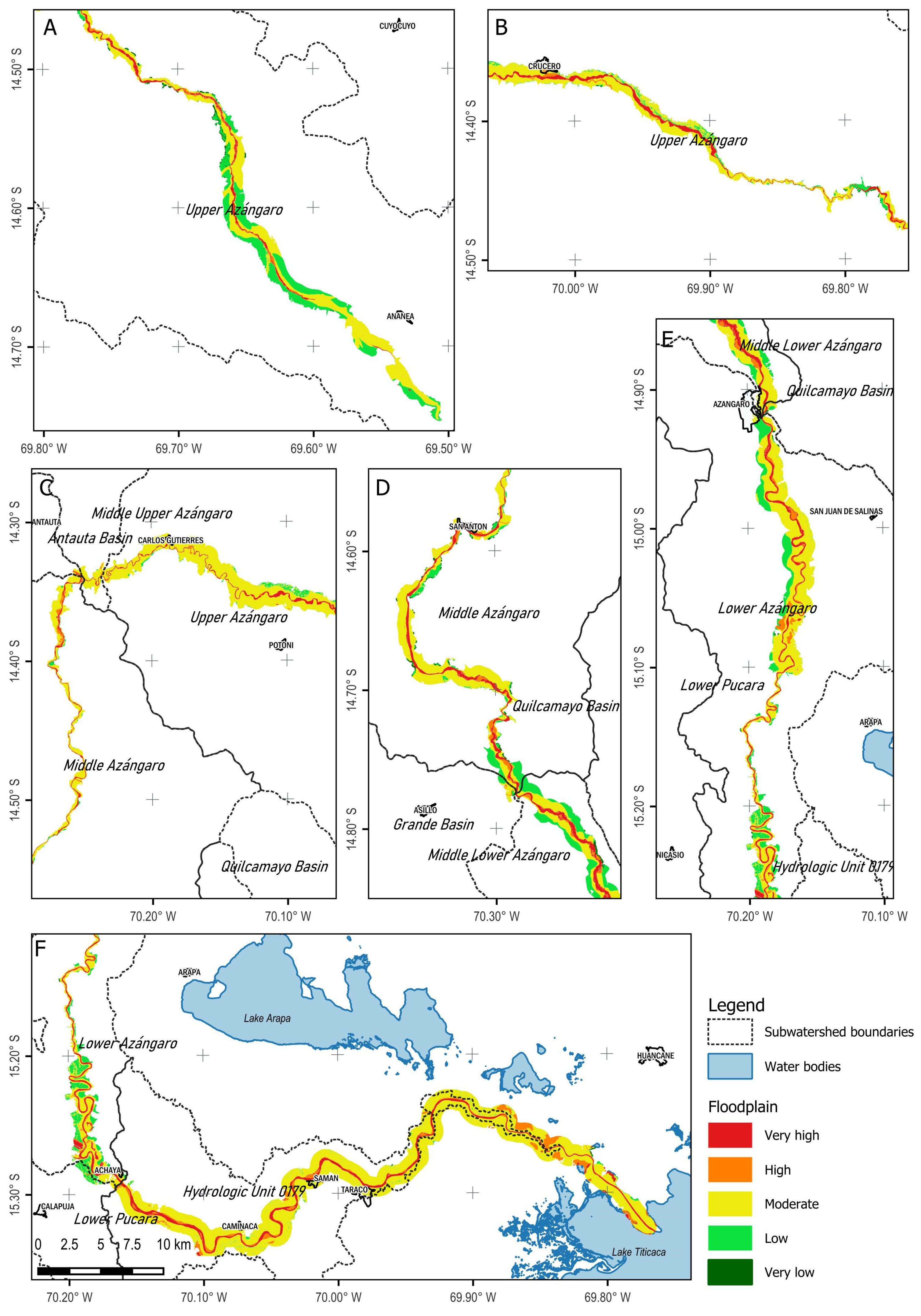
This study conducts a core review of the watershed flood risk assessment field and advances its research outputs through three research modules. First, it applies the AHP-GIS multi-criteria classification method to identify five flood sensitivity levels. Among these, the moderate-risk level accounts for the largest share at 66%, corresponding to an area of 236.54 km².

It is followed by the extremely high-risk zone, which accounts for 12.3% and covers 44.12 km², and the high-risk zone, which accounts for 6.2% and covers 22.08 km². This distribution confirms that flood risks in the watershed have spatial heterogeneity, which requires differentiated environmental management strategies, and completes the anchoring of the research background. Next, the study compares the flood extent estimation results of four types of spectral indices. The estimated values of these four indices range from 36.73 km² to 101.87 km², showing significant differences. These differences stem from the varying response sensitivities of each index to surface water, sediment deposition, soil moisture, and vegetation, rather than flaws in the methods. Among the indices, the NDWI produces an estimated value of 101.87 km², which can effectively capture overall moisture and sediment traces, but it tends to overestimate inundation area in active sedimentary environments.

The NDVI produces an estimated value of 39.75 km², which can more accurately delineate severely vegetation-damaged areas related to floods. This leads to the conclusion that a single spectral index cannot fully describe flood dynamics, and complementary remote sensing indicators must be integrated to improve the reliability of assessments. Finally, the study completes statistical verification using Spearman correlation, global Moran’s index, and bivariate Moran’s index. The results confirm that there is a significant spatial correlation between flood risk maps and the extracted spectral indices, and all indices show significant spatial autocorrelation (p < 0.001). Among them, NDVI has the strongest negative correlation (ρ = −0.2526) and the highest spatial autocorrelation (Moran’s I = 0.2850), making it suitable for identifying vegetation degradation in flood zones. The random forest model has moderate classification performance (AUC = 0.6935, accuracy = 63.51%), which indicates that the spatial patterns captured by the spectral indices are consistent with flood risks. Adding additional environmental variables and multi-temporal datasets can further improve the model’s performance. In the future, integrating Sentinel-1 SAR data with interpretable artificial intelligence technologies such as SHAP can enhance the robustness and interpretability of assessments.