Evaporative Water Consumption and Heat Redistribution Under Pumped-Storage Hydropower Operation in an Arid Region

Abstract

Pumped-storage hydropower (PSH) can modify reservoir evaporation in arid regions by altering water-level dynamics, surface-area exposure, and thermal exchange between reservoirs. This study quantifies operation-induced evaporation changes at the Fukang PSH station in Xinjiang, China, using a one-dimensional lumped hydrodynamic–thermal model driven by hourly station observations and ERA5 reanalysis for 2024. A four-scenario factorial design separates thermal, surface-area, and interaction effects within a unified water energy framework. Under station forcing, fully coupled operation reduces annual system-scale evaporation from 135.36 × 10⁴ m³ to 115.45 × 10⁴ m³, corresponding to a net reduction of 19.91 × 10⁴ m³ (14.7%). Energy-budget analysis identifies advective heat transport as the main pathway linking dispatch, reservoir thermal evolution, and evaporation response, with annual cumulative values of +205 TJ in the upper reservoir and −333 TJ in the lower reservoir. Dispatch-regime experiments further show that stronger exchange-flow operation does not necessarily increase evaporation reduction: the low, baseline, and enhanced schedules produce system-scale net changes of 37.70 × 10⁴ m³, 19.91 × 10⁴ m³, and −3.41 × 10⁴ m³, respectively. These results indicate that evaporation effects in arid-region PSH systems depend on the timing of surface-area exposure relative to local evaporative demand, rather than on exchange-flow magnitude or operating duration alone.

1. Introduction

Pumped-storage hydropower (PSH) supports renewable-energy integration by providing large-scale storage and flexible regulation [1,2]. Previous work has also highlighted its seasonal storage and water-storage potential [3,4]. Its hydrological effects, however, require separate assessment because repeated pumping and generation alter reservoir water levels, exchange flows, and thermal conditions. These operational changes can modify open-water evaporation, especially where water availability constrains hydropower development and water-resource allocation.

In arid and semi-arid regions, evaporation from hydraulic infrastructure forms part of the regional water-resource balance rather than a purely local surface-water process. PSH operation may disturb reservoir thermal regimes and ecological conditions [5,6], while climate change and reservoir evaporation can further alter water availability in dryland basins [7,8]. Broader hydroclimatic assessments also show that terrestrial water storage and arid-region water availability vary substantially across regions [9,10]. Recent studies indicate that PSH systems have clear value for energy-system flexibility [11], which makes it necessary to evaluate their water-consumption effects together with their energy benefits.

Open-water evaporation has been estimated using energy-balance and aerodynamic approaches for natural lakes and conventional reservoirs [12,13]. Combination-equation formulations, including the Monteith and Penman frameworks, provide the basis for linking surface energy exchange with evaporation estimates [14,15]. Reservoir-operation studies have further examined evaporation losses and thermal structure under regulated conditions [16,17], as well as water-temperature responses in pumped-storage or mixed reservoir systems [18,19]. These studies provide the basis for evaporation and water-temperature analysis, but PSH systems create a more dynamic setting because surface area, exchange-flow heat transport, and water temperature change together at sub-daily time scales.

The remaining gap is therefore not the estimation of open-water evaporation alone, but the attribution of evaporation changes under rapidly varying PSH operation, where surface area, water temperature, and exchange-flow heat transport evolve together. This study addresses this gap using the Fukang PSH system in Xinjiang, China, as an arid-region case. The analysis combines hourly meteorological forcing, a lumped hydrodynamic–thermal model, and a four-scenario factorial design to quantify operation-induced evaporation changes relative to a natural baseline. The model links water-balance and energy-balance calculations through the Penman open-water combination equation [15], while the scenario design separates thermal, surface-area, and interaction effects. The results clarify how reservoir geometry, exchange-flow heat transport, and dispatch timing jointly regulate evaporative water consumption in an arid-region PSH system.

2. Data and Methods

2.1. Study Area

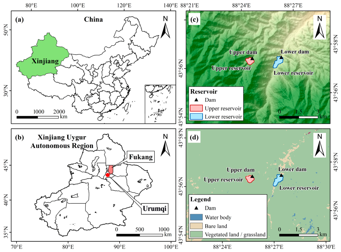
This study focuses on the Fukang Pumped Storage Hydropower (PSH) station, located in Fukang City, Changji Hui Autonomous Prefecture, Xinjiang Uygur Autonomous Region, China. Fukang has a permanent population of approximately 181,000 and is characterized by a typical temperate continental arid climate, with a mean annual air temperature of about 8.1 °C and a mean annual precipitation of about 134.8 mm [20]. As the first GW-level PSH facility in Xinjiang, the station has a total installed capacity of 1.2 gigawatt (GW) and consists of an upper and a lower reservoir. The upper reservoir uses the natural Tianshan Tianchi Lake, at an elevation of approximately 1910 m, whereas the lower reservoir is newly constructed on the piedmont alluvial–proluvial fan at an elevation of about 480 m. The study area is located at the northern foot of the eastern Tianshan Mountains beneath Bogda Peak (88.00° E–89.25° E, 41.75° N–44.00° N). Influenced jointly by the high-elevation mountain terrain to the south and the piedmont plain to the north, the area exhibits a pronounced mountain–piedmont climatic gradient: the upper reservoir in the Tianchi region is relatively cold and humid, whereas the lower reservoir in the piedmont zone is warmer and drier, with stronger evaporative demand. This environmental contrast provides the regional background for analyzing thermal-state responses and evaporation differences within the dual-reservoir system. In addition, the study area exhibits a heterogeneous land-cover background characterized by open water, bare land, and vegetated or grassland surfaces, which together shape the local environmental setting of the dual-reservoir system. Figure 1 shows the geographic location of the Fukang PSH station, the surrounding landform, the positions of the upper and lower reservoirs and their dams, and the land-cover background of the study area.

The Fukang PSH station is a suitable case for evaluating evaporation effects because it combines a high-elevation natural upper reservoir, a newly constructed lower reservoir on the piedmont plain, and a large elevation difference within an arid-region water-resource setting. This configuration creates contrasts in meteorological forcing, reservoir thermal inertia, and operational water-level response, allowing thermal, geometric, and exchange-flow controls on evaporation to be evaluated within one engineering system.

2.2. Data Sources and Preprocessing

To represent meteorological forcing in mountainous canyon terrain, this study used a dual-source forcing strategy. Hourly forcing series were constructed from ground-station observations and ERA5 reanalysis, and both datasets drove the same model structure and parameter set. Station forcing was used for the primary attribution analysis, while ERA5 forcing provided an independent benchmark for the direction and magnitude of the main responses. The simulation period extends from 1 January to 31 December 2024, and the model reconstructs evaporation, heat budgets, and scenario attribution using hourly meteorological and operational inputs.

Table 1. Main datasets used in this study and their basic information.

Product Name	Spatial Resolution	Temporal Resolution	Period Used	Data Link/DOI
ERA5 reanalysis data	~0.25° (~31 km)	Hourly	1 January 2024 to 31 December 2024	Copernicus Climate Change Service (C3S) https://cds.climate.copernicus.eu/ (accessed on 20 November 2025) [21]
Hourly observations from Tianchi Meteorological Station (Station ID: 51470)	Point observation	Hourly	1 January 2024 to 31 December 2024	China Meteorological Data Service Centre https://data.cma.cn/dataService/cdcindex/datacode/A.0012.0001/show_value/normal.html (accessed on 20 November 2025)
Hourly observations from Fukang Meteorological Station (Station ID: 51377)	Point observation	Hourly	1 January 2024 to 31 December 2024	China Meteorological Data Service Centre https://data.cma.cn/dataService/cdcindex/datacode/A.0012.0001/show_value/normal.html (accessed on 20 November 2025)

summarizes the main datasets used in the analysis. The processed forcing datasets and model-output figures are provided in the Supplementary Materials.

2.2.1. ERA5 Reanalysis Data

ERA5 is the fifth-generation global atmospheric reanalysis dataset released by the European Centre for Medium-Range Weather Forecasts (ECMWF) [21]. Although its local representation in mountainous terrain may still be affected by elevation-related bias [22], it remains suitable as a regional-scale background forcing dataset. It features hourly temporal resolution and a spatial resolution of approximately 31 km. For this study, hourly data covering the research area were obtained from the Copernicus Climate Change Service (C3S) platform. The symbols, units, and roles of the ERA5 variables used in the evaporation–energy calculations are summarized in

Table 2. ERA5 variables employed in this study and their physical roles.

Category	Full Variable Name	Code	Unit	Physical Significance and Model Application
Thermodynamic Parameters	2 m temperature	T2m	K	Air temperature: it determines the temperature gradient driving sensible heat flux and serves as the baseline for calculating saturated vapor pressure.
	2 m dewpoint temperature	Td2m	K	Dewpoint temperature: it represents the actual moisture content, used to derive relative humidity.
Dynamic Parameters	10 m u/v component of wind	u10/v10	m s−1	Wind vector: components are used to compute the 10 m scalar wind speed. This variable is denoted as Ws and is used consistently as the aerodynamic wind-speed input in the evaporation calculation.
	Surface pressure	sp	Pa	Surface pressure: it is used for calculating air density and the psychrometric constant and for correcting altitude effects.
Radiation Parameters	Surface net solar radiation	Rssr	J m−2	Net shortwave radiation: it is the primary energy source for water-body heating.
	Surface net thermal radiation	Rstr	J m−2	Net longwave radiation: it is the net result of the longwave radiation budget at the surface.

.

The raw ERA5 data were obtained in the NetCDF format, comprising multi-dimensional (longitude, latitude, time) grid data. The data-processing workflow involved the following key steps:

(1) Spatiotemporal Dimensionality Reduction and Alignment

Given the adoption of a lumped model in this study, the multi-dimensional gridded data required reduction to a single time series. Spatial Dimension: Grid data covering the upper and lower reservoir areas of the Fukang PSH station were extracted. Spatial averaging was performed across longitudinal and latitudinal dimensions to eliminate spatial heterogeneity at the grid scale. Temporal Dimension: The timestamps of the raw data were originally in Coordinated Universal Time (UTC). These were converted to Beijing Time (UTC + 8) by adding an 8 h offset, and the data were subsequently truncated to the full-year simulation period from 1 January to 31 December 2024.

(2) Conversion of Basic Meteorological Element

To align with the driving variables required by the model, raw physical quantities underwent unit standardization and vector synthesis. Air Temperature and Pressure: The 2 m air temperature (T_2m) was converted from Kelvin (K) to degrees Celsius (°C), and the surface pressure (P) was converted to the standard unit of kPa. Wind Speed (W_s): The raw data provided the 10 m zonal wind component (u₁₀) and meridional wind component (v₁₀). The 10 m scalar wind speed was calculated using the vector synthesis formula and then denoted as W_s for the aerodynamic term:

$$W_s=\sqrt{u_{10}^2+v_{10}^2}$$

(1)

(3) Calculation of Physical Quantities

Relative humidity (RH) and the associated thermodynamic variables (e_s, e_a, Δ, γ, etc.) were calculated using the standard formulations recommended by FAO-56 [23,24], with all units consistently harmonized (Equations (2)–(4)). Specifically, e_s was determined from air temperature, e_a was equivalently derived from dewpoint temperature, and RH was computed as e_a/e_s and constrained to the range [0, 100%]. This treatment was intended to maintain consistent variable definitions and dimensional systems between ERA5- and station-driven forcings [25].

$$e_s(T_{2m})=0.6108\exp \left({\displaystyle \frac{17.27T_{2m}}{T_{2m}+237.3}}\right)$$

(2)

$$e_a=e_s(T_{d2m})=0.6108\exp \left({\displaystyle \frac{17.27T_{d2m}}{T_{d2m}+237.3}}\right)$$

(3)

$$RH={\displaystyle \frac{e_a}{e_s(T_{2\mathrm{m}})}}\times 100\%$$

(4)

Surface Net Radiation (R_n): The surface net shortwave radiation (R_ssr) and surface net longwave radiation (R_str) provided by ERA5 are in units of hourly accumulated energy (J/m²). To convert these into the average radiative power (W/m²) required by the model, temporal averaging was performed. Unlike ground station data, which require the estimation of longwave radiation, ERA5 directly provides the net longwave component accounting for cloud and atmospheric counter-radiation effects. Therefore, the total net radiation is calculated as follows:

$$R_n={\displaystyle \frac{R_{ssr}+R_{str}}{3600}}$$

(5)

where 3600 represents the number of seconds in one hour. This step completes the physical dimensional conversion from “accumulated energy” to “instantaneous flux”.

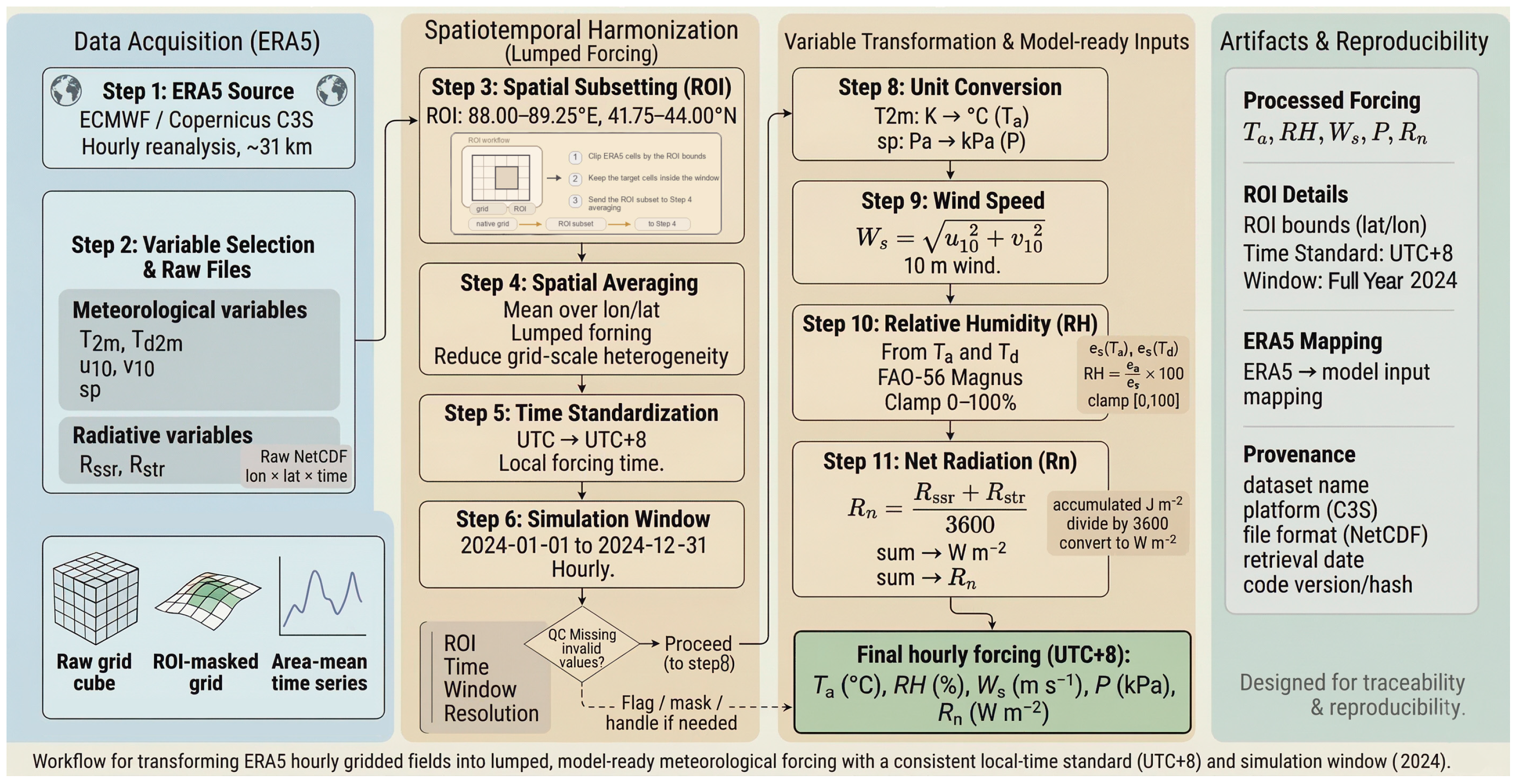
To improve the readability and traceability of the methodological workflow, Figure 2 summarizes the complete processing pipeline for ERA5 reanalysis data, from data acquisition and spatiotemporal alignment to variable transformation and construction of model inputs. This pipeline ensures consistency between ERA5- and station-driven forcings in time step, time zone, and variable dimensions, thereby supporting subsequent benchmark simulations and robustness checks.

2.2.2. In Situ Ground Meteorological Station Data

To precisely capture the local microclimate characteristics of the upper and lower reservoirs, hourly in situ data from two national meteorological stations were incorporated. Meteorological forcing data for the upper reservoir were sourced from the Tianchi Meteorological Station (Station ID: 51470; elevation: 1942 m), whereas data for the lower reservoir were obtained from the Fukang Meteorological Station (Station ID: 51377; elevation: 452 m). The two stations represent the main meteorological boundary characteristics of a high-mountain cold-humid environment and a piedmont arid environment, respectively.

(1) Time Series Construction and Alignment: Raw meteorological data were stored in a tabular format, containing timestamps (year, month, day, hour), atmospheric pressure (hPa), air temperature (°C), wind speed (m/s), relative humidity (%), and total solar radiation (MJ/m²). First, temporal information was extracted from the raw dataset to construct a continuous hourly time series. To maintain a consistent temporal resolution across variables and alignment with the full-year simulation period (1 January to 31 December 2024), linear interpolation was applied to resample all raw data to the model time step. During this process, duplicate timestamps were removed to avoid repeated records and keep a unique time series.

(2) Extraction of Meteorological Variables: Air temperature (T_a), relative humidity (RH), wind speed (W_s), atmospheric pressure (P), and total solar radiation (R_s) were extracted from the processed time series and utilized as the primary driving inputs for the model.

(3) Calculation of Radiation Components. Since the in situ data only provided hourly accumulated total solar radiation (MJ/m²) rather than the instantaneous power and net radiation values required for physical calculation, the following standardization steps were adopted:

Solar Radiation Power Conversion: First, the unit of total solar radiation (R_s) was converted from accumulated energy to average radiative power, R_sw (W/m²). According to the FAO-56 meteorological data-processing standard [23], the conversion formula is:

$$R_{\mathrm{SW}}=R_{\mathrm{S}}\times {\displaystyle \frac{{10}^6}{3600}}$$

(6)

where R_sw represents the hourly average solar radiation power (W/m²).

Net Shortwave Radiation (R_ns) Calculation: Considering the reflection of solar radiation by the water surface, net shortwave radiation was derived by subtracting the reflected radiation from the incident radiation [26]:

$$R_{\mathrm{ns}}=(1-\alpha )\times R_{sw}$$

(7)

where R_ns is the net shortwave radiation (W/m²), and alpha is the water-surface albedo. For deep reservoirs, an empirical value of alpha = 0.07 is adopted in this study [26].

Net Longwave Radiation (R_nl) Estimation: Because station observations did not directly include atmospheric longwave radiation, a Brunt-like dynamic empirical formula based on air temperature and humidity was used for estimation. This method effectively captures the longwave radiative cooling effects under nocturnal and varying humidity conditions [27]:

$$R_{\mathrm{nl}}=-\sigma {(T_a+273.15)}^4\cdot (a-b\sqrt{e_a})$$

(8)

where R_nl is the net longwave radiation (W/m²), sigma is the Stefan–Boltzmann constant (5.67 × 10⁻⁸ W·m⁻²·K⁻⁴), T_a is the air temperature, and e_a is the actual vapor pressure (kPa). Coefficients a and b are set to 0.34 and 0.14, respectively, following Brunt [27]. Compared with a fixed empirical value, this formulation better captures longwave radiative cooling under nighttime and varying humidity conditions.

Total Net Radiation (R_n,net) Calculation: The total net radiation required by the model was obtained as the sum of the net shortwave radiation and the estimated net longwave radiation [27]:

$$R_{\mathrm{n},\mathrm{net}}=R_{ns}+R_{nl}$$

(9)

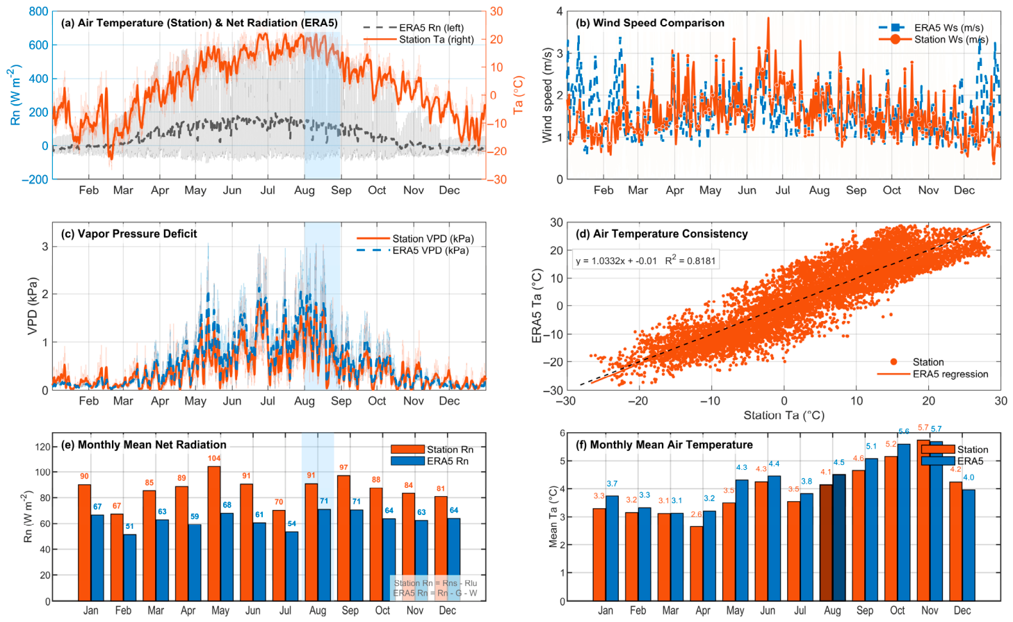
To evaluate how well ERA5 represents the meteorological forcing boundaries in this complex terrain, a combined time series and consistency assessment was conducted for the key evaporation drivers, including air temperature (T_a), net radiation (R_n), wind speed (W_s), and vapor pressure deficit (VPD) (Figure 3). Panels (a–c) show the temporal evolution of the main drivers, whereas panels (d–f) evaluate the consistency of air temperature, VPD, and net radiation using variable-specific comparison plots, the identity line (y = x), fitted regression lines, and the statistical metrics R², concordance correlation coefficient (CCC), RMSE, and bias. R² describes explained variance, CCC measures agreement with the 1:1 line, RMSE gives the absolute error scale, and bias denotes ERA5 minus station observations.

Based on Figure 3, two independent hourly meteorological forcing datasets were constructed from ERA5 and station observations and were used to drive the model under the same structure and parameter set. The main attribution analysis is based on station forcing, whereas the ERA5-driven results are retained as an independent benchmark to test the directional and magnitude robustness of the main conclusions. Differences between the two forcings are not used for reverse calibration; instead, they are used to characterize the smoothing effect of reanalysis data and differences in the radiation-estimation chain under complex terrain, thereby improving the transferability of the conclusions.

The station–ERA5 consistency statistics are summarized in

Table 3. Consistency metrics between ERA5 and station meteorological forcing.

Reference	Variable	R2	CCC	RMSE	Bias
Upper station	Air temperature	0.946	0.964	3.31	0.10
Upper station	Wind speed	0.011	0.069	1.84	−1.05
Upper station	Net radiation	0.914	0.924	78.39	−23.68
Upper station	Vapor pressure deficit	0.869	0.909	0.23	0.09
Lower station	Air temperature	0.952	0.900	6.98	−4.72
Lower station	Wind speed	0.072	0.262	1.23	0.05
Lower station	Net radiation	0.913	0.934	71.16	−16.73
Lower station	Vapor pressure deficit	0.900	0.647	0.87	−0.48

. Air temperature and net radiation show high agreement at both stations, whereas wind speed shows weaker point-scale consistency. Therefore, station observations are used as the primary forcing for attribution, and ERA5 is retained as an independent benchmark for directional robustness.

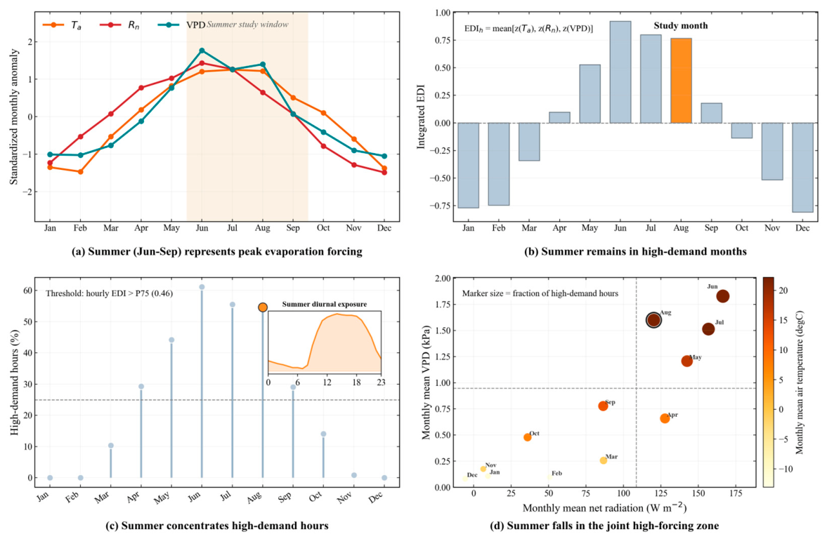
After the consistency assessment of the meteorological forcing, an annual meteorological background figure based on station forcing was further introduced (Figure 4). Figure 4 describes the position of summer (June–September) within the annual evaporative-forcing regime from four perspectives: standardized monthly anomalies, the composite evaporative-demand index (EDI), the fraction of high-demand hours, and the joint distribution of net radiation and VPD. The hourly EDI is calculated from standardized hourly air temperature, net radiation, and vapor pressure deficit as follows. where z(·) denotes standardization over the full-year hourly series. High-demand hours are identified when EDI_h exceeds the 75th percentile of the annual distribution. This figure provides the annual meteorological boundary and summer high-evaporation background for the annual attribution and dispatch–meteorology coupling analyses.

$$ED{I}_h={\displaystyle \frac{1}{3}}\left[z(T_{a,h})+z(R_{n,h})+z(VP{D}_h)\right]$$

(10)

2.3. Hydrodynamic–Thermal Coupled Model

To represent the coupled variations in water level, surface area, and thermal state induced by high-frequency PSH operation, a one-dimensional lumped thermo-hydrodynamic model was developed for evaporation-response calculation and scenario-based attribution under unified meteorological forcing and operating conditions.

2.3.1. Model Framework

The model comprises two interconnected modules: the hydrodynamic module and the thermal module. The hydrodynamic module calculates the water-mass balance of the upper and lower reservoirs based on station scheduling rules (pumping/generation flow rates), thereby deriving the time-varying water levels and surface areas. The thermal module computes the evolution of water temperature and surface evaporation flux based on meteorological forcing data and the water body energy balance equation. These two modules achieve bidirectional coupling through two key variables: water temperature and water surface area. Water temperature determines the evaporation rate, while the surface area determines the total evaporation volume. Conversely, evaporation induces water loss and heat dissipation, creating a feedback loop that influences water levels and temperatures.

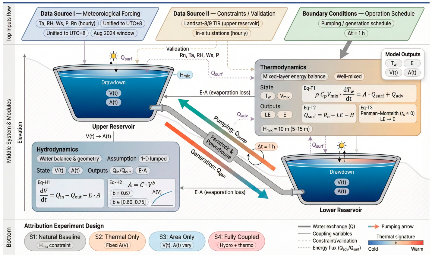
In this study, the coupled water-mass and energy conservation equations were solved using a unified time step (Δt = 1 h). The water-mass balance was used to update reservoir storage V, and the surface area A was obtained from the area–storage relationship A (V). The energy balance was used to update the mixed-layer water temperature T_w. The net surface heat flux comprised net radiation R_n, latent heat flux LE, and sensible heat flux H, and LE was computed using the Penman [15] open-water combination equation (expressed in Penman–Monteith notation with r_s ≈ 0). Here, A serves as the geometric scale for integrating evaporative volume loss, whereas T_w serves as the state variable controlling the thermal driving of evaporation. Together, they determine evaporative volume loss and its feedback on the water and energy budgets. Thermal coupling between the upper and lower reservoirs was achieved through exchange flows that transport enthalpy. This process was represented by an advective heat term, Q_adv, which couples the temperature evolution of the two reservoirs through the energy equations.

Based on the above structure, the model is used for evaporation-response calculation, scenario comparison, and dominant-mechanism identification under unified meteorological forcing and operation-induced disturbance. For natural stratification in the upper reservoir, an effective mixed-layer-depth parameterization is adopted in S₁. Under strong exchange conditions (S₂ and S₄), a dynamically fully mixed approximation is used to represent the thermal response under operational disturbance [28]. The overall coupling framework is summarized in Figure 5.

2.3.2. Hydrodynamic Process Model

The model treats the upper and lower reservoirs as two interconnected water bodies. For either reservoir, the change in water volume follows the ordinary differential equation given below [29]:

$${\displaystyle \frac{dV}{dt}}=Q_{\mathrm{in}}-Q_{\mathrm{out}}-Q_{evap}$$

(11)

where V is the reservoir storage volume (m³); t is time (s); Q_in and Q_out are the inflow and outflow rates (m³/s), respectively, determined by the station operation schedule and the common scenario boundary; and Q_evap is the volumetric evaporation rate (m³/s), calculated by the thermal module. Direct precipitation is treated as a common atmospheric boundary across the compared scenarios and is not decomposed as an operational exchange term, so the factorial attribution isolates PSH-induced exchange, area, and thermal effects.

Surface area, A, is the critical geometric parameter determining total evaporation. The storage-area response is constrained by the reservoir operating boundary, with dead and normal storage of about 40.0 × 10⁴ and 705.0 × 10⁴ m³ for the upper reservoir and 111.0 × 10⁴ and 777.0 × 10⁴ m³ for the lower reservoir, respectively. Considering the topographical features of canyon-type and basin-type reservoirs in arid and semi-arid regions, the traditional linear area–volume assumption can lead to substantial errors. Assuming that the reservoir basin approximates an inverted conical geometry, the surface area and storage volume follow a power-law relationship. Related bathymetric volume–area–height and water-level–storage studies provide a basis for representing this geometric response [30,31]:

$$A\left(\mathrm{t}\right)=A_{max}\times {\left({\displaystyle \frac{V(t)}{V_{max}}}\right)}^b$$

(12)

where b is the basin-shape exponent that characterizes how sensitively surface area responds to storage variation. In this study, the area–volume power-law relationship is used to represent the A–V geometric response of the reservoir basin. For canyon-type basins, the A–V exponent is approximately 2/3 under an idealized inverted-cone representation; accordingly, b = 0.67 is adopted here as the central representative value. This choice is also consistent with the deep and narrow mountain-lake morphology of the upper reservoir (Tianchi), whose geometric scale is broadly comparable to the response of canyon-type lake–reservoir systems [32]. Furthermore, to cover possible basin-geometry differences within the study area, a structural uncertainty analysis is conducted over the range b = 0.60–0.75 to test the robustness of the main conclusions to geometric-parameter variation. Therefore, b is used here to represent the dominant geometric response of the canyon-type basin in the study area.

2.3.3. Thermal Process and Hydrodynamic Coupling

Water-temperature evolution follows the law of energy conservation. For pumped-storage reservoirs with substantial inflow and outflow exchange, the participating water body is represented in a lumped manner at the reservoir-operation attribution scale, and its transient heat balance is described as follows [33]:

$$\rho C_{p}V{\displaystyle \frac{d{T}_{\mathrm{w}}}{dt}}=Q_{surf}A+Q_{adv}$$

(13)

where ρ is the water density (1000 kg/m³); C_p is the specific heat capacity of water (4186 J/(kg·K)); and T_w is the mixed-layer water temperature (°C). The heat-storage term represents the “active water volume” that effectively participates in energy exchange. In S₁, heat storage was characterized by the surface mixed-layer volume A·H_mix. Under strong exchange disturbances (S₂/S₄), a dynamically fully mixed approximation was adopted, such that the full storage volume V participated in the energy-budget update, thereby capturing changes in thermal inertia induced by enhanced mixing.

Q_adv represents the advective heat flux induced by inflow and outflow. It is a key energy term distinguishing PSH systems from static lakes and characterizes the enthalpy transport associated with water exchange, calculated as follows [18,28]:

$$Q_{\mathrm{adv}}=\rho C_p{Q}_{\mathrm{in}}(T_{\mathrm{in}}-T_w)$$

(14)

where T_in is the inflow water temperature. For the upper reservoir, T_in is taken as the outflow temperature of the lower reservoir at the current time step, and vice versa. The conveyance-lag scale is shorter than the hourly model step: using a 1650 m conveyance length and a 6.5 m tunnel diameter gives estimated travel times of about 12.7 min for a single-unit flow of 71.6 m³/s and 6.4 min for a one-tunnel-two-unit flow of 143.2 m³/s. The same-time-step coupling therefore represents the hourly scale enthalpy exchange used in the attribution model. Q_surf is the net heat flux per unit water surface area (W/m²), determined by heat exchange at the air–water interface [28]:

$$Q_{\mathrm{surf}}=R_{\mathrm{net}}-LE-H$$

(15)

where R_net is the net radiation flux; LE is the latent heat flux; and H is the sensible heat flux.

2.3.4. Open-Water Penman Combination Equation

Evaporation in this study is calculated using the Penman [15] open-water combination equation. For consistency with the general Penman–Monteith variable system, the formulation is expressed in Penman–Monteith notation while setting the open-water surface resistance to r_s ≈ 0. The equation therefore contains both an energy-balance term and an aerodynamic term [14].

The latent heat flux LE (W/m²) is calculated as follows:

$$LE={\displaystyle \frac{\Delta (R_{\mathrm{net}}-G)+{\rho }_a{C}_p\frac{(e_s-e_a)}{r_a}}{\Delta +\gamma }}$$

(16)

For open water, the surface resistance is approximately r_s ≈ 0 because stomatal resistance is absent, and the aerodynamic term is expressed using a wind function (or, equivalently, an aerodynamic resistance rₐ). Therefore, the equation used here can be regarded as the open-water simplification of the Penman combination equation within the Penman–Monteith notation framework [15,34]:

In the above equation, Δ is the slope of the saturation vapor-pressure curve (kPa/°C), γ is the psychrometric constant, e_s is the saturation vapor pressure (kPa) calculated from water-surface temperature T_w, and e_a is the actual vapor pressure (kPa) calculated from air temperature T_a and relative humidity RH.

The wind function f(u) is critical to determining the accuracy of latent heat flux calculations. This study adopts the original Penman [15] wind function form, which has been verified in similar high-altitude arid basins [32]. Given that the model operates on an hourly time step and the energy balance equation is based on instantaneous power (W/m²), the original daily-scale empirical coefficients must undergo dimensional conversion. The coefficients were obtained by converting the original Penman [15] wind function from an “evaporation-rate form” to a “latent-heat-flux form”. Specifically, the aerodynamic term expressed as an evaporation depth (e.g., mm·d⁻¹) was multiplied by ρ_w λ/86,400 to yield W·m⁻², and the vapor-pressure deficit was consistently expressed in kPa. In addition, given the model time step (Δt = 1 h), both the radiative and aerodynamic terms were maintained in the same instantaneous flux units so that they could be directly summed. The modified energy-form wind function is:

$$f(u)\approx 74.42(1+0.536u_2)$$

(17)

where W_s is the wind-speed variable used in the aerodynamic term (m/s). ERA5 wind forcing is obtained from the 10 m u/v components, whereas station forcing uses the recorded near-surface wind speed; both are processed as hourly W_s and then passed through the same Penman wind-function form. The coefficient 74.42 has dimensions of W m⁻² kPa⁻¹. This treatment keeps the aerodynamic and radiative terms dimensionally consistent for the hourly evaporation calculations and scenario-based attribution analysis.

A wind-height diagnostic was further conducted following the FAO-56 logarithmic conversion, u₂ = u_z × 4.87/ln(67.8 z − 5.42), with z = 10 m for ERA5 wind components. For the 2024 ERA5 series, this conversion factor is 0.748; the annual mean wind speed changes from 1.60 m s⁻¹ at 10 m to 1.20 m s⁻¹ as a 2 m equivalent, and the corresponding Penman wind-function ratio is 0.893. Because the attribution analysis is primarily based on station forcing and ERA5 is used as an independent background benchmark, the manuscript reports a common W_s variable while interpreting it consistently with the forcing source.

Sensible heat flux H (W/m²) is estimated from the Bowen ratio, which helps enforce energy-budget closure [35]:

$$H=\beta \cdot LE=\gamma \cdot {\displaystyle \frac{T_w-T_a}{es-ea}}\cdot LE$$

(18)

Finally, the evaporation rate E_rate (m/s) can be directly derived from the latent heat flux:

$$E_{\mathrm{rate}} = {\displaystyle \frac{LE}{\rho w \cdot \lambda }}$$

(19)

where ρ_w is the water density (kg/m³), and λ is the latent heat of vaporization (J/kg).

By solving the above system of equations simultaneously, the model provides hourly responses of water level, water temperature, and evaporation under unified meteorological forcing and operating conditions, thereby supporting subsequent scenario comparison and quantitative attribution analysis. The evaporation flux enters the water-balance equation as a loss term and the energy-balance equation as a latent-heat dissipation term, therefore acting as a key coupling term between hydrodynamic and thermal processes.

2.3.5. Coupling Mechanism and Numerical Solution

The water-balance and energy-balance equations were integrated synchronously using a fixed time step of Δt = 1 h. At each time step, the exchange flow Q(k) was prescribed by the operation schedule. Reservoir storage was then updated to V(k + 1), and the surface area A(k + 1) was obtained from A(V). Net radiation and aerodynamic terms were computed using A(k + 1) and the meteorological forcing to obtain the latent heat flux LE(k + 1) and evaporative volume loss E(k + 1). The evaporative loss was then substituted back into the water-balance equation to achieve water-budget closure at the model time step. In the energy equation, the mixed-layer temperature T_w(k + 1) was updated using Q_adv and Q_surf, with LE and H included as dissipation terms to maintain energy consistency [18,36]. At the monthly accumulation scale, numerical consistency was further evaluated using the system-scale energy-closure residual (see Section 3.3).

Water-storage boundary behavior and mass-balance residuals were diagnosed under the same model structure. The baseline diagnostics in

Table 4. Baseline water-storage boundary and mass-balance diagnostics. Storage is in 10⁶ m³, area is in 10⁴ m², and residual is in m³.

Scenario	Reservoir	Mean Storage	Storage Range	Mean Area	Boundary h	Residual
S1	Upper reservoir	7.45	7.11–7.80	50.44	19	9.43 × 10−9
S4	Upper reservoir	4.11	1.03–6.74	33.18	0	2.71 × 10−8
S1	Lower reservoir	5.58	5.24–5.90	47.35	0	−1.42 × 10−8
S4	Lower reservoir	5.90	3.19–9.00	48.70	0	2.71 × 10−8

show that storage and area remain within the prescribed model boundaries and that water-balance residuals are close to numerical zero, supporting the use of the scenario outputs for evaporation attribution.

2.4. Four-Scenario Orthogonal Attribution Experiment Design

The scenario analysis covers one complete operating and meteorological year (1 January–31 December 2024). The year provides continuous hourly station and ERA5 forcing, includes both cold and warm seasons and the high-evaporation period, and allows the same dispatch rules to be applied throughout a full annual cycle. This annual window therefore supports full-year process attribution under consistent meteorological and operational boundaries, and the same framework can be applied to additional hydrological years and dispatch regimes for inter-annual comparison [37].

The scenario definitions and dispatch windows used in the attribution and sensitivity analyses are summarized in

Table 5. Operational scenarios and dispatch parameters used in the attribution and sensitivity analyses.

Scenario	Qin/Qout (m3 s−1)	Pump Hours	Generation Hours	Cycles	Operating h d−1	Treatment
S1 natural baseline	0/0	none	none	0	0	no exchange; upper S1 Hmix = 10 m
S2 thermal-only	180/180	baseline schedule	baseline schedule	2	16	thermal exchange retained; area fixed at initial value
S3 area-only	180/180	baseline schedule	baseline schedule	2	16	dynamic area retained; water temperature inherited from S1
S4 fully coupled	180/180	baseline schedule	baseline schedule	2	16	dynamic storage, area, water temperature, and advective heat
Low dispatch	180/180	00:00–05:00	18:00–22:00	1	11	dispatch sensitivity regime
Baseline dispatch	180/180	00:00–07:00	11:00–14:00; 19:00–22:00	2	16	main dispatch regime
Enhanced dispatch	180/180	00:00–06:00; 12:00–14:00	08:00–10:00; 17:00–23:00	2	20	dispatch sensitivity regime

.

S₁ natural baseline: This scenario represents the attribution baseline without PSH exchange flow. Initial storage and surface area are prescribed from the same reservoir geometry used in the other scenarios, evaporation-driven storage change is allowed at the hourly step, and natural external boundaries are kept identical across scenarios so that the scenario differences isolate operational area and thermal effects. The upper reservoir (Tianchi) is a deep alpine lake with pronounced summer thermal stratification, where solar heating is primarily concentrated above the thermocline. Accordingly, an effective mixed-layer-depth constraint is introduced in S₁, and the energy balance is applied to the active near-surface layer. Previous studies indicate that the summer thermocline in Lake Tianchi is mainly distributed within approximately 2–18 m [38]. On this basis, H_mix = 10 m is adopted as the central setting, and sensitivity tests are conducted over 5–15 m to cover possible variations in effective mixed-layer depth under relatively strong to relatively weak stratification [19].

$$\Delta E_i=E(S_4)-E(S_2)-E(S_3)+E(S_1)$$

(20)

Therefore, the following decomposition holds:

$$\Delta E= \Delta Et+ \Delta Ea+ \Delta Ei$$

(21)

In the above equation, the sign and magnitude of ΔE_i quantify the degree of nonlinear synergy or antagonism between the area and thermal effects under fully coupled conditions, thereby providing a consistent quantitative definition for interpreting main and interaction effects in Section 3.

3. Results and Analysis

3.1. Variation Characteristics of Total System Evaporation

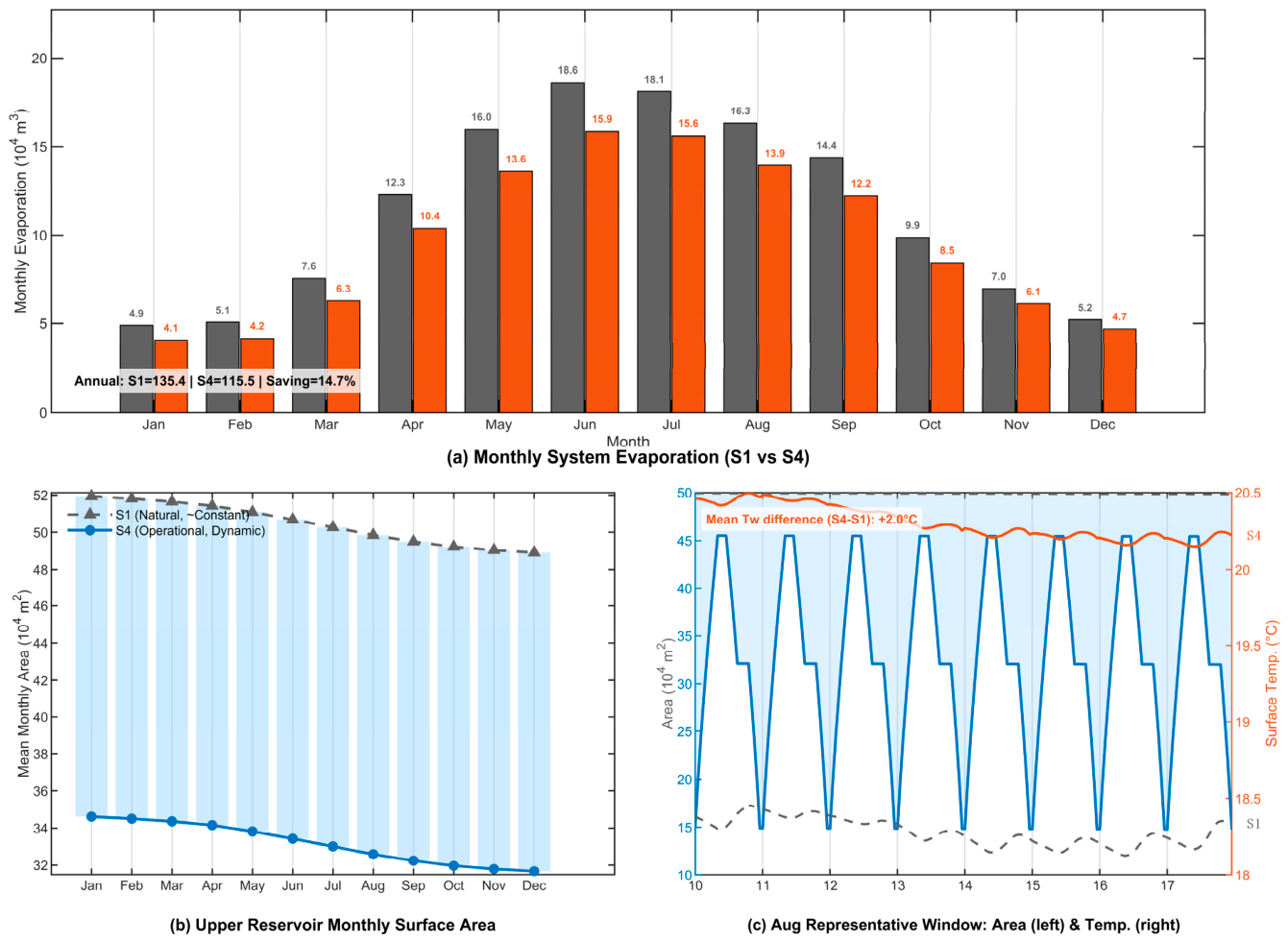
The annual simulation results (Figure 6a) indicate that, for the full year of 2024, the fully coupled operational scenario (S₄) produces a lower system-scale evaporation volume than the natural baseline (S₁). Here, system-scale evaporation denotes the sum of open-water evaporation from the upper and lower reservoirs and does not include non-open-water hydraulic structures such as conveyance tunnels or pressure pipelines. On the annual scale, system evaporation decreases from 135.36 × 10⁴ m³ under S₁ to 115.45 × 10⁴ m³ under S₄, corresponding to a net reduction of 19.91 × 10⁴ m³ or 14.7%. Evaporation reduction denotes the modeled difference in evaporation volume between scenarios.

In terms of intra-annual distribution, the difference between S₁ and S₄ is concentrated mainly from late spring to autumn, when evaporative demand is relatively high, whereas winter evaporation is smaller in absolute magnitude but remains part of the full-year hourly calculation. Under the baseline schedule, the low-temperature-season diagnosis gives S₁ = 15.16 × 10⁴ m³ and S₄ = 12.90 × 10⁴ m³, with a winter net reduction of 2.27 × 10⁴ m³, accounting for about 11.4% of the annual system net reduction. Figure 6b shows that, under S₄, the upper-reservoir surface area contracts and expands with operational scheduling, and its time-mean surface area is lower than that under the full-water natural baseline (S₁). This reduces evaporative accumulation at the volumetric scale. Figure 6c presents an August high-evaporation-period example to illustrate the coupled area–temperature process; the evaporation totals and attribution results are calculated for the full year of 2024.

A net evaporation reduction at the annual system scale does not imply consistent responses of the upper and lower reservoirs to operational disturbances. The two reservoirs differ in elevation, local meteorological conditions, water-temperature background, and the direction of exchange-flow enthalpy transport. As a result, the thermal main effect, area main effect, and interaction term differ in sign and magnitude between the two reservoirs. Therefore, annual evaporation changes in the upper and lower reservoirs are attributed separately using the four-scenario factorial decomposition, and the mechanistic differences are interpreted (Figure 7).

3.2. Physical Mechanism Attribution: Heterogeneous Responses of Upper and Lower Reservoirs

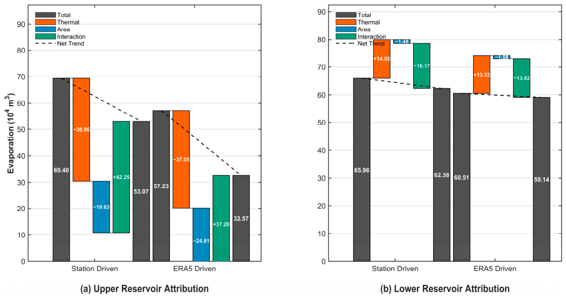
Changes in system-wide total evaporation arise from the differentiated responses of the upper and lower reservoirs to the combined thermal disturbances and geometric changes. Figure 7 presents the attribution results from the four-scenario factorial experiment, which decomposes the operation-induced evaporation change relative to the natural baseline into thermal and area main effects and an interaction term, thereby enabling interpretation of the mechanistic differences between the two reservoirs.

3.2.1. Upper Reservoir: Main-Effect Evaporation Reduction and Positive Interaction Offset

As shown in Figure 7a, the upper reservoir exhibits a response characterized by main-effect evaporation reduction and positive interaction offset under annual operational disturbance. On the annual scale, fully coupled operation reduces upper-reservoir evaporation from 69.40 × 10⁴ m³ to 53.07 × 10⁴ m³, corresponding to a net reduction of 16.33 × 10⁴ m³. Mechanistically, the thermal-only scenario (S₂) reduces evaporation by 38.96 × 10⁴ m³ relative to the natural baseline, and the area-only scenario (S₃) reduces evaporation by 19.63 × 10⁴ m³. This indicates that both the annual thermal trajectory and surface-area contraction can reduce upper-reservoir evaporation. However, the interaction term is +42.26 × 10⁴ m³, offsetting much of the reduction implied by the linear sum of the two main effects. Thus, the annual result does not support interpreting the thermal disturbance in the upper reservoir simply as an evaporation-enhancing effect. Instead, it should be understood as a non-additive response shaped jointly by water-body thermal inertia, operational mixing, heat storage, and surface-area contraction.

3.2.2. Lower Reservoir: Competition Between Thermal Enhancement and Negative Interaction Reduction

As shown in Figure 7b, annual evaporation in the lower reservoir decreases from 65.96 × 10⁴ m³ to 62.38 × 10⁴ m³, corresponding to a net reduction of 3.58 × 10⁴ m³. Unlike the upper reservoir, the thermal-only scenario increases evaporation by 14.05 × 10⁴ m³ relative to the natural baseline, indicating that exchange-flow-induced thermal-state changes can enhance evaporation per unit area in the lower reservoir. The area term is −1.46 × 10⁴ m³ and therefore contributes only weakly to evaporation reduction, whereas the interaction term is −16.17 × 10⁴ m³ and forms the main source of the net reduction. This result shows that the lower-reservoir response is not simply the result of area contraction, but a net effect produced when thermal enhancement is offset by negative area–thermal coupling. The two reservoirs therefore follow different attribution pathways: the upper reservoir is dominated by main-effect reductions with positive interaction offset, whereas the lower reservoir is governed by competition between thermal enhancement and negative interaction reduction.

3.3. Energy-Budget Analysis: Further Physical Interpretation

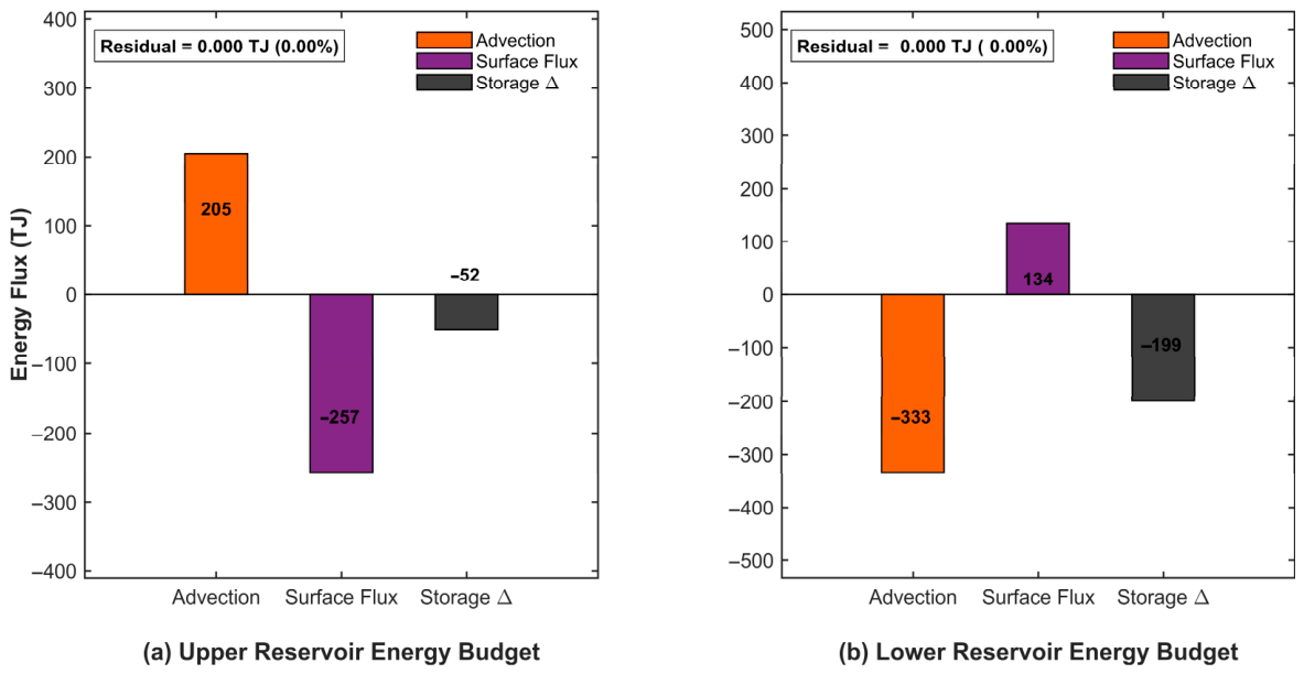
To reveal the physical basis of how station operation alters water temperature and evaporation, this study further interprets the annual results from the perspective of the energy budget. Figure 8 quantifies annual cumulative advective heat transport, net air–water surface heat flux, and heat-storage change for the upper and lower reservoirs.

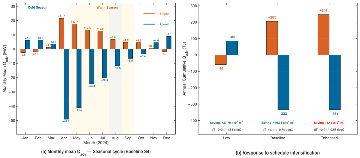
The energy-budget results in Figure 8 indicate that advective heat transport (Q_adv) plays a dominant role in redistributing heat between the two reservoirs, but its annual cumulative magnitude does not simply cancel between reservoirs. The upper reservoir receives +205 TJ of advective heat input, while its net air–water surface heat flux is −257 TJ and heat-storage change is −52 TJ, with a closure residual of 9.24 × 10⁻¹⁴ TJ (3.60 × 10⁻¹⁴%). The lower reservoir loses −333 TJ through advective heat transport, while its net surface heat flux is +134 TJ and heat-storage change is −199 TJ, with a closure residual of −1.99 × 10⁻¹³ TJ (−5.97 × 10⁻¹⁴%). The opposite signs of the advective terms confirm exchange flow as a key pathway of inter-reservoir heat redistribution. However, because of differences in reservoir storage, water temperature, operation timing, and surface fluxes, the annual cumulative advective heat terms should be interpreted as reservoir-specific energy-budget components rather than as simple system-level cancelation.

The corresponding numerical closure diagnostics are given in

Table 6. Energy-closure diagnostics under the baseline dispatch regime. All energy terms are in TJ.

Volume	Qadv	QsurfA	dS	Residual	Residual %
Upper reservoir	205.04	−256.57	−51.52	9.24 × 10−14	3.60 × 10−14
Lower reservoir	−333.25	134.44	−198.81	−1.99 × 10−13	−5.97 × 10−14
Two-reservoir system	−128.21	−122.12	−250.33	−1.07 × 10−13	5.97 × 10−14

. Under the baseline dispatch, closure residuals remain close to numerical zero at reservoir and system scales, indicating that the heat-budget decomposition is internally consistent under the adopted sign convention.

From the intra-annual perspective, advective heat transport does not act merely as an internal term in the cumulative energy decomposition, but continuously modifies the thermal states of the two reservoirs across months (Figure 9). Under the baseline schedule, Q_adv is positive in the upper reservoir for most months, corresponding to heat input from exchange flow, whereas Q_adv is negative in the lower reservoir for most months, corresponding to heat export. The annual result emphasizes seasonal heat redistribution: advective heat transport is stronger from spring to summer and weaker in winter, but its annual accumulation still constrains heat storage and evaporation attribution in both reservoirs.

3.4. Sensitivity and Meteorological Driver Analysis

3.4.1. Robustness Analysis of Model Structural Parameters

(1) Sensitivity to the effective mixed-layer depth (H_mix): In the natural baseline scenario (S₁), the effective mixed-layer depth is an important thermal boundary affecting the upper-reservoir thermal state and evaporation response. Based on observations showing that the summer thermocline in Tianchi is mainly distributed within approximately 2–18 m [38], H_mix = 10 m is adopted as the central setting, and model responses are tested over the range of 5–15 m to cover possible variations in effective mixed-layer depth from relatively strong to relatively weak stratification. The results (

Table 7. Sensitivity of upper-reservoir evaporation response to H_mix.

Scenario	Hmix (m)	Physical Meaning	S1: (104 m3)	S4: (104 m3)	Evaporation Reduction Rate	Variation vs. Baseline
Shallow	5.0	Strong stratification/high stability	8.68	7.26	16.36%	−1.36%
Baseline	10.0	Typical thermocline depth	8.80	7.26	17.50%	0.00%
Deep	15.0	Weak stratification/enhanced mixing	8.85	7.26	17.97%	+0.57%

) show that increasing mixed-layer depth increases thermal inertia in S₁, whereas the upper-reservoir evaporation response remains generally stable. When H_mix varies within this range, natural evaporation in the upper reservoir changes by only −1.28% to +0.64%; across all tested depths, the relative evaporation reduction in the upper reservoir remains positive, ranging from 16.36% to 17.97%. This indicates that, within the tested mixed-layer-depth range, the direction of relative evaporation reduction in the upper reservoir is insensitive to H_mix perturbation, and structural-parameter variation does not alter the basic role of area change in evaporation attribution.

(2) Basin-geometry sensitivity represented by the reservoir exponent (b): The basin-shape exponent b characterizes how sensitively surface area responds to storage drawdown in the area–storage power-law relationship. In this study, b is treated as an equivalent geometric-response parameter constrained by the reservoir level-storage boundary and tested over b = 0.60–0.75 to bracket the response from a steeper to a gentler area–storage curve. The results (

Table 8. Sensitivity of upper-reservoir evaporation response to basin-shape exponent b.

Geometry Assumption	Shape Index B	S4: Operational Evaporation (104 m3)	Upper-Reservoir Relative Evaporation Reduction (S1 vs. S4)	Response Characteristic
Steep V-shape	0.60	6.92	21.42%	Positive evaporation reduction
Baseline	0.67	7.26	17.50%	Baseline response
Flat U-shape	0.75	6.65	24.38%	Positive evaporation reduction

) indicate that variations in b primarily affect the magnitude of surface-area contraction associated with drawdown under operation (S₄), thereby modulating the time-mean area response and the magnitude of the area term. Under the gentler-geometry assumption (b = 0.75), the relative evaporation reduction is 24.38%, and it remains 21.42% under the steeper assumption (b = 0.60). Together with the H_mix sensitivity results, the b-sensitivity test shows that the upper-reservoir relative evaporation reduction remains positive across the tested basin-geometry range and that the role of area change in evaporation attribution remains stable.

3.4.2. Dispatch-Regime Sensitivity and Meteorological Robustness

To examine how annual evaporation response varies with operating conditions and meteorological backgrounds, multiple dynamical scenarios were designed for sensitivity analysis. Here, dispatch regime is characterized by three quantifiable factors, i.e., the number of daily cycles n (pumping/generation frequency), the duration per cycle T (or the equivalent total daily operating time T_op), and the exchange-flow magnitude Q_max, which controls the amplitude of water-level and surface-area fluctuations. In Figure 10a, scenarios are grouped by n and T_op (low-frequency/baseline/enhanced) to test the nonlinear response of system-scale net evaporation reduction to dispatch regime. The results show that system-scale net evaporation reduction, defined as the total evaporation difference between the natural baseline (S₁) and fully coupled operation (S₄), does not vary monotonically with dispatch regime, but instead depends on the phase alignment or misalignment between water level–area variation and periods of high evaporative demand (high net radiation and VPD).

A winter contribution diagnosis was also conducted to identify the seasonal composition of the annual evaporation difference. Under the baseline schedule, the system-scale winter reduction is 2.27 × 10⁴ m³, accounting for 11.4% of the annual system reduction (

Table 9. Winter contribution to annual evaporation reduction under the baseline dispatch regime. Evaporation volumes are in 10⁴ m³.

Volume	S1 Winter	S4 Winter	Winter Reduction	Annual Reduction	Winter Share
Upper reservoir	8.38	5.84	2.53	16.33	15.5
Lower reservoir	6.79	7.05	−0.26	3.58	−7.3
Two-reservoir system	15.16	12.90	2.27	19.91	11.4

). This indicates that low-temperature months are included in the annual mass-balance diagnosis, while the dominant evaporation-response signal remains controlled by higher-demand operating periods.

Three representative dispatch regimes were used in the sensitivity analysis. The low-frequency regime represents one daily cycle for the evening peak (11 h d⁻¹). The baseline regime follows the S₄ two-cycle schedule with morning and evening peaks (16 h d⁻¹). The enhanced regime adds a midday pumping window for photovoltaic absorption (12:00–14:00) to the baseline schedule, increasing daily operation to 20 h d⁻¹.

The results indicate that changes in dispatch regimes exert a pronounced nonlinear influence on the system-scale evaporation-reduction effect. Figure 9b shows that system-scale net evaporation reduction is 37.70 × 10⁴ m³, 19.91 × 10⁴ m³, and −3.41 × 10⁴ m³ under the low, baseline, and enhanced scheduling regimes, respectively. The lower-intensity schedule corresponds to a larger annual net evaporation reduction, whereas the enhanced schedule does not expand the evaporation-reduction effect and instead shifts the system from evaporation reduction to evaporation increase. This occurs because the dispatch regime modifies not only exchange-flow heat transport, but also the phase relationship between water-surface exposure and periods of high evaporative demand. When the added pumping window overlaps with high net radiation and high VPD, the evaporation increment caused by surface-area expansion may exceed the benefit from thermal regulation, thereby weakening or reversing the net evaporation-reduction effect.

As also shown in Figure 9b, stronger advective heat transport and larger thermal-state anomalies do not necessarily translate into greater evaporation reduction. The evaporation response must therefore be evaluated jointly from exchange-flow heat transport, surface-area variation, and exposure during high-evaporation periods.

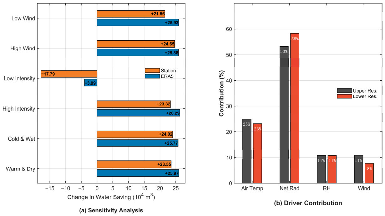
(2) Response under meteorological perturbation scenarios: To further test the stability of the conclusions under different meteorological boundaries, four disturbance scenarios were constructed: low wind, high wind, warm-dry, and cold-humid. The annual results show that different meteorological perturbations modify evaporation intensity and the magnitude of evaporation reduction, but do not remove the basic mechanism by which coupled area and thermal processes control the evaporation response. Relative to the baseline scenario, wind perturbations mainly affect the aerodynamic term, whereas warm-dry and cold-humid perturbations mainly modify evaporative demand through net radiation, VPD, and the air–water temperature difference. Figure 10a reports changes relative to the baseline scenario and is used to compare the relative sensitivity of system-scale net evaporation reduction under different meteorological perturbations.

(3) Contributions of meteorological factors: Figure 10b illustrates the relative driving weights of individual meteorological factors. On the annual scale, net radiation remains the dominant energy source, contributing approximately 53% and 58% for the upper and lower reservoirs, respectively. Air temperature contributes approximately 25% and 23%, reflecting the modulation of evaporative demand by seasonal temperature variation. Relative humidity contributes approximately 11%, and wind speed contributes approximately 11% and 8% for the upper and lower reservoirs, respectively. These results indicate that wind remains a non-negligible evaporation driver in arid, windy regions such as Xinjiang, but net radiation and air temperature together form the dominant annual thermal boundary.

4. Discussion

This study developed a hydrodynamic–thermal coupled model for high-frequency PSH operation in an arid region and used it to separate the main physical drivers of evaporative water consumption. In contrast to natural lakes or static reservoirs, PSH systems involve concurrent changes in surface area, exchange-flow heat transport, and reservoir thermal state. The following sections discuss how these coupled processes explain the simulated annual evaporation response, the associated energy-budget restructuring, and the sensitivity to dispatch and meteorological conditions.

4.1. Nonlinear Competition Between Area and Thermal Effects

Simulation results indicate that annual evaporation change is jointly controlled by surface-area variation, thermal-state restructuring, and their interaction, rather than by a single area or thermal mechanism. In the upper reservoir, both thermal-only and area-only effects reduce evaporation, but their combined response is substantially offset by a positive interaction term under fully coupled conditions. In the lower reservoir, the thermal-only effect enhances evaporation, the area effect is weakly negative, and the negative interaction term dominates the net evaporation reduction. This result shows that the key to understanding PSH evaporation response is not only whether operation reduces mean surface area, but also how operation timing reshapes water temperature, heat storage, and surface-area exposure during high-evaporation periods.

The interaction term shown in Figure 7 further indicates that the area and thermal effects are not independent under fully coupled conditions, but are linked through substantial nonlinear coupling. In the upper reservoir, both the thermal and area terms reduce evaporation on the annual scale, whereas the positive interaction term offsets part of the reduction implied by their linear sum. Its physical meaning is not a simple thermal enhancement of evaporation, but a non-additive response in which operational mixing, heat-storage change, and surface-area contraction jointly modify evaporation intensity per unit area and effective evaporating area. By contrast, in the lower reservoir, the thermal term enhances evaporation, the area term weakly reduces evaporation, and the negative interaction term dominates the net reduction. Thus, the two reservoirs follow distinct pathways within the same attribution framework: main-effect reduction with positive interaction offset in the upper reservoir and competition between thermal enhancement and negative interaction reduction in the lower reservoir.

4.2. Restructuring of Water Energy Budget by Operational Scheduling

Energy-budget analysis further reveals the fundamental thermodynamic characteristic that distinguishes PSH stations from natural water bodies: operation-induced advective heat transport not only alters the annual cumulative heat budget, but also continuously reshapes the thermal states of the upper and lower reservoirs at the seasonal scale. As shown in Figure 8, advective heat transport (Q_adv) is the most important internal heat-redistribution term between the two reservoirs. It appears as a net heat input to the upper reservoir and a net heat output from the lower reservoir, but the two annual cumulative terms do not simply cancel. The system-level energy interpretation should therefore consider advective heat transport, net air–water surface heat flux, and heat-storage change together, rather than relying only on the sign of the internal exchange term.

The scheduling-sensitivity results in Figure 9 further show that different scheduling regimes modify both advective heat-transport strength and surface-area exposure timing. Under the baseline scenario, the annual cumulative advective heat input is approximately +205 TJ for the upper reservoir and −333 TJ for the lower reservoir. The enhanced scenario further strengthens heat redistribution, but system-scale net evaporation reduction becomes −3.41 × 10⁴ m³. Therefore, advective heat transport is not merely an internal pathway in the energy budget; it is a dynamic constraint linking operation scheduling, reservoir thermal evolution, surface-area exposure, and evaporation response.

4.3. Temporal Effects of Dispatch–Meteorology Coupling

The sensitivity analysis reveals a key physical insight: evaporation reduction in pumped-storage hydropower does not increase monotonically with dispatch regime but instead depends on the phase relationship between hydrodynamically driven surface-area responses and the diurnal cycle of meteorological evaporative potential.

From the perspective of operation optimization, Figure 9 and Figure 10 jointly show that evaporation-reduction benefit depends on the timing of exposed surface area relative to evaporative demand, rather than on dispatch regime alone. The weaker schedule produces a larger annual net evaporation reduction, indicating that reduced surface-area exposure during high-evaporation periods can be more favorable than stronger exchange-flow thermal regulation. Although the enhanced schedule increases advective heat-transport intensity, the added pumping window overlaps with high radiation and high VPD, which can increase evaporative exposure and weaken the net reduction. Therefore, the evaporation effect of a dispatch scheme should be evaluated jointly from exchange-flow heat transport, surface-area amplitude, and exposure during high-evaporation periods.

This result has direct implications for comparing PSH operation schemes in arid regions. Under grid-regulation constraints, the phase relationship between water-level variation and the local diurnal cycle of evaporative demand is important. If high water level or larger surface area occurs mainly during nighttime or early-morning periods of low evaporative potential, while surface-area exposure is limited during midday periods of high radiation and high VPD, evaporative losses are more likely to be reduced. Conversely, simply increasing pumping-generating frequency or extending exchange-flow duration may yield a lower evaporation-reduction benefit when it increases exposure during high-demand periods.

4.4. Model Applicability and Future Perspectives

The existing sensitivity analyses and energy-closure results indicate that the conclusions regarding annual evaporation-change direction, heterogeneous upper- and lower-reservoir responses, and relative differences among scenarios are internally consistent. The energy-closure results further show that the system-scale evaporation response can be explained jointly by advective heat transport, air–water surface flux, and heat-storage change, providing a physical basis for reservoir-operation evaporation-response analysis, scenario comparison, and dominant-mechanism identification.

In terms of interpretation level, the present framework is suited to relative-change analysis and mechanism attribution under unified meteorological forcing and operational disturbance. It identifies operation-induced changes in system evaporation relative to the natural baseline, separates the dominant area, thermal, and interaction mechanisms, and evaluates their energy-budget consistency. The dual-source meteorological comparison, structural-parameter sensitivity analysis, and energy-closure diagnostics jointly constrain the results and allow upper- and lower-reservoir evaporation responses to be compared within one physical framework.

For broader application, the framework can be applied to different hydrological years, anomalously cold or warm years, and multiple dispatch strategies to compare evaporation responses under different climatic and operational backgrounds [37]. Inter-annual and cross-project applications can incorporate evaporation-formulation uncertainty and reservoir-evaporation attribution methods [39,40], pumped-storage thermal-response processes [41], combination-evaporation theory and operation-scheme effects [42,43], downstream ecological impacts and thermal-pollution mitigation [44,45], and reservoir thermal-structure modeling and evaporation-suppression measures [46,47].

5. Conclusions

This study investigates the physical mechanisms and quantitative attribution of evaporation changes in an arid-region pumped-storage hydropower (PSH) system using the Fukang PSH station in Xinjiang, China, as a representative case. Based on a thermo-hydrodynamic attribution framework constrained by meteorological forcing and energy-budget analysis, the main conclusions are as follows.

(1) The full-year simulation for 2024 shows that the fully coupled operational scenario produces a net reduction in annual system-scale evaporation relative to the natural baseline. System evaporation decreases from 135.36 × 10⁴ m³ to 115.45 × 10⁴ m³, corresponding to a net reduction of 19.91 × 10⁴ m³ or 14.7%. This result indicates that, for the present case and the specified dispatch rule, the combined effect of operation-induced area variation and thermal-state restructuring leads to lower annual evaporation than the natural baseline.

(2) The evaporation response of the PSH system is governed by nonlinear thermo-geometric coupling rather than by a single mechanism alone. The upper reservoir shows an annual net evaporation reduction of 16.33 × 10⁴ m³; both the thermal and area terms reduce evaporation, but the positive interaction term offsets part of the main effects. The lower reservoir shows an annual net evaporation reduction of 3.58 × 10⁴ m³; the thermal term enhances evaporation, the area term weakly reduces evaporation, and the negative interaction term forms the main source of the net reduction. These results show that the two reservoirs follow the same attribution framework but exhibit distinct interaction pathways under the same operational disturbance.

(3) Advective heat transport associated with exchange flow is a key thermodynamic pathway linking operation scheduling, reservoir thermal evolution, and evaporation response. At the annual cumulative scale, advective heat transport is +205 TJ in the upper reservoir and −333 TJ in the lower reservoir. The two terms have opposite signs but do not simply cancel. Net air–water surface heat flux and heat-storage change jointly close the energy budget. This result indicates that the role of advective heat transport in evaporation attribution should be interpreted together with reservoir storage, water temperature, surface flux, and operation timing.

(4) Sensitivity analysis shows that structural parameters, dispatch regime, and meteorological perturbations change the magnitude of net evaporation reduction, but do not remove the basic mechanism by which coupled area and thermal processes control the evaporation response. Dispatch regime has a distinctly nonlinear effect on evaporation reduction: system-scale net evaporation reduction is 37.70 × 10⁴ m³, 19.91 × 10⁴ m³, and −3.41 × 10⁴ m³ under the low, baseline, and enhanced regimes, respectively, indicating that stronger dispatch does not necessarily increase evaporation reduction. Annual meteorological-driver contributions show that net radiation and air temperature form the dominant thermal boundary, while wind speed and relative humidity remain non-negligible modulators of evaporation intensity.

References

1. Zhou, Y.; Ning, Z.; Huang, K.; Guo, S.; Xu, C.-Y.; Chang, F.-J. Sustainable energy integration: Enhancing the complementary operation of pumped-storage power and hydropower systems. Renew. Sustain. Energy Rev. 2025, 210, 115175. [Google Scholar] [CrossRef] [Scilit]
2. Qays, M.O.; Ahmad, I.; Habibi, D.; Aziz, A.; Mahmoud, T. System strength shortfall challenges for renewable energy-based power systems: A review. Renew. Sustain. Energy Rev. 2023, 183, 113447. [Google Scholar] [CrossRef] [Scilit]
3. Hunt, J.D.; Byers, E.; Wada, Y.; Parkinson, S.C.; Gernaat, D.E.H.J.; Langan, S.; van Ruijven, B.J.; Riahi, K. Global resource potential of seasonal pumped hydropower storage for energy and water storage. Nat. Commun. 2020, 11, 5716. [Google Scholar] [CrossRef] [Scilit] [PubMed]
4. Gaudard, L. Pumped-storage hydropower in the energy transition: A review of research and practice. Energy Rep. 2023, 9, 3478–3486. [Google Scholar] [CrossRef] [Scilit]
5. Liu, X.; Zhang, Y.; Li, H. Water footprint of energy storage technologies: A lifecycle assessment approach. J. Clean. Prod. 2024, 434, 140112. [Google Scholar] [CrossRef] [Scilit]
6. Fan, Y.; Chen, Q.; Li, R. Thermal stratification dynamics and water quality response in a deep reservoir with pumped-storage operation. J. Environ. Manag. 2023, 344, 118456. [Google Scholar] [CrossRef] [Scilit] [PubMed]
7. Rodrigues, G.P.; Brosinsky, A.; Rodrigues, Í.S.; Foerster, S.; Medeiros, P.H.A. Impact of reservoir evaporation on future water availability in north-eastern Brazil: A multi-scenario assessment. Hydrol. Earth Syst. Sci. 2024, 28, 3243–3258. [Google Scholar] [CrossRef] [Scilit]
8. Youssefi, F.; Khorrami, B.; Ali, S.; Soltani, S.S.; Valadan Zoej, M.J.; Li, J.; Ghaderpour, E. Open data analysis of terrestrial water storage and water availability in the Middle East: Spatiotemporal trends, hydroclimatic drivers, and socio-ecological implications. Ecol. Inform. 2026, 93, 103571. [Google Scholar] [CrossRef] [Scilit]
9. McVicar, T.R.; Roderick, M.L.; Donohue, R.J.; Li, L.T.; Van Niel, T.G.; Thomas, A.; Grieser, J.; Jhajharia, D.; Himri, Y.; Mahowald, N.M.; et al. Global review and synthesis of trends in observed terrestrial near-surface wind speeds: Implications for evaporation. J. Hydrol. 2012, 416–417, 182–205. [Google Scholar] [CrossRef] [Scilit]
10. Han, X.; Chen, Y.; Fang, G.; Li, Z.; Li, Y.; Di, Y. Spatiotemporal variations and driving factors of water availability in the arid and semiarid regions of Northern China. Remote Sens. 2024, 16, 4318. [Google Scholar] [CrossRef] [Scilit]
11. da Silva, L.J.; Parente, V.; de Jesus, J.O.N.; Oliveira Esquerre, K.P.; Sahin, O.; de Araujo, W.C. Pumped hydro storage in the Brazilian power industry: A sustainable approach to expanding renewable energy. Sustainability 2025, 17, 1911. [Google Scholar] [CrossRef] [Scilit]
12. Brutsaert, W. Hydrology: An Introduction; Cambridge University Press: Cambridge, UK, 2005. [Google Scholar] [CrossRef] [Scilit]
13. McMahon, T.A.; Peel, M.C.; Lowe, L.; Srikanthan, R.; McVicar, T.R. Estimating actual, potential, reference crop and pan evaporation using standard meteorological data: A pragmatic synthesis. Hydrol. Earth Syst. Sci. 2013, 17, 1331–1363. [Google Scholar] [CrossRef] [Scilit]
14. Monteith, J.L. Evaporation and environment. Symp. Soc. Exp. Biol. 1965, 19, 205–234. [Google Scholar] [PubMed]
15. Penman, H.L. Natural evaporation from open water, bare soil and grass. Proc. R. Soc. Lond. A 1948, 193, 120–145. [Google Scholar] [CrossRef] [Scilit] [PubMed]
16. Zhao, G.; Gao, H. Estimating reservoir evaporation losses for the United States: Fusing remote sensing and modeling approaches. Remote Sens. Environ. 2019, 226, 109–124. [Google Scholar] [CrossRef] [Scilit]
17. Wang, L.; Xin, Z.; Xu, B.; Chen, X.; Zheng, Y.; Zhang, J.; Zhang, C. Impacts of reservoir operation on hydrodynamic and thermal conditions in a large deep reservoir and the potential ecological impacts. J. Water Resour. Plan. Manag. 2023, 149, 04023028. [Google Scholar] [CrossRef] [Scilit]
18. Yang, S.; Zhang, Z.; Ji, Q.; Liang, R.; Li, K. Study on the water temperature distribution characteristics of a mixed pumped storage power station reservoir: A case study of Jinshuitan Reservoir. Renew. Energy 2023, 202, 1012–1020. [Google Scholar] [CrossRef] [Scilit]
19. Kobler, U.G.; Wüest, A.; Schmid, M. Effects of Lake–Reservoir Pumped-Storage Operations on Temperature and Water Quality. Sustainability 2018, 10, 1968. [Google Scholar] [CrossRef] [Scilit]
20. Abulimiti, M.; Simayi, Z.; Yang, S.; Chai, Z.; Yan, Y. Study of coordinated development of county urbanization in arid areas of China: The case of Xinjiang. PLoS ONE 2022, 17, e0276235. [Google Scholar] [CrossRef] [Scilit] [PubMed]
21. Hersbach, H.; Bell, B.; Berrisford, P.; Hirahara, S.; Horányi, A.; Muñoz-Sabater, J.; Nicolas, J.; Peubey, C.; Radu, R.; Schepers, D.; et al. The ERA5 global reanalysis. Q. J. R. Meteorol. Soc. 2020, 146, 1999–2049. [Google Scholar] [CrossRef] [Scilit]
22. Zhao, P.; Qian, L. Elevation correction of ERA5 reanalysis temperature over the Qilian Mountains of China. Atmosphere 2025, 16, 324. [Google Scholar] [CrossRef] [Scilit]
23. Allen, R.G.; Pereira, L.S.; Raes, D.; Smith, M. Crop Evapotranspiration: Guidelines for Computing Crop Water Requirements; FAO Irrig. Drain. Pap. 56; FAO: Rome, Italy, 1998. [Google Scholar]
24. Pereira, L.S.; Allen, R.G.; Smith, M.; Raes, D. Crop evapotranspiration estimation with FAO56: Past and future. Agric. Water Manag. 2015, 147, 4–20. [Google Scholar] [CrossRef] [Scilit]
25. Tarek, M.; Brissette, F.P.; Arsenault, R. Evaluation of the ERA5 reanalysis as a potential reference dataset for hydrological modelling over North America. Hydrol. Earth Syst. Sci. 2020, 24, 2527–2544. [Google Scholar] [CrossRef] [Scilit]
26. Cogley, J.G. The albedo of water as a function of latitude. Mon. Weather Rev. 1979, 107, 775–781. [Google Scholar] [CrossRef] [Scilit]
27. Brunt, D. Notes on radiation in the atmosphere. I. Q. J. R. Meteorol. Soc. 1932, 58, 389–418. [Google Scholar] [CrossRef] [Scilit]
28. Sattelmeier, M.; Andersson, A.G.; Hellström, J.G.I.; Lundström, T.S. Hydraulic modeling of thermal dynamics in a generic reservoir during pumped hydropower operation. Environ. Model. Assess. 2026, 31, 123–137. [Google Scholar] [CrossRef] [Scilit]
29. Chow, V.T.; Maidment, D.R.; Mays, L.W. Applied Hydrology; McGraw-Hill: New York, NY, USA, 1988. [Google Scholar]
30. Zhu, S.; Wan, W.; Zhang, G.; Yao, Z.; Xu, Y.; Liu, B.; Guo, Z.; Luo, Z.; Xiong, W.; Ji, R.; et al. Exploring the topographical pattern beneath the water surface: Global bathymetric volume-area-height curves (BVAH) of inland surface water bodies. Geod. Geodyn. 2024, 15, 602–615. [Google Scholar] [CrossRef] [Scilit]
31. Ma, Q.; Zhang, S.; Li, D.; Wang, Z. Reconstruction of the reservoir water level-storage volume relationship based on the capacity loss induced by sediment accumulation. Hydrol. Earth Syst. Sci. 2025, 29, 6631–6646. [Google Scholar] [CrossRef] [Scilit]
32. Li, Z.; Zhu, C.; Wang, J.; Liu, Y.; Wang, C.; Zhang, X.; Han, S.; Fang, G. Estimation of evaporation loss from typical lakes in the Kumukuli Basin, East Kunlun Mountains. Arid Land Geogr. 2024, 47, 1263–1276. [Google Scholar] [CrossRef]
33. He, W.; Wang, H.; Zhang, J.; Xu, H.; Xiao, Y. Diurnal variation characteristics of thermal structure in a deep reservoir and the effects of selective withdrawal. J. Environ. Manag. 2023, 333, 117459. [Google Scholar] [CrossRef] [Scilit] [PubMed]
34. Berlioux, B.; Amiot, B.; Ferrand, M.; Le Berre, R.; Rhazi, O.-L.; Vidal, J.; Pabiou, H.; Knikker, R. Numerical analysis of evaporation reduction in floating photovoltaic power plants: Influence of design parameters. EPJ Photovolt. 2025, 16, 4. [Google Scholar] [CrossRef] [Scilit]
35. Bowen, I.S. The ratio of heat losses by conduction and by evaporation from any water surface. Phys. Rev. 1926, 27, 779–787. [Google Scholar] [CrossRef] [Scilit]
36. Chen, Y.; Liu, J.; Zhang, M. Assessing the energy budget and evaporation of a deep reservoir in a semi-arid region using a three-dimensional model. Energy 2023, 263, 126105. [Google Scholar] [CrossRef] [Scilit]
37. Liu, Y.; Wang, J.; Song, Z. Response of water yield to climate change and land use change in a typical arid basin. Hydrology 2023, 10, 98. [Google Scholar]
38. Wang, B.; Ma, J.; Wang, Y.; Yin, X. Seasonal characteristics of thermal stratification in Lake Tianchi of Tianshan Mountains. J. Lake Sci. 2015, 27, 1197–1204. [Google Scholar] [CrossRef] [Scilit]
39. Althoff, D.; Filgueiras, R.; Dias, S.H.B. Global uncertainty of the Penman-Monteith equation for estimating reference evapotranspiration. J. Hydrol. 2023, 617, 129062. [Google Scholar]
40. Jia, X.; Wang, H.; Wang, J. Decoupling the effects of climate change and human activities on reservoir evaporation in the Yellow River Basin. J. Hydrol. 2024, 628, 130543. [Google Scholar]
41. Luo, Y.; Wang, X.; Yang, Z. Impacts of pumped storage operation on reservoir thermal structure and ice phenology in cold regions. Cold Reg. Sci. Technol. 2023, 210, 103830. [Google Scholar]
42. Van Bavel, C.H.M. Potential evaporation: The combination concept and its experimental verification. Water Resour. Res. 1966, 2, 455–467. [Google Scholar] [CrossRef] [Scilit]
43. Wang, J.; Wu, L.; Wang, Y.; Yi, Y. Effects of operation schemes on hydrodynamics and thermal structure in a deep dimictic reservoir. Eng. Appl. Comput. Fluid Mech. 2025, 19, 2517313. [Google Scholar] [CrossRef] [Scilit]
44. Wu, M.; Li, Y.; Zhang, Q. Influence of pumped storage power station operation on water temperature and fish habitat in the downstream river. Ecol. Indic. 2023, 146, 109845. [Google Scholar] [CrossRef] [Scilit]
45. Xu, H.; Zhang, L.; Wang, P. Optimizing reservoir operation to mitigate thermal pollution and evaporation loss in a cascade hydropower system. J. Clean. Prod. 2024, 414, 137652. [Google Scholar] [CrossRef] [Scilit]
46. Serpa, D.; Keizer, J.J.; Nunes, J.P. Modelling the thermal structure of reservoirs under climate change conditions: A review. Hydrology 2024, 11, 22. [Google Scholar] [CrossRef] [Scilit]
47. Song, Z.; Liu, Y.; Wang, J. Evaporation suppression efficiency of floating photovoltaic power plants in dry-hot valleys: A numerical study. Sol. Energy 2024, 262, 111867. [Google Scholar] [CrossRef] [Scilit]
Figure 1. Location and land-cover setting of the Fukang PSH study area: (a) regional location of the study area; (b) land-cover background around the Fukang PSH station; (c) upper-reservoir area; (d) lower-reservoir area.
Hydrology 13 00200 g001
Figure 2. ERA5 data-processing workflow.
Hydrology 13 00200 g002
Figure 3. ERA5 and station-based meteorological forcing comparison in 2024. Dashed lines indicate ERA5 series in the time-series panels and reference or fitted relationships in the consistency panels; the blue shaded frame marks the August high-evaporation analysis window, and grey shading indicates the envelope of hourly variability.
Hydrology 13 00200 g003
Figure 4. Annual meteorological context and summer evaporative-forcing conditions in 2024. Dashed reference lines indicate the annual mean or threshold reference used to identify high-demand conditions.
Hydrology 13 00200 g004
Figure 5. Thermo-hydrodynamic coupling framework for the PSH system. Dashed arrows indicate constraint or validation links, and dotted arrows indicate energy-flux pathways, including Qadv and Qsurf.
Hydrology 13 00200 g005
Figure 6. Annual evaporation and upper-reservoir area–temperature response in 2024. Grey and orange bars indicate S1 and S4 monthly evaporation, respectively; blue shading highlights operational surface-area variation, and dashed lines indicate the S1 reference state.
Hydrology 13 00200 g006
Figure 7. Annual factorial attribution of evaporation changes in 2024.
Hydrology 13 00200 g007
Figure 8. Annual energy-budget decomposition for the upper and lower reservoirs.
Hydrology 13 00200 g008
Figure 9. Seasonal advective heat transport and evaporation response under different dispatch regimes.
Hydrology 13 00200 g009
Figure 10. Annual sensitivity and meteorological-driver contribution analysis.
Hydrology 13 00200 g010