Article

Two-Dimensional Modelling to Estimate and Analyse Water Balance in a Shallow Groundwater Wetland in Coastal Australia


1
Faculty of Science, Engineering and Built Environment, School of Engineering, Deakin University, Geelong Waurn Ponds Campus, 75 Pigdons Road, Waurn Ponds, VIC 3216, Australia
2
Faculty of Architecture and Planning, Thammasat University, 99 Moo 18 Paholyothin Road, Klong Nueng, Klong Luang, Pathumthani 12121, Thailand
*
Author to whom correspondence should be addressed.
Hydrology 2026, 13(6), 139; https://doi.org/10.3390/hydrology13060139
Submission received: 25 February 2026 / Revised: 16 May 2026 / Accepted: 17 May 2026 / Published: 22 May 2026

Abstract

Natural ecosystems are facing threats from natural and anthropogenic stressors. Wetlands are among the most delicate natural ecosystems and are particularly vulnerable to the impacts of urbanization. One of the intended purposes of the wetlands is to mitigate the impact of urbanization (e.g., stormwater), but we often lack a comprehensive understanding of their capacity in doing so. Determination of water balance is essential in understanding the efficacy of a wetland when it comes to treating excess stormwater. This study therefore considers the Sparrovale Wetland in Victoria, Australia, to assess its performance in mitigating the impacts of urbanization in the surrounding catchment areas. A 1D model (HYDRUS-1D) was previously developed by the authors based on extensive field and laboratory measurements on one side (north) of the wetland. It was crucial to understand the two-dimensional water balance dynamics in the Sparrovale Wetland to utilize its full potential for managing excessive stormwater. This study therefore employed the HYDRUS-2D model (based on HYDRUS-1D) supported by extended, spatially explicit in situ measurements. The model was run (with additional input of inflow added to the rainfall) on the average Van Genuchten parameters obtained from the previously developed HYDRUS-1D model and the extended determination of the parameters. The model performance in simulating measured water content was good for both the south (average RMSE = 0.013 m3/m3) and the north side (average RMSE = 0.028 m3/m3). The model was also used to simulate surface water levels in the wetland and showed a good agreement (RMSE = 0.1 m AHD and R2 = 0.72) with in situ surface water level measurements. This developed model was used to determine the water balance dynamics (infiltration, evapotranspiration, soil water storage, surface and bottom boundary flux) in the Sparrovale Wetland. Our results indicate that evapotranspiration is the major factor controlling the water flux losses in the Sparrovale Wetland, while the role of infiltration was minimal, which might be attributed to the dominant soil type (clay) and shallow groundwater levels in the Sparrovale Wetland. Insights provided by this study might be helpful in optimizing the performance of the Sparrovale Wetland in managing the excess stormwater arising from the surrounding catchments.

1. Introduction

Urbanization leads to significant landscape changes, primarily the conversion of pervious vegetated surfaces into impervious covers such as roads, buildings, and pavements. The natural hydrological cycle is impacted by these changes, resulting in an increase in stormwater runoff volume, which can lead to severe flooding and impairment of water quality, resulting in damage to downstream ecosystems [1,2,3]. A shift towards more sustainable, nature-based solutions is therefore imperative for effective water management. Constructed wetlands are recognized as a vital component of sustainability by offering a green infrastructure solution. They achieve this by providing temporary storage for excess runoff, slowing down flow velocities, and they are highly effective natural water filters. For this, the proper physical, chemical, and biological functioning within the wetland ecosystem depends on an understanding of its hydrology [4,5]. The wetland’s hydrology is governed by a balance of inflows, outflows, precipitation, evapotranspiration, and the interaction between surface water and groundwater within the saturated and unsaturated zones. Water balance in a wetland is the difference between inflows and outflows, resulting in a change in water storage [6]. The vadose zone is critical in a wetland, comprising the area above the groundwater table and below the ground surface. Its characteristics are different for different regions; however, in the coastal region, shallow groundwater wetlands often exist with a relatively smaller vadose zone, and the water movement in the vadose zone is highly influenced by water table fluctuations, as well as the role of capillary forces in flux losses through evapotranspiration [7,8,9,10,11].
A search in the Web of Science for papers on topics specific to the Australian context with keywords “water balance”, “wetlands”, and “Australia” returned seventy-four journal articles. Of these articles, only nine were strictly focused on water balance. These studies are briefly described as follows. Wallace et al. [12] utilized depth measurements and applied a water balance model to the Mungalla wetland in north Queensland. Modelled inflows and outflows were shown to be highly variable within the studied periods. Chen et al. [13] assessed the water balance in five lake systems in New South Wales, focusing on the uncertainties in water balance calculations associated with errors in bathymetric DEMs obtained from various remote sensing techniques and their implications for water balance estimates. Rayburg and Thoms [14] presented a new method for developing a water balance model for the Narran Lakes ecosystem in eastern Australia. They developed a water balance model for a semi-arid wetland by combining hydraulic and hydrologic modelling and satellite imagery to produce a predictive model of wetland inundation. A study by Sun et al. [15] investigated the quantity and quality of water in a surface flow constructed wetland in north Queensland. Their results show a daily wastewater inflow limit of 85 m3/d without breaching discharge standards. Yihdego and Webb [16] evaluated how climate, river regime, and lake hydrology independently influence lake water levels and salinity. Gilfedder et al. [17] employed a water balance modelling approach to Victorian wetlands using continuous 222Rn and electrical conductivity (EC) measurements to study the response of groundwater discharge to storm and flood events. Gunawardhana et al. [8] assessed the water balance in an Australian Sphagnum peatland by continuously monitoring stream outflow, change in water storage, precipitation and evapotranspiration from 2017 to 2021. Their results show a substantial contribution of groundwater to the ecosystem, accounting for approximately 65% of total annual input. Groundwater inputs sustained streamflow of 1.5 mm/d during the summer period, providing persistent surface wetness during the critical growing period. The study concluded that 94% of the peatland water balance (comprising 70% groundwater) was lost as streamflow, thereby maintaining essential summer flows in downstream catchments. Sadat-Noori et al. [18] assessed the water balance in a wetland in New South Wales. They used radon and heat (both natural groundwater tracers) and estimated flow from Darcy’s equation to quantify the subsurface flow in a tidal wetland in Kooragang Island, Newcastle. A steady-state radon mass balance model indicates an overall net subsurface exfiltration of 10.2 ± 4.2 cm/d, while a 1D, vertical fluid heat transport model indicates a net exfiltration of 4.3 ± 2.9 cm/d. Flow estimated from analysis of hydraulic heads indicates an exfiltration rate of 3.2 ± 1.8 cm/d. Krasnostein and Oldham [19] predicted the water storage using a conceptual model. The model was applied to Loch McNess, a permanent open water body with a maximum depth of 3.4 m located on the Swan Coastal Plain in Perth, Western Australia. Groundwater flow was found to dominate the wetland water balance. The local groundwater was shown to be interactive, responding to specific conditions within the wetland.
In most cases, water balance studies involve computer models [20,21,22,23,24]. Model outputs are generally matric potential (pressure head), water content, and flow [20,21,25]. There lies a scarcity, however, of 2D modelling studies where the model results have been verified, as indicated by Cannavo et al. [26]. This is a crucial aspect for reliable modelling, considering the spatial variabilities of the wetland. Wang et al. [25] verified the predicted discharge against measurements with a global error of −0.15%. Pollutant removal and flow-routing models were tested with data obtained from an actual wet pond for treating highway runoff. The predicted flow discharges and pollutant concentrations compared well with the observed data. Locatelli et al. [27] conducted studies for a 112 km2 basin with an elevation ranging from 0 to 35 m AHD, located in Perth, investigating hydrological impacts due to urbanization and associated extensive stormwater infiltration via soakwells. Shahzad et al. [28] carried out a study on assessing the benefits of curbside infiltration devices for stormwater runoff reduction in a 17.45 ha urban catchment in Adelaide. Birch et al. [29] assessed the efficiency of a 450 m2 infiltration basin in removing contaminants from urban stormwater in a small urban park in Sydney. Bonneau et al. [30] conducted a study over the Wick Reserve Infiltration Basin (with an area of 1800 m2) in Melbourne. Bonneau et al. [31] studied the water balance for an 1800 m2 combined infiltration–bioretention basin in Melbourne.
One of the widely used numerical models in determining the water balance in a wetland is HYDRUS. The model numerically solves the Richards’ equation, which is an application of mass conservation and Darcy’s Law for variably saturated flow. Modelling in 2D allows for the capture of the spatial variation in soil hydraulic properties in the wetland, hence facilitating realistic prediction of water fluxes in the wetland. Cannavo et al. [26] conducted modelling studies for a 780 m2 stormwater basin in France using HYDRUS-2D serving a catchment area of 19,000 m2. HYDRUS-2D gave a satisfactory prediction of the water depth for the 2009 and 2010 periods with RMSE values of 0.08 m and 0.09 m, respectively, R2 values of 0.78 and 0.81, respectively, and Nash–Sutcliffe efficiency coefficients of 0.93 for both periods. Boratto et al. [32] studied a rapid infiltration basin for wastewater treatment in the Arctic. They used HYDRUS2D/3D to model the water content at two observation nodes. Their model results indicate that the harsh operating conditions in the infiltration basin are only feasible due to the deep vadose zone and high-permeability material underlying the trench. However, in scenarios with increased population or where the water table is shallower, an improved effluent distribution system would be required to avoid system failure from excessive mounding. Over time, the storage basins or wetlands have the capability to accumulate a huge amount of sediment and entrap pollutants (nutrients, trace metals, etc.) [33,34]. The function a storage wetland performs in the removal of pollutants has immense potential for improvement in the quality of water [26]. Hydrological characteristics of the wetland, when considered across a transect, are a limitation for the one-dimensional models. A key distinction between 1D and 2D is the determination of soil properties; while 1D focuses on a single point, 2D intends to cover a large transect. In our previous study, Usman et al. [35] identified certain soil types on one side of the wetland. One way to expand the 1D results to 2D was to assume that the wetland has the same soil types in its entirety. This assumption can lead to erroneous modelling if the soil types are different across the wetland. To account for this potential uncertainty, extended soil sampling and other in situ measurements were performed across the transect. Therefore, two-dimensional modelling, if employed, should be based on the proper model setup, which is way more complicated than a one-dimensional model, particularly for large areas and complex topography. While 1D modelling cannot capture the spatially explicit extent of water balance dynamics, 2D modelling provides a solid foundation to assess the water balance considering a wide area of a wetland.
This study, therefore, adopts the HYDRUS-2D model to study the water balance in Sparrovale Wetlands Reserve, which is a shallow groundwater wetland located in Geelong, Australia. Sparrovale is a newly constructed wetland and was designed to store excess runoff from the Armstrong Creek Urban Growth Area during the summer period, which would otherwise discharge to the Lake Connewarre complex, which is a Ramsar-protected site. Unlike conventional wetlands, Sparrovale acts as a storage basin, receiving runoff from the Armstrong Creek and Horseshoe Bend catchments over the summer months in order to prevent dilution and preserve the ephemeral nature of the Connewarre system. As a storage basin, infiltration and evaporation are the key factors determining the removal of water from Sparrovale. Studies are currently underway to investigate the water balance in Sparrovale through in situ field measurements and soil investigation to support computer modelling of wetland hydrology.
Previous modelling studies were conducted in 1D to investigate model parameters and establish the water balance, restricted to a single monitoring location in Sparrovale. The current study extends the modelling to 2D to investigate the relative components of infiltration, evapotranspiration and soil water storage of the water balance at the wetland scale. A further scope is to assess surface-water-level predictions under flood conditions, considering catchment inflows, previously not feasible with the 1D model. The model used is HYDRUS-2D, developed to simulate water flow in two-dimensional variably saturated porous media. Given the dearth of studies focusing on shallow groundwater table wetlands, the objectives of this study are to: (1.) Analyze additional in situ water content data extending the model simulation period for the north side from the previous 1D model by 5 months, from 01 October 2024 to 28 February 2025. In addition, data from the south side of the wetland from 01 March 2024 to 28 February 2025 are included for the 2D model setup. (2.) Analyse soil samples collected at multiple sites in the wetland and validate model parameters. (3.) Develop a HYDRUS 2D model and validate the model against field-measured water-surface and moisture-content data. (4.) Utilize the HYDRUS 2D model to perform water balance analysis across a 2D transect to investigate relative fluxes of water loss from surface storage as a function of seasons.

2. Materials and Methods

2.1. Study Area and Meteorological Data

The study area is the 200 ha (approx.) of the Sparrovale Wetland, which is located in Geelong, Victoria, Australia (Figure 1). Following rainfall events, runoffs from the contributing catchments are diverted into Sparrovale at two inlet locations: Inlet 1, which is open only during the summer (December to February) months and Inlet 2, which is open all year round. Inflows to the wetland are designed to be lost through evapotranspiration or infiltration, and although there is an outlet gate to the eastern end, the gate is normally closed. A previous study by the authors Usman et al. [35] focused on developing a 1D unsaturated soil model utilizing field data monitored at location N (Figure 1). The current study expands the modelling to 2D utilizing data monitored along a roughly north–south transect defined by the N-I1-I2-I3-I4-S in Figure 1. Soil samples were collected from these locations and analyzed for particle size distribution, bulk density, hydraulic conductivity, and saturated water content. Continuous measurements of water content previously conducted at location N were extended to location S. Apart from the N-S transect, additional soil sampling was conducted at points E and W, representing east and west extremes of the wetland, respectively. Meteorological data comprising per-minute rainfall and daily potential evapotranspiration data were obtained from the Bureau of Meteorology (BoM), Australia.

2.2. Field Sampling and In Situ Measurements

Eighteen disturbed soil samples were obtained from six different locations (N, S, I1–I4) at depths indicated in Figure 1b. Sample results for N (for its 4 depths) are provided in Usman et al.’s work [35], and results for the remaining fourteen samples are provided in this study. The soil samples were subjected to textural analysis using the dry sieving and hydrometer methods. In addition to particle size distribution, the three soil samples for location S (SA, SB, and SC) were tested in the laboratory for bulk density (ρb), hydraulic conductivity (Ks) and saturated water content (θs). Water content was continuously recorded at 4 depths (NA, NB, NC, ND) in the N location (from 1 October 2024 to 28 February 2025) and three depths (SA, SB, SC) at location S (from 01 March 2024 to 28 February 2025) using WET 150 soil moisture sensors (Delta-T Devices Ltd., Cambridge, UK). Results of measurements at N are reported in Usman et al.’s work [35], while water content data from 01 March 2024 to 28 February 2025 for S are discussed in this paper. Groundwater levels were recorded at the northern side (N) of the wetland, acquired from an external provider, i.e., WaterInsites, Geelong, Australia. These measurements were made in the field by a piezometer made from PVC with a diameter of 50 mm, installed to a depth of 3 m below the ground surface (Usman et al. [35]). Water level measurements were taken at S-SPW2 (Figure 1).

2.3. Numerical Model

The HYDRUS-2D model was developed, which adopts Richards’ equation (Equation (1)) for variably saturated water flow. The model solves Richards’ equation:
θ t = x K h x + 1 S
where h is the pressure head [L], θ [L3/L3] is the volumetric water content, t is time [T], x is the spatial coordinate [L], S(h) is the sink term [L3/L3T], and K is the unsaturated hydraulic conductivity function [L/T]. The equation is shown in its general form, with the 2D implementation handled internally by the HYDRUS-2D model.
θ h = θ r + θ s θ r 1 + a h n m                                       h < 0 θ s                                                                                     h 0
K ( h ) = K s S e l 1 1 S e 1 m m 2
m = 1 1 n , n > 1
S e = θ θ r θ s θ r
The van Genuchten–Mualem constitutive relationship is adopted for the numerical solution of Richards’ equation, where θ(h) is volumetric water content, θ r is the residual water content [L3/L3], θ s is the saturated water content [L3/L3], a is the soil water retention function [1/L], m and n are empirical shape factors, K(h) is the unsaturated hydraulic conductivity [L/T], K s is the saturated hydraulic conductivity [L/T], and S e is effective saturation. A pore connectivity value of 0.5 was used.

2.4. Modelling Domain and Boundary Conditions

The HYDRUS-2D model, which adopts Richards’ equation for variably saturated flow, was developed and run at an hourly time step with a mesh size of 30 cm. The top boundary of the model is defined by the ground surface roughly along the N-S transect (Figure 1), and the bottom boundary was set at −0.43 m AHD, since field measurements showed that the groundwater elevation never fell below this level over the simulation period. The dominant soil type was clay with some sandy clay loam interspersed, close to the N boundary.
The surface boundary was divided into three zones representing three different boundary conditions, depending on the wetting behaviour. In Figure 1b, surface boundary modes in Z2 and Z3 were assigned the Atmospheric Boundary Condition, as these nodes were either dry or partially saturated. The Atmospheric Boundary Condition allows the soil surface flux to change over time depending on atmospheric inputs and soil moisture conditions. Infiltration takes place until the infiltration capacity is reached, while potential evapotranspiration acts as an upper limit to the actual evapotranspiration occurring from the soil surface and depends on the soil moisture conditions and atmospheric demand. The Constant Head Boundary Condition was assigned to nodes in Z1, as this zone remained inundated throughout the modelling period. The sides of the modelling domain were assigned the No Flux Boundary Condition, assuming no lateral flow, and the bottom boundary was assigned the Variable Pressure Head boundary, represented by measured groundwater levels.

2.5. Van Genuchten Parameters and Input Data

The water retention curve is represented using the van Genuchten model. The previous HYDRUS-1D was developed based on the van Genuchten parameters obtained from location N (Figure 1), which lacked the spatially explicit information of soil physical properties necessary for 2D modelling. Therefore, soil sampling was done at additional locations (Figure 1) to augment the parameter data obtained for the N side and derive an averaged parameter set appropriate for 2D modelling. Some of the van Genuchten parameters, i.e., hydraulic conductivity and saturated water content (first only for the north side for HYDRUS 1D and later expanded to the whole N-S transect) were determined in the laboratory. The remaining three parameters were optimised based on the measured water content. The Sparrovale Wetland receives stormwater inflow from two inlets (Figure 1a). Inflow data were estimated using a rainfall-runoff model (Personal Computer Stormwater Management Model) by Teang et al. [36], which provided hourly inflow data over the simulation period, while 1 min rainfall and daily potential evapotranspiration data for the same period were obtained from the Bureau of Meteorology.

2.6. Validation of Results

The van Genuchten parameters obtained from this study were first compared to those obtained previously [35] to ensure consistency in the field measurements and laboratory procedures. The modelled water content was compared with the measured water content at N and S. In addition, the modelled surface water elevations were compared with the hourly water level data in Sparovale, measured at S-SPW2. Two commonly used metrics, R2 and RMSE, were used to assess the accuracy of the model simulation period, which was two years and six months, starting from 1 September 2022 to 28 February 2025. The whole period was divided into ten seasons comprising three spring (Sep–Nov) and summer (Dec–Feb) seasons and two autumn (Mar–May) and winter (Jun–Aug) seasons.

3. Results and Discussion

3.1. Field-Measured Water Content Data

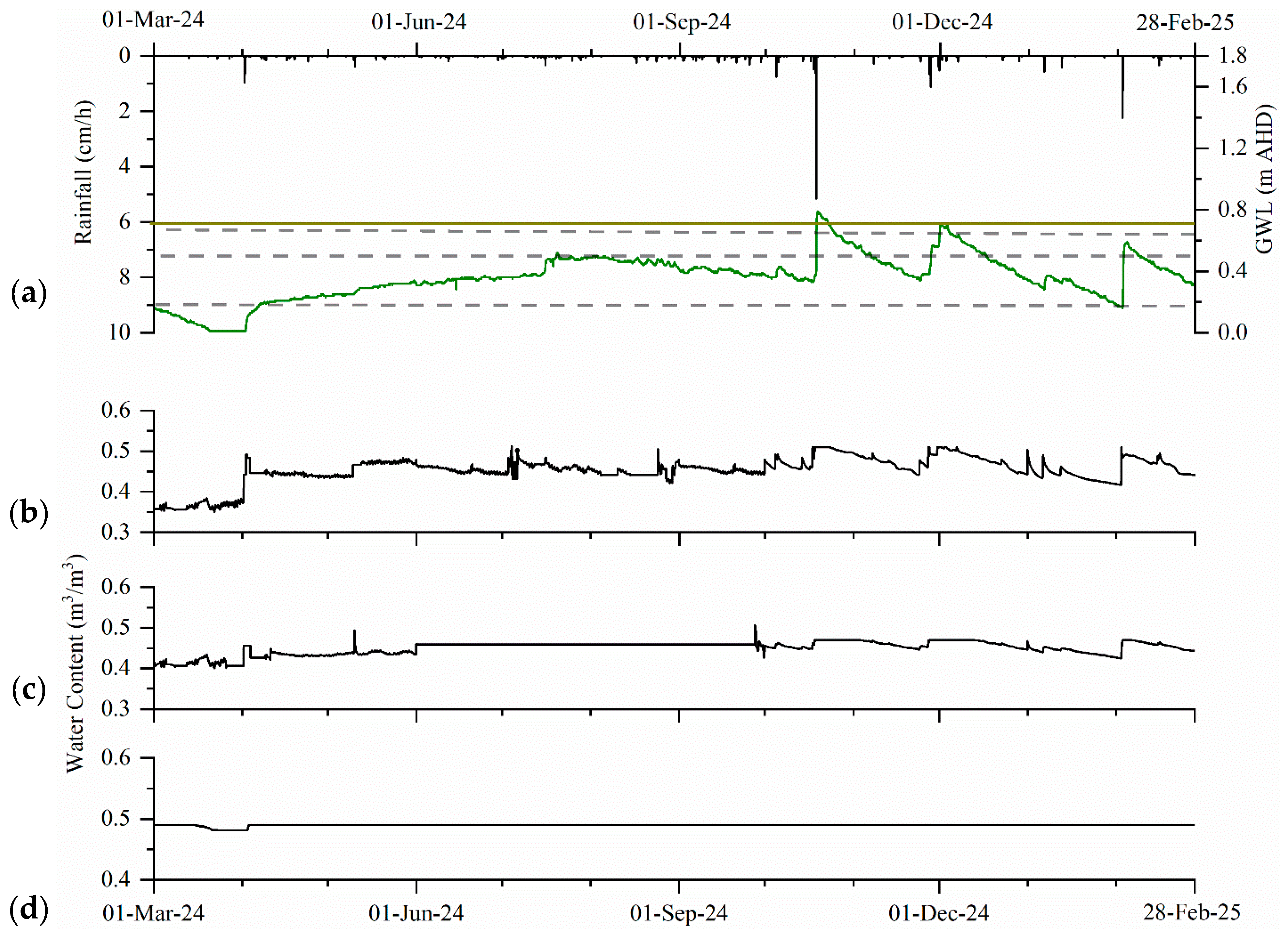
In situ water content measured at S (Figure 1) is plotted in Figure 2. As the soil is mainly clay and the groundwater table is high, capillary suction is significant, and the soil is near saturation throughout the monitoring period. The water content near the surface shows higher variability compared to the deeper layers since the surficial soil layer responds to changes in atmospheric conditions. The bottom-most layer was fully inundated throughout most of the measurement period; therefore, the water content remained relatively constant at saturation. Nevertheless, the response of the water content throughout the soil layer to larger rainfalls is evident; the 39 mm rainfall on 1 April 2024 caused the water content near the surface to rise sharply, with a moderate increase for the other two sensor locations. Between early April 2024 and mid-October 2024, rainfall was negligible, and no distinct spikes were observed in the measured water content. The major rainfall event on 18 October 2024, with a depth of 69 mm, caused a sharp increase in water content for the top two sensor locations. Similar responses of water content to rainfall can be observed for the events on 23 November 2024, 27 November 2024, and 2 February 2025 with a total rainfall of 8.6 mm, 29.4 mm, and 47.0 mm, respectively.
The response of the soil moisture sensors is typical for high groundwater table conditions. Water content in the top layer shows a greater response to rainfall events, while it decreases in the deeper layer. The bottom-most layer being at saturation, the groundwater was always above the deepest soil moisture sensor. The soil at intermediate depth exhibits combined effects of the groundwater table and rainfall, with the response to rainfall more pronounced when the groundwater table is at a lower elevation. The sensitivity of moisture conditions in the vadose zone to groundwater levels plays a role in the quantification of water balance; given that the location of the groundwater table varies throughout the year, it can also be expected that the surface storage water balance will have a seasonal dependence.

3.2. Laboratory Measurements

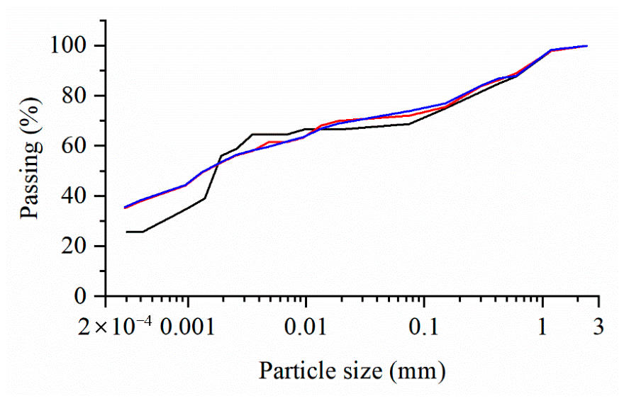
Results of the particle size distribution curves for soil samples collected on the S side at SA, SB, and SC are given in Figure 3. At the same time, Table 1 provides the results for soil texture, saturated hydraulic conductivity, bulk density, and saturated water content for the south side. Clay is the predominant soil type at S, with slight differences in the particle size distribution for samples collected at the three depths. The particle size distribution of samples collected from I1–I4, E and W (Figure 1) are provided in Figure S1, while soil properties are provided in Table S1 in the Supplementary Materials. Generally, within 100 m of N, the soil profile consisted of surficial clays (NA, NB, NC) and sandy clay loam at ND, and outside of this zone, the vadose zone consists predominantly of clays. Further details on the physical properties of the soils on the south side are given in Table S2.

3.3. Model Results

3.3.1. Water Content

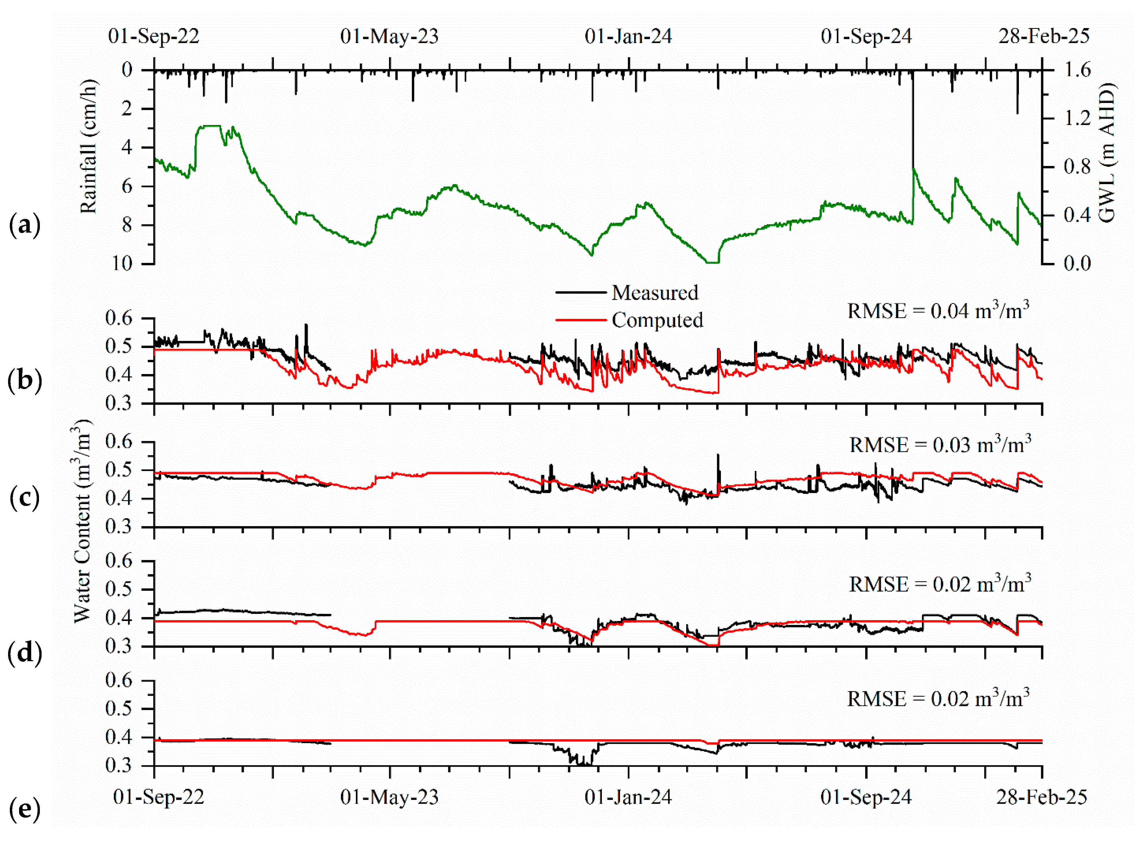
The final set of van Genuchten parameters is provided in Table 2. The van Genuchten parameter values obtained from the current experiments were averaged with the values for the N side obtained from the previous study. The averaged parameter set was adopted to run the HYDRUS-2D model. The simulated water content for the N side is consistent with that obtained from the previous HYDRUS-1D simulations [35], and as shown in Figure 4, the agreement between model results and field data is good, with the RMSE varying between 0.02 and 0.04 (m3/m3) for the four soil layers (NA, NB, NC and ND, Figure 1b).
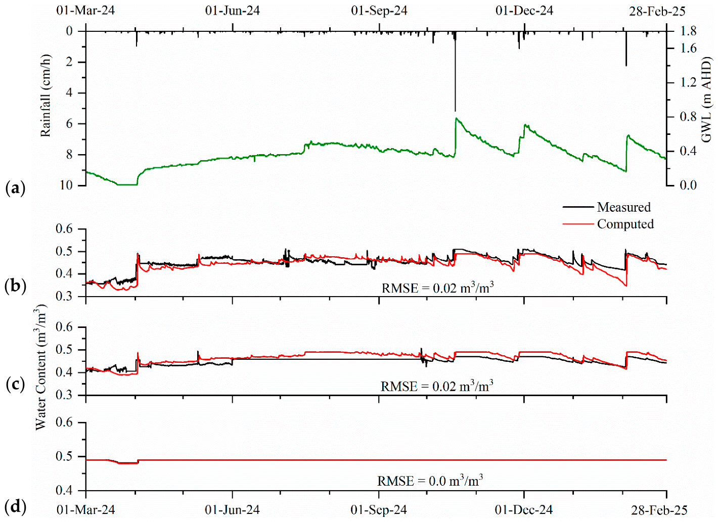
A comparison of measured and HYDRUS-2D modelled water content for the S side is shown in Figure 5. The modelled water content matches well with the measurements, with an RMSE value close to 0.02 m3/m3 in the top two layers. The soil layer at the bottom sensor location was fully saturated, and the measured and modelled water content were at saturation levels (θs = 0.38). Although measurements of rainfall, groundwater level and soil water content exhibited diverse interactions, the model was able to capture this complexity with good accuracy. The average measured water content during this period was 0.44 m3/m3 for the top layer, while the average computed water content was 0.43 m3/m3. For the second layer, the average measured and computed water contents were 0.45 and 0.46 (m3/m3), respectively.

3.3.2. Surface Water Level

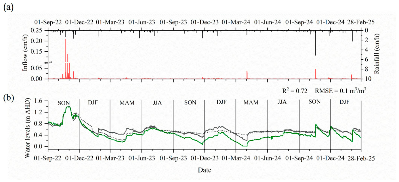
A comparison of the measured and HYDRUS-2D modelled surface water levels in the wetland is given in Figure 6. Inflow data were obtained from simulations reported in Teang et al.’s work [36]. The model can predict the surface water level with reasonable accuracy; the average modelled surface water level for the simulation period was 0.57 m AHD, similar to the measured value. The RMSE value was 0.1 m, and the R2 value was 0.72, consistent with Cannavo et al. [26] who modelled water depth in HYDRUS-2D and reported an RMSE of 0.085 m and an R2 of 0.79. Rayburg and Thoms [14] used a coupled approach consisting of satellite imagery, hydrologic and hydraulic modelling to predict the wetland inundation extent with an RMSE of less than 5% (of full volume). The surface water levels computed for three surface nodes (Figure 1b), in Z1, Z2, and Z3, consistent with the wetting and drying conditions for the three different zones, were similar, indicating that the appropriate boundary conditions were applied.
The wetland experienced contrasting hydrological conditions over the simulation period. Inflows corresponding to rain events occurring in January 2023, February 2023, April 2023, November 2023, April 2024, October 2024, December 2024 and February 2025 resulted in surface water levels rising sharply, followed by a gradual decrease after the cessation of inflow. During dry periods, surface water levels decrease in accordance with infiltration and evaporation rates. Groundwater levels increase and decrease, corresponding with recharge during rain events and dry periods, respectively. In general, our modelling results indicate a very good agreement with the measurements featuring sharp increases followed by a decrease in the surface water elevation, consistent with observations. The last quarter of 2022 experienced above-average rainfall, with the groundwater table rising above the ground surface and surface water levels reaching 1.4 m AHD. The model can reproduce this event well, with good agreement of the rising and falling phases and the peak water level.
The hydrology of Sparrovale is primarily impacted by inflow events and movements of the groundwater table, which fluctuate distinctly according to season. The model simulation period spans 30 months or ten seasons, including three (2022, 2023, 2024) spring and summer seasons and two (2023, 2024) autumn and summer seasons, allowing seasonal behaviour to be inferred. Most of the rainfall in the region occurs over the winter (JJA) and spring (SON) seasons, and groundwater elevations during these periods are higher. During the winter and spring seasons, groundwater levels can rise close to the ground surface, as is evidenced by the floods in October 2022 and data for July 2023 and October 2024. During this period, although the wetland receives inflow only from Horseshoe Bend, surface water levels in the wetland are typically higher. The shallow groundwater table induces saturation conditions in the surficial soils, diminishing soil storage and infiltration rates. As evaporation rates during the winter and spring seasons are also low, overall abstractions from surface storage are reduced significantly. Further discussions in this regard are provided in Section 3.3.3.
The surface water levels show a decreasing trend in all three summer seasons studied. The higher surface water levels in the spring season gradually decline in summer, in spite of inflows from the Balog Channel, which is in operation during this period. There is less rainfall in summer, and groundwater levels are therefore declining, increasing vadose zone thickness. Although storage in the vadose zone increases, it is still limited since soil moisture is close to saturation, as capillary suction effects of the clay soils are significant. Evaporation rates are substantial, owing to the higher temperatures, presumably accounting for the abstractions from surface storage (see Section 3.3.3). Average surface water levels are observed in the autumn months (MAM). Data for the 2023 and 2024 autumn periods do not reveal significant decreasing or increasing trends in both groundwater and surface water elevations. Autumn is generally associated with moderate rainfall, and with temperatures decreasing, evaporative losses are reduced, thereby supporting sustained water levels in the wetland.

3.3.3. Water Balance

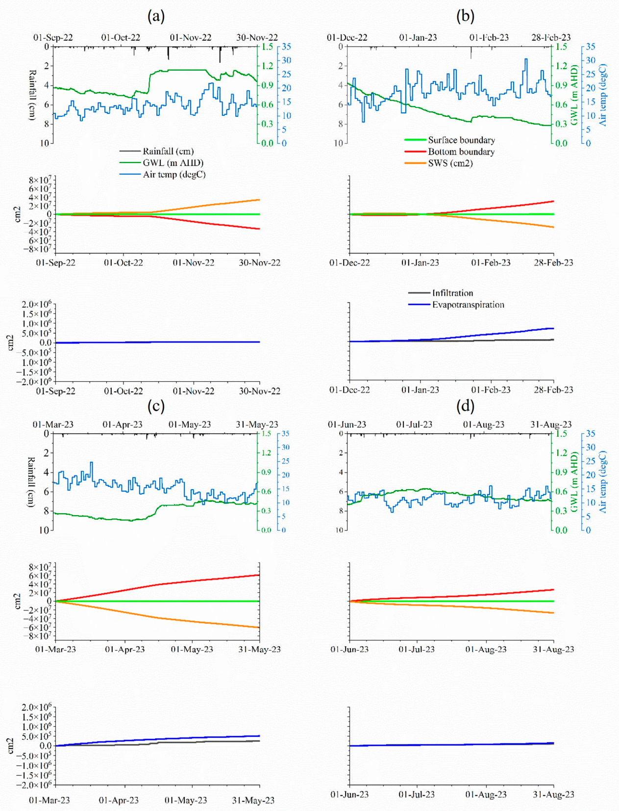
The model results were divided into ten 3-month time periods to understand the water balance behaviour at a seasonal time scale. To understand this, the net cumulative fluxes of infiltration and evapotranspiration across the ground surface (surface boundary flux) and bottom boundary and the change in soil water storage (SWS) over the individual time periods are analysed. Results for the first four seasons of the study period are given in Figure 7, while results for other seasons are provided in Figure S2 in the Supplementary Materials. In general, Figure 7 shows that the bottom boundary flux is balanced with the change in storage. This balance is generally observed for all seasons, indicative of the role of the shallow groundwater table and the impact of capillary rise; suction pressure for clays is generally high and can reach 1 m [37], contributing significantly to overall moisture balance in the vadose zone of shallow groundwater systems. On the other hand, the contribution of infiltration and evaporation at the soil surface is relatively insignificant (2 orders of magnitude less) to the overall balance, compared to the bottom boundary fluxes.
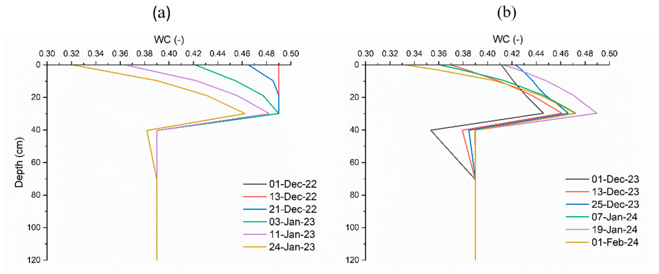
The overall moisture redistribution behaviour is evidenced from the profiles of water content shown in Figure 8a,b, for the summer (DJF) season, where decreasing and increasing groundwater table movements were experienced for 2022/23 and 2023/24 seasons, respectively. Figure 8a shows that the top 40 cm of the soil layer experience water loss due to the net effects of decreasing water table and evaporation and infiltration occurring at the surface. When the water table is rising (Figure 8b), the opposite occurs, with an increase in the moisture content in the upper soil layer due to capillary rise. Regardless of season, change to water storage in the vadose zone is met by groundwater movement and capillary effects, with evaporation and infiltration at the surface playing a less significant role in the overall moisture balance. Moisture dynamics for the same period as in Figure 8 are provided for the south side in Figure S3 in the Supplementary Materials.
At a seasonal scale, the spring season from 1 September 2022 to 30 November 2022 was exceptionally wet, with a total rainfall of 28.3 cm recorded. The wetland was flooded in November, and the average groundwater level during this season was 0.94 m AHD. The average temperature was 13.6 °C (Figure 7a). Significantly, the direction of the bottom boundary flux for 2022 (Figure 7a) is reversed compared to the 2023 and 2024 spring seasons (Figure S2, Supplementary Materials). Extensive flooding occurred during the spring of 2022, resulting in fully saturated and thus Darcy flow conditions, which reversed the flow direction across the bottom boundary. This, however, is an exceptional case and happens only during extreme flood conditions. The average temperature during the summer season (December 2022 to February 2023) was 18.8 °C, the average groundwater level was 0.47 m AHD, with total rainfall of 7.6 cm. During this season, temperatures were higher than in the spring season, groundwater levels decreased throughout the season, and evapotranspiration dominated the moisture loss at the surface with higher values than the infiltration (Figure 8). Flux at the bottom boundary is consistent with capillary rise. The average temperature during the autumn season (March 2023 to May 2023) was 15.4 °C, the average groundwater level was 0.30 m AHD, and total rainfall was 11.6 cm. The groundwater level did not depict considerable variability, and evapotranspiration led to major water losses during this season, compared to the infiltration. While evapotranspiration was higher than infiltration, it was less than the summer evapotranspiration owing to the prevalence of mild environmental conditions. During the winter season (June 2023 to August 2023), the average temperature was 11.4 °C, the average groundwater level was 0.54 m AHD, and the total rainfall was 9.7 cm. Groundwater levels did not depict a considerable variability, and evapotranspiration led to the major water losses during this season as well, as compared to the infiltration. While evapotranspiration was higher than infiltration, it was less than the summer evapotranspiration owing to the prevalence of mild environmental conditions.
The Sparrovale Wetland has no dedicated outlet for continuous outflow, and losses from surface storage are limited to evapotranspiration and infiltration. Infiltration plays a minor role as the groundwater levels are shallow in the Sparrovale Wetland, and soil water storage is at its capacity throughout the year, except for the summer season when groundwater levels decrease, increasing storage. The major water losses in the wetland, however, occur through evapotranspiration, the magnitude of which depends on atmospheric demand driven by seasonal atmospheric conditions.

4. Conclusions

The HYDRUS 2D model was successfully developed to ascertain the water balance in the Sparrovale Wetland. Extensive determination of soil physical properties helped develop a reliable model accounting for the spatial heterogeneity of soil types in the wetland, which was successfully verified against the in situ measurements. Model performance was in line with the performance of the previously developed HYDRUS 1D model. It was concluded from the results of this study that evapotranspiration plays a key role in water loss from the wetland, while infiltration has a negligible role compared to evapotranspiration. Overall, hydrological dynamics in the Sparrovale Wetland were substantially impacted by the variable groundwater levels. Flooding (or high water levels) seems to prevail in the Sparrovale Wetland almost every year (not to the magnitude of flooding in late 2022, which was an exceptional case), in or around the spring season, and the groundwater is one of the key factors behind these flooding events, alongside rainfall and inflow. Being a coastal wetland, groundwater has a higher amount of salinity in it as well, and as the groundwater interacts with the surface, salinization is expected to exacerbate as well. Soil water storage is shown to decrease, with sharply declining groundwater levels in all seasons analyzed in this study, except for the spring of 2022, when extraordinary flooding (water levels higher than 1.2 m AHD) occurred in the wetland, inundating the entire surface. This study would be helpful to the environmental management authorities of the Sparrovale Wetland. In situ measurement-based determination of van Genuchten parameters and their comparisons with modelled parameters might prove beneficial for other modelling locations with similar physical characteristics and soil types to this study. The modelling results of this study on how excess water is being processed in the Sparrovale Wetland have the potential to serve as a reference for assessing the treatment capacity of other similar nature-based solutions.

Supplementary Materials

The following supporting information can be downloaded at: https://www.mdpi.com/article/10.3390/hydrology13060139/s1. Figure S1: Particle size distribution for soil layers in the Sparrovale Wetland; Figure S2: Seasonal dynamics of water balance and environmental variables in the Sparrovale Wetland; Figure S3: Soil moisture profile for the south side during (a) declining (2022–2023, DJF) and (b) rising (2023–2024, DJF) groundwater table conditions; Table S1: Laboratory measurements of soil properties; Table S2: Mean and standard deviation (SD) of soil properties from laboratory measurements for the south side of the wetland.

Author Contributions

M.U.: conceptualization, investigations, data curation, software, validation, visualization, formal analysis, methodology, funding acquisition, writing—original draft, writing—review and editing. L.H.C.C.: methodology, investigations, visualization, validation, formal analysis, conceptualization, writing—review and editing, supervision, funding acquisition. K.N.I.: methodology, investigations, formal analysis, visualization, validation conceptualization, writing—review and editing, supervision. L.T.: validation, visualization, writing—review and editing. All authors have read and agreed to the published version of the manuscript.

Funding

This research was funded by the city of greater Geelong, Australia.

Data Availability Statement

Data availability is subject to approval. Data requests can be submitted to authors who will then seek approval from the data owners. Upon successful approval, data will be shared.

Acknowledgments

Deakin University’s award of a Deakin University Postgraduate Research Scholarship (DUPRS) for PhD studies is gratefully acknowledged by the first author. The authors are also grateful to the City of Greater Geelong for providing project funding through the project Sparrovale Wetlands Water Monitoring and Modelling Project. We also thank Donna Smithyman (City of Greater Geelong) and Jarrod Gaut (WaterInsites (VIC) Pty Ltd., Geelong, Australia.) for the many discussions over the course of this project, and whose insightful comments have made an immense contribution to the study.

Conflicts of Interest

The authors declare no conflicts of interest.

References

  1. Walsh, C.J.; Roy, A.H.; Feminella, J.W.; Cottingham, P.D.; Groffman, P.M.; Morgan, R.P. The urban stream syndrome: Current knowledge and the search for a cure. J. N. Am. Benthol. Soc. 2005, 24, 706–723. [Google Scholar] [CrossRef]
  2. Jia, K.; Huang, A.; Yin, X.; Yang, J.; Deng, L.; Lin, Z. Investigating the impact of urbanization on water ecosystem services in the dongjiang river basin: A spatial analysis. Remote Sens. 2023, 15, 2265. [Google Scholar] [CrossRef]
  3. Chocat, B.; Ashley, R.; Marsalek, J.; Matos, M.R.; Rauch, W.; Schilling, W.; Urbonas, B. Toward the sustainable management of urban storm-water. Indoor Built Environ. 2007, 16, 273–285. [Google Scholar] [CrossRef]
  4. Lane, C.R.; Leibowitz, S.G.; Autrey, B.C.; LeDuc, S.D.; Alexander, L.C. Hydrological, physical, and chemical functions and connectivity of non-floodplain wetlands to downstream waters: A review. JAWRA J. Am. Water Resour. Assoc. 2018, 54, 346–371. [Google Scholar] [CrossRef] [PubMed]
  5. Robinson, A.E.; Scaini, A.; Peña, F.J.; Hambäck, P.A.; Humborg, C.; Jaramillo, F. The hydrological archetypes of wetlands. Hydrol. Earth Syst. Sci. 2025, 29, 5975–6001. [Google Scholar] [CrossRef]
  6. Ferguson, B.K. Role of the long-term water balance in management of stormwater infiltration. J. Environ. Manag. 1990, 30, 221–233. [Google Scholar] [CrossRef]
  7. Cartwright, N.; Nielsen, P.; Perrochet, P. Influence of capillarity on a simple harmonic oscillating water table: Sand column experiments and modeling. Water Resour. Res. 2005, 41, W08416. [Google Scholar] [CrossRef]
  8. Gunawardhana, M.; Treby, S.; Silvester, E.; Jones, O.A.; Grover, S. Sphagnum peatland hydrological balance shows high groundwater dependence and resilience to short-term dry periods. Water Resour. Res. 2025, 61, e2024WR039454. [Google Scholar] [CrossRef]
  9. Kong, J.; Xin, P.; Hua, G.F.; Luo, Z.Y.; Shen, C.J.; Chen, D.; Li, L. Effects of vadose zone on groundwater table fluctuations in unconfined aquifers. J. Hydrol. 2015, 528, 397–407. [Google Scholar] [CrossRef]
  10. Li, L.; Barry, D.A.; Stagnitti, F.; Parlange, J.Y.; Jeng, D.S. Beach water table fluctuations due to spring–neap tides: Moving boundary effects. Adv. Water Resour. 2000, 23, 817–824. [Google Scholar] [CrossRef]
  11. Raisin, G.; Bartley, J.; Croome, R. Groundwater influence on the water balance and nutrient budget of a small natural wetland in Northeastern Victoria, Australia. Ecol. Eng. 1999, 12, 133–147. [Google Scholar] [CrossRef]
  12. Wallace, J.; Nicholas, M.; Grice, A.; Waltham, N.J. Application of a water balance model using depth measurements in the Mungalla wetland in north Queensland, Australia. J. Hydrol. 2024, 644, 132055. [Google Scholar] [CrossRef]
  13. Chen, S.; Johnson, F.; Drummond, C.; Glamore, W. A new method to improve the accuracy of remotely sensed data for wetland water balance estimates. J. Hydrol. Reg. Stud. 2020, 29, 100689. [Google Scholar] [CrossRef]
  14. Rayburg, S.; Thoms, M. A coupled hydraulic–hydrologic modelling approach to deriving a water balance model for a complex floodplain wetland system. Hydrol. Res. 2009, 40, 364–379. [Google Scholar] [CrossRef]
  15. Sun, G.; Saeed, T.; Zhang, G.; Sivakugan, N. Water quantity and quality assessment on a tertiary treatment wetland in a tropical climate. Water Sci. Technol. 2015, 71, 511–517. [Google Scholar] [CrossRef]
  16. Yihdego, Y.; Webb, J.A. Assessment of wetland hydrological dynamics in a modified catchment basin: Case of Lake Buninjon, Victoria, Australia. Water Environ. Res. 2017, 89, 144–154. [Google Scholar] [CrossRef] [PubMed]
  17. Gilfedder, B.S.; Frei, S.; Hofmann, H.; Cartwright, I. Groundwater discharge to wetlands driven by storm and flood events: Quantification using continuous Radon-222 and electrical conductivity measurements and dynamic mass-balance modelling. Geochim. Cosmochim. Acta 2015, 165, 161–177. [Google Scholar] [CrossRef]
  18. Sadat-Noori, M.; Anibas, C.; Andersen, M.S.; Glamore, W. A comparison of radon, heat tracer and head gradient methods to quantify surface water-groundwater exchange in a tidal wetland (Kooragang Island, Newcastle, Australia). J. Hydrol. 2021, 598, 126281. [Google Scholar] [CrossRef]
  19. Krasnostein, A.L.; Oldham, C.E. Predicting wetland water storage. Water Resour. Res. 2004, 40, W10203. [Google Scholar] [CrossRef]
  20. Goutaland, D.; Winiarski, T.; Lassabatere, L.; Dubé, J.S.; Angulo-Jaramillo, R. Sedimentary and hydraulic characterization of a heterogeneous glaciofluvial deposit: Application to the modeling of unsaturated flow. Eng. Geol. 2013, 166, 127–139. [Google Scholar] [CrossRef]
  21. Winiarski, T.; Lassabatere, L.; Angulo-Jaramillo, R.; Goutaland, D. Characterization of the heterogeneous flow and pollutant transfer in the unsaturated zone in the fluvio-glacial deposit. Procedia Environ. Sci. 2013, 19, 955–964. [Google Scholar] [CrossRef]
  22. Nimmer, M.; Thompson, A.; Misra, D. Modeling water table mounding and contaminant transport beneath storm-water infiltration basins. J. Hydrol. Eng. 2010, 15, 963–973. [Google Scholar] [CrossRef]
  23. Cook, F.J.; Rassam, D.W. An analytical model for predicting water table dynamics during drainage and evaporation. J. Hydrol. 2002, 263, 105–113. [Google Scholar] [CrossRef]
  24. Slimene, E.B.; Lassabatere, L.; Winiarski, T.; Gourdon, R. Modeling water infiltration and solute transfer in a heterogeneous vadose zone as a function of entering flow rates. J. Water Resour. Prot. 2015, 7, 1017–1028. [Google Scholar] [CrossRef][Green Version]
  25. Wang, G.T.; Chen, S.; Barber, M.E.; Yonge, D.R. Modeling flow and pollutant removal of wet detention pond treating stormwater runoff. J. Environ. Eng. 2004, 130, 1315–1321. [Google Scholar] [CrossRef]
  26. Cannavo, P.; Coulon, A.; Charpentier, S.; Béchet, B.; Vidal-Beaudet, L. Water balance prediction in stormwater infiltration basins using 2-D modeling: An application to evaluate the clogging process. Int. J. Sediment Res. 2018, 33, 371–384. [Google Scholar] [CrossRef]
  27. Locatelli, L.; Mark, O.; Mikkelsen, P.S.; Arnbjerg-Nielsen, K.; Deletic, A.; Roldin, M.; Binning, P.J. Hydrologic impact of urbanization with extensive stormwater infiltration. J. Hydrol. 2017, 544, 524–537. [Google Scholar] [CrossRef]
  28. Shahzad, H.; Myers, B.; Boland, J.; Hewa, G.; Johnson, T. Stormwater runoff reduction benefits of distributed curbside infiltration devices in an urban catchment. Water Res. 2022, 215, 118273. [Google Scholar] [CrossRef] [PubMed]
  29. Birch, G.F.; Fazeli, M.S.; Matthai, C. Efficiency of an infiltration basin in removing contaminants from urban stormwater. Environ. Monit. Assess. 2005, 101, 23–38. [Google Scholar]
  30. Bonneau, J.; Fletcher, T.D.; Costelloe, J.F.; Poelsma, P.J.; James, R.B.; Burns, M.J. The hydrologic, water quality and flow regime performance of a bioretention basin in Melbourne, Australia. Urban Water J. 2020, 17, 303–314. [Google Scholar] [CrossRef]
  31. Bonneau, J.; Fletcher, T.D.; Costelloe, J.F.; Poelsma, P.J.; James, R.B.; Burns, M.J. Where does infiltrated stormwater go? Interactions with vegetation and subsurface anthropogenic features. J. Hydrol. 2018, 567, 121–132. [Google Scholar] [CrossRef]
  32. Boratto, D.; Kurylyk, B.L.; Jamieson, R. Modeling a rapid infiltration basin for wastewater treatment in the Arctic under various operating conditions. J. Contam. Hydrol. 2025, 273, 104601. [Google Scholar] [CrossRef] [PubMed]
  33. Clozel, B.; Ruban, V.; Durand, C.; Conil, P. Origin and mobility of heavy metals in contaminated sediments from retention and infiltration ponds. Appl. Geochem. 2006, 21, 1781–1798. [Google Scholar] [CrossRef]
  34. El-Mufleh, A.; Béchet, B.; Ruban, V.; Legret, M.; Clozel, B.; Barraud, S.; Gonzalez-Merchan, C.; Bedell, J.P.; Delolme, C. Review on physical and chemical characterizations of contaminated sediments from urban stormwater infiltration basins within the framework of the French observatory for urban hydrology (SOERE URBIS). Environ. Sci. Pollut. Res. 2014, 21, 5329–5346. [Google Scholar] [CrossRef] [PubMed]
  35. Usman, M.; Chua, L.H.; Irvine, K.N.; Teang, L. Numerical modelling of vadose zone flow for a shallow groundwater wetland using HYDRUS-1D. Model. Earth Syst. Environ. 2025, 11, 296. [Google Scholar] [CrossRef]
  36. Teang, L.; Irvine, K.N.; Chua, L.H.; Usman, M. Dynamics of Runoff Quantity in an Urbanizing Catchment: Implications for Runoff Management Using Nature-Based Retention Wetland. Hydrology 2025, 12, 141. [Google Scholar] [CrossRef]
  37. Guymon, G.L. Unsaturated Zone Hydrology; Prentice Hall (Pearson Education): Englewood Cliffs, NJ, USA, 1994. [Google Scholar]
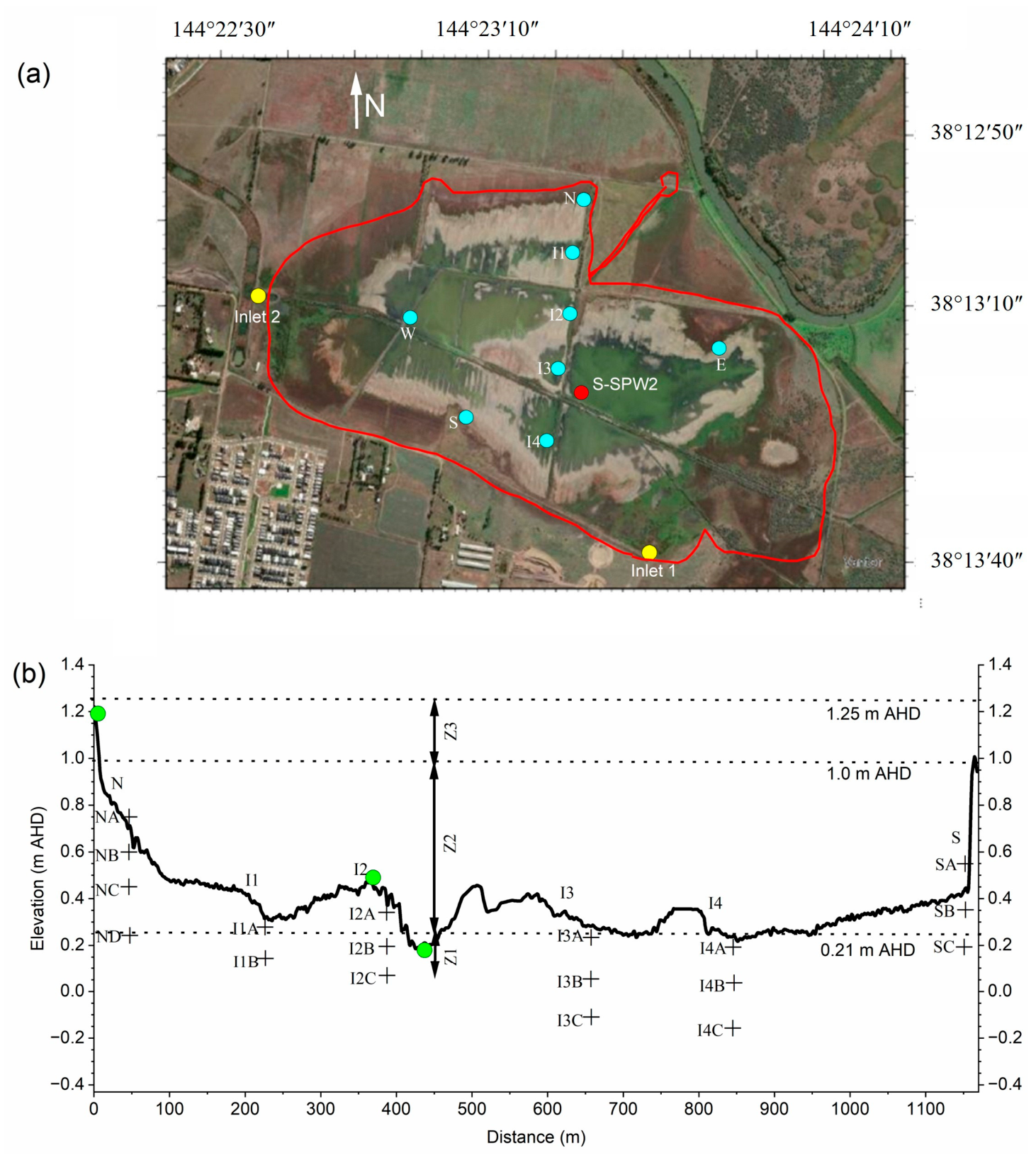
Figure 1. Location of (a) Sparrovale Wetland. N, I1, … I4, S, E., W (cyan color) represent soil sampling locations for the current study. The red line denotes the boundary of the Sparrovale Wetland. (b) The black line from left to right represents the surface elevation across the Sparrovale Wetland. Z1, Z2, and Z3 represent zones of permanent surface wetting, periodic surface wetting and drying, and a permanently dry surface, respectively. Green dots represent the observation nodes for model validation, and “+” symbol indicates locations where soil samples were obtained. S-SPW2 is the location of the surface water monitor [35].
Hydrology 13 00139 g001
Figure 2. In situ measurements of water content at S. (a) Rainfall, groundwater elevation (green line) and soil moisture sensor locations (dashed lines) and measured moisture content in soil layers (b) SA, (c) SB, and (d) SC. The pale green line represents the ground surface elevation.
Hydrology 13 00139 g002
Figure 3. Particle size distribution for soil layers at S. Black, red, and blue lines represent layers SA, SB, and SC, respectively.
Hydrology 13 00139 g003
Figure 4. (a) Rainfall (black bars), groundwater elevation (green line). Measured and computed water content for: (b) NA, (c) NB, (d) NC and (e) ND, respectively.
Hydrology 13 00139 g004
Figure 5. (a) Rainfall (black bars), groundwater elevation (green line). Measured and computed water content for: (b) SA, (c) SB, and (d) SC, respectively.
Hydrology 13 00139 g005
Figure 6. (a) Measured rainfall (black bars) and inflow (red bars) [36]. (b) Measured groundwater levels (green) measured (solid black line) and computed (dotted black line) surface water levels. SON represents spring, DJF represents summer, MAM represents autumn, and JJA represents winter.
Hydrology 13 00139 g006
Figure 7. Rainfall, groundwater level, cumulative fluxes across the ground surface and bottom boundary, soil water storage, evaporation and infiltration. (a) Spring (1 September 2022 to 30 November 2022), (b) summer (1 December 2022 to 28 February 2023), (c) autumn (1 March 2023 to 31 May 2023), and (d) winter (1 June 2023 to 30 August 2023).
Hydrology 13 00139 g007
Figure 8. Soil moisture profile for the north side during (a) declining (2022–2023, DJF) and (b) rising (2023–2024, DJF) groundwater table conditions.
Hydrology 13 00139 g008
Table 1. Laboratory measurements of soil properties.
Soil LayerDepth (cm)Sand (%)Silt (%)Clay (%)Soil
Texture
ρb (g/cm3)Ks
(cm/Day)
θs
(m3/m3)
SA20231562Clay1.3 ± 0.111.4 ± 0.60.50 ± 0.01
SB40241957Clay1.2 ± 0.114.2 ± 0.80.48 ± 0.01
SC60231859Clay1.3 ± 0.113.2 ± 1.10.48 ± 0.01
Table 2. Final values of van Genuchten parameters used to run the HYDRUS-2D model.
Soil Textureθr (–)θs (–)α (1/cm)n (–)Ks (cm/hr)
Clay0.10.490.031.260.55
Sandy clay loam0.010.390.031.450.79
Disclaimer/Publisher’s Note: The statements, opinions and data contained in all publications are solely those of the individual author(s) and contributor(s) and not of MDPI and/or the editor(s). MDPI and/or the editor(s) disclaim responsibility for any injury to people or property resulting from any ideas, methods, instructions or products referred to in the content.