The Contribution of Natural Isotopes in Understanding Groundwater Circulation: Case Studies in Carbonate Aquifers of Central Apennines

Abstract

Groundwater quantification is essential for sustainable water resources management, yet it is often hampered by limited data availability and difficulties in measuring spring discharges. This study investigates three carbonate aquifers in Central Italy’s Abruzzo region: the Genzana–Greco, Morrone, and Marsicano mountains. The aim is to resolve uncertainties in spring attribution, and groundwater flow patterns using isotopic analyses combined with field surveys. The Genzana–Greco aquifer was examined to clarify the sources of the Acquachiara spring and the previously unreported Germina spring, assessing whether recharge occurs locally or from the carbonate massif. In this case, the results indicate that the Germina, together with a similar known spring of Capolaia, share a common recharge sector, while the Acquachiara spring is mainly fed by higher-elevation carbonate areas, excluding significant contributions from local alluvial deposits. In the Morrone mountain aquifer, discharge gains along the Pescara River through the Gole di Popoli were quantified, and spring isotopic compositions were compared to the main basal spring Giardino to better define groundwater contributions. In this case study, the stable isotopes and tritium data confirm recharge from the central–southern massif and support the identification of basal springs and Pescara River gains as primary discharge points, with minimal influence from surface water. For the Marsicano mountain aquifer, the role of Lake Scanno in feeding the Villalago springs was investigated through isotopic analysis of inflows, downstream springs, and basal aquifer discharge points to constrain the hydrogeological water budget. The results highlight Lake Scanno’s role in the recharge of Villalago springs and delineate the Cavuto group as a major discharge system receiving inputs from central and northern sectors of the massif. Overall, the integration of isotopic tracers with hydrological measurements allowed a more precise characterization of aquifer recharge areas, Mean Residence Times, and groundwater flow paths, improving the understanding of regional water resources in a complex carbonate setting.

1. Introduction

Accurate quantification of groundwater is critical for the sustainable management of water resources; however, it remains a significant challenge due to the limited availability of hydrogeological data for regional aquifers and the intrinsic difficulties associated with accurately measuring spring discharge.

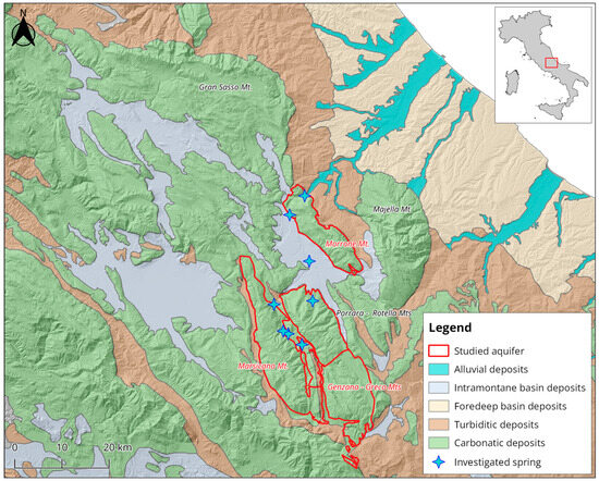
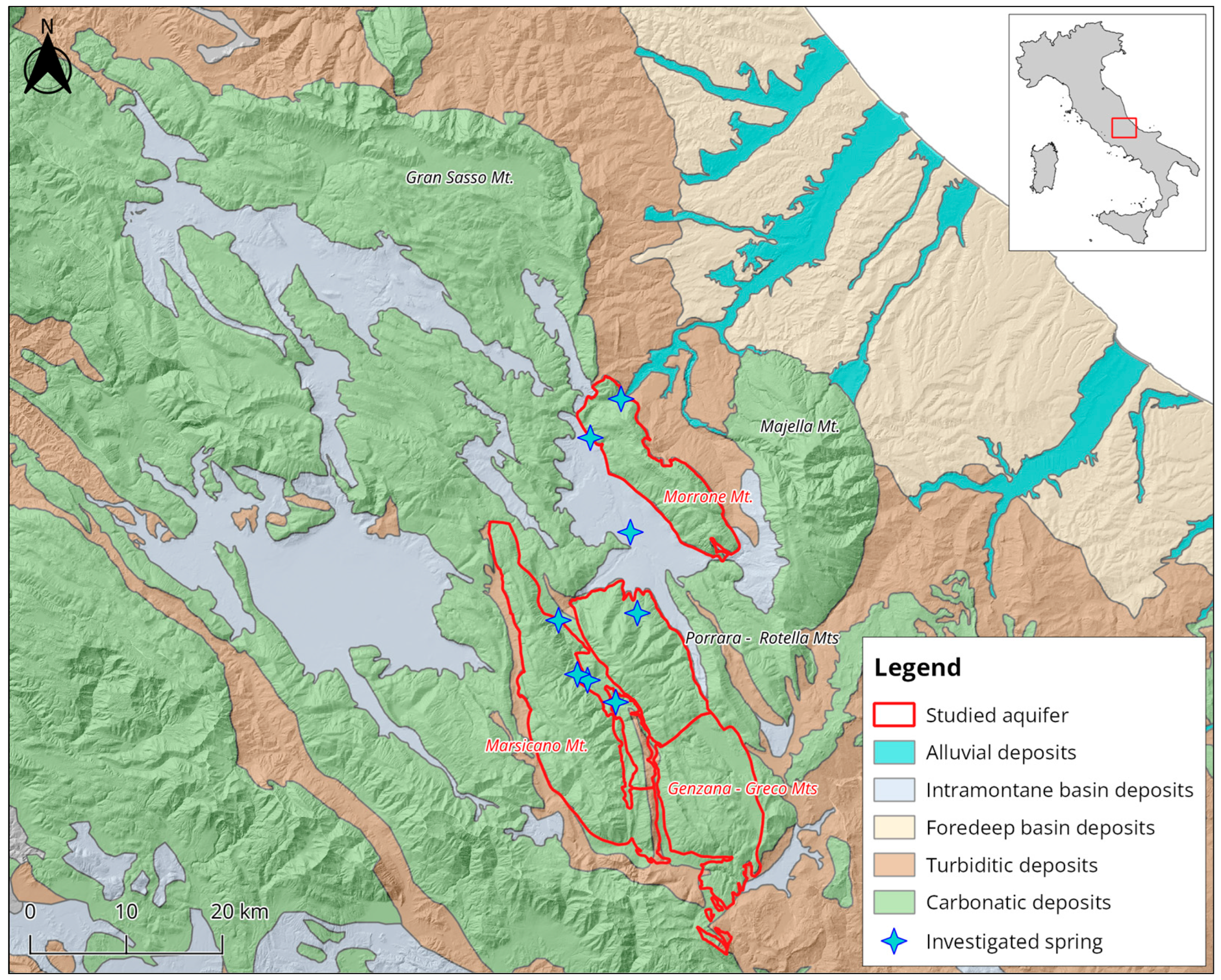
In Central Italy, the main aquifers are located within the major carbonate massifs [1,2,3], characterized by a large number of basal springs, many of which are exploited for drinking water supply [4,5,6] (Figure 1). Within the study area, three aquifers were investigated to address the uncertainties concerning spring attribution and groundwater flow patterns, the Genzana–Greco mountains’ aquifer, the Morrone mountain, and the Marsicano mountain’s ones.

Isotopic analyses of Oxigen18, Deuterium, and Tritium, combined with field surveys, were used to address the existing uncertainties. Some isotopic characterizations are available in previous works [7,8,9,10], but none of them fully resolve the questions concerning the aquifers mentioned above.

Similar approaches have been applied in numerous case studies of carbonate aquifers worldwide [11,12,13,14,15,16,17]. At the local scale, the multidisciplinary isotopic approach, beyond the studies already cited [7,8,9,10], has also been explored in investigations of the Gran Sasso carbonate aquifer [18,19] and the central Apennines [20,21].

This study utilized isotopic data from two seasonal surveys conducted within the framework of a research agreement funded by the Central Apennine Basin Authority (AUBAC), aimed at estimating the hydrological balance of Apennine aquifers. Accordingly, this work does not represent a comprehensive isotopic investigation involving multiple samples of numerous springs; rather, it constitutes an effort to leverage the available isotopic data from the agreement to complement the existing hydrogeological knowledge of the three aquifers, integrating both information reported in the literature and newly acquired data.

The marked lithological homogeneity and the very similar elevations among these aquifers have historically limited the ability of chemical and isotopic techniques to provide more detailed discrimination, unless complex and highly articulated artificial-tracer experiments are employed.

It must also be considered that, in additional cases, the boundaries between two or more morphologically defined units lie buried beneath lacustrine or alluvial deposits, where inter-unit hydraulic exchanges occur within these unconsolidated sediments. Such exchanges are neither visible nor directly quantifiable. This condition not only hides the actual discharge points of the units but also prevents the allocation of individual outflow components to one unit or another.

Beyond the approximations inherent in hydrological budget calculations, discharge measurements, and the wholeness of monitored outputs, the delineation of hydrogeological units as currently defined represents a necessary schematization of the regional groundwater flow system, and therefore of the associated hydrological and hydrogeological budgets.

The questions about Genzana–Greco Mts.’ aquifer were about the attribution of the Acquachiara spring to it and the characterization of a tapped spring (Germina), detected during field surveys and previously unreported in the literature.

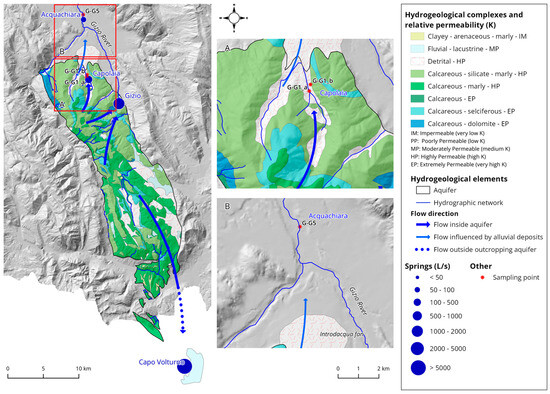
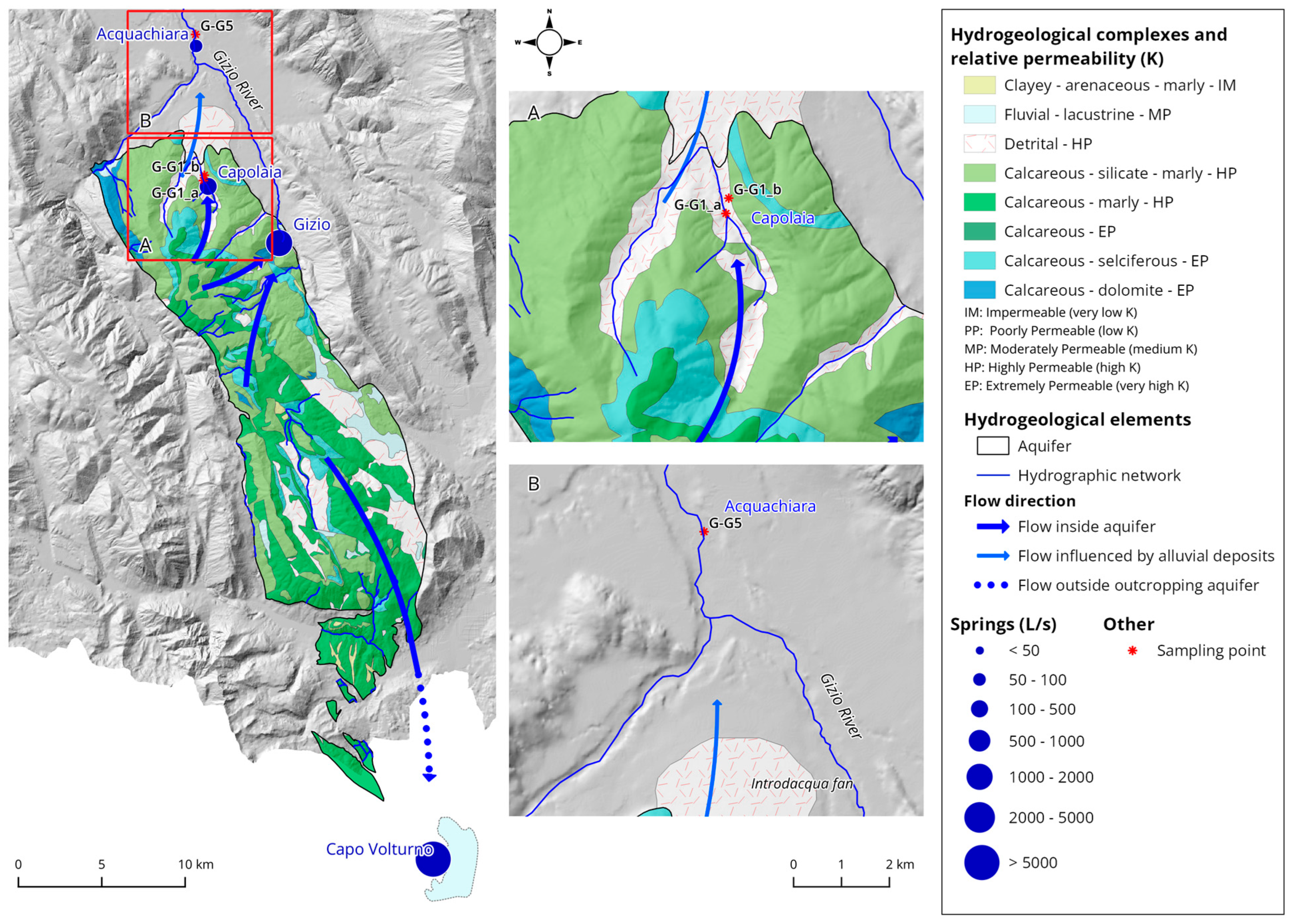
Despite emerging within the Sulmona plain, the Acquachiara spring has been attributed—based on hydrogeological investigations [22,23] and unreferenced tracer tests—to the Genzana–Greco aquifer and, at least in part, to the Introdacqua alluvial fan (Figure 2).

Given the substantial difference between the spring’s elevation and the mean elevation of the Genzana–Greco aquifer, isotopic analyses were considered the most suitable method for estimating the mean isotopic infiltration altitude (MIIA) and Mean Residence Time (MRT). These parameters were used to reconstruct the recharge system feeding the spring and to resolve whether it is recharged locally within the plain or by the carbonate aquifer.

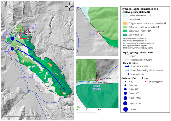
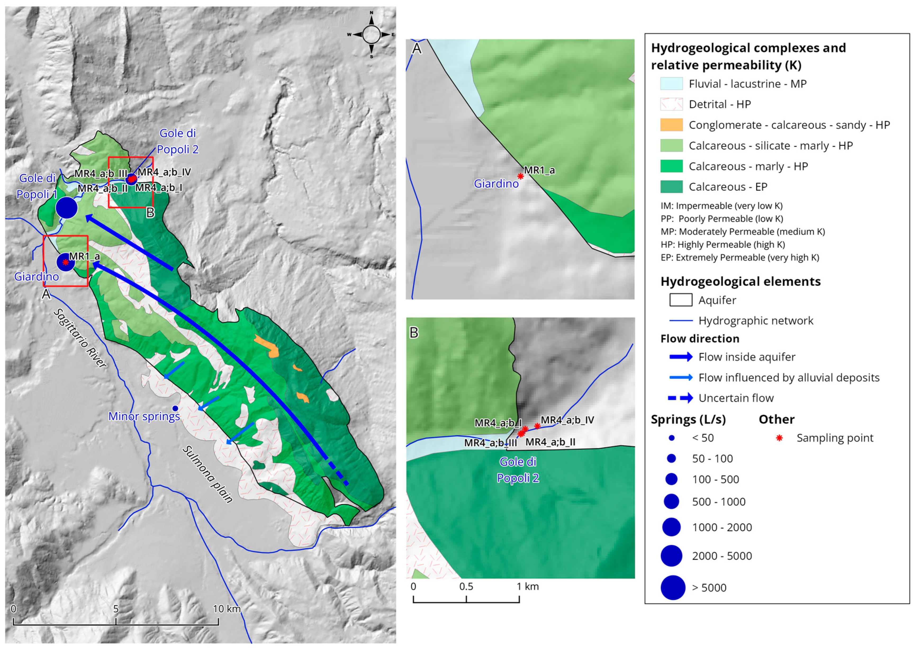
The definition and quantification of discharge gains along the Pescara River through the Gole di Popoli, belonging to the Morrone Mt. aquifer (Figure 3), although addressed in several studies [2,3,24,25,26,27,28], have always been difficult to define due to the high discharge of the Pescara River. Likewise, the assessment of water quality status required further investigation, as river water chemistry was not representative of groundwater composition. For these reasons, in addition to a more precise definition of discharge measurement sections along the gorges, spring sampling and analysis were conducted on visible springs within the gorge area. Their isotopic compositions were compared with that of the Giardino spring, which represents the main and well-defined discharge point of the groundwater body.

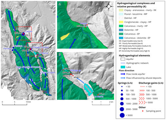
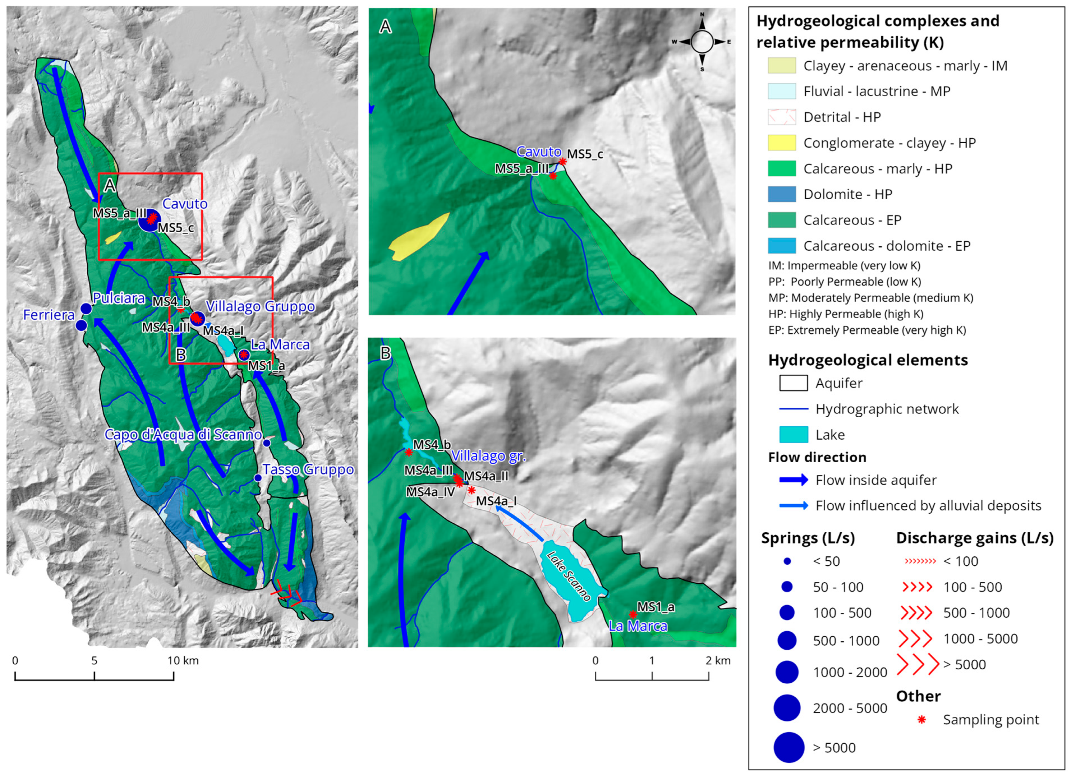
The last aquifer is the Marsicano Mt.’s one (Figure 4), where the role of Lake Scanno in the groundwater circulation feeding the Villalago springs is not clear. The presence of springs downstream of Lake Scanno has long suggested groundwater drainage from the lake, which has two inflowing streams (one of which, the La Marca spring, originates from the same aquifer), several diffuse inflow sources, and an outflow channel active only during high water stages.

In line with recent studies [9], and with the additional aim of more accurately constraining the hydrogeological water budget of the aquifer system, isotopic analyses were conducted on the La Marca inflow spring, on the springs located downstream of the lake, and on the main discharge points of the basal aquifer (Cavuto springs).

2. Materials and Methods

2.1. Study Area and Major Hydrogeological Issues

In the central Apennines of the Abruzzo region, the boundaries that define the aquifers are primarily controlled by the tectonic relationships between permeable carbonate complexes, characterized by fracturing and karstification, and terrigenous complexes, mainly turbiditic sequences composed of marly–clayey–arenaceous formations that have low permeability, as well as continental lacustrine silty–clayey deposits, which similarly show low or non-permeability.

The contacts between these complexes are embedded within elongated structural domains with an overall northwest–southeast orientation and high continuity. These structures often hinder the precise delineation of aquifers as they appear morphologically at the outcrop scale. Consequently, for some aquifers, morphological boundaries do not coincide with hydrogeological ones, which may extend beneath adjacent units. This is the case, already highlighted by Boni et al. [3], of the big aquifer, in which the authors group the Gran Sasso–Sirente Mts., Morrone Mt., Porrara–Rotella Mts., Genzana–Greco Mts., and Marsicano Mt. aquifers (Figure 1) into a single system, as hydraulic exchanges and mutual contributions cannot be excluded, nor can basal springs be located at the boundaries between different morphological units be unequivocally attributed to one aquifer or another.

In detail, the Genzana and Greco aquifer, extending over approximately 279 km², is morphologically characterized by the two homonymous mountain massifs, aligned along the Apennine structural trend. As above-mentioned, the hydrogeological boundaries [1,2,22,23] are predominantly controlled by compressional tectonic structures along the eastern slope, where the carbonate succession of the Genzana–Greco unit encounters that of near reliefs. Along this structural alignment, slices of low permeability turbiditic complexes locally occur (Figure 2).

The main springs, Gizio, Capolaia, and Acquachiara, are in the north-eastern side of the aquifer and their average discharges are 1.60 m³/s, 0.12 m³/s, and 0.70 m³/s, respectively. Another basal spring, Capo Volturno, is in the southeastern portion of the aquifer, with a discharge of about 6.6 m³/s, obtained from the literature data [29].

The Morrone Mt. aquifer extends to 107 km² and it is characterized by well-defined no-flow boundaries controlled by tectonic and stratigraphic contacts. These contacts put together fractured and karstified carbonate lithologies, with high permeability, against terrigenous and fluvio-lacustrine deposits that are low permeable or nearly impermeable.

Infiltrating waters predominantly recharge the basal aquifer, whose discharge points are located in the most depressed sectors of the carbonate ridge, like the Giardino spring (1.1 m³/s) and the Gole di Popoli group 1 (2.1 m³/s) and group 2 (~0.3 m³/s). Groundwater circulation is strongly influenced by the tectonic framework, which controls the position of the hydrogeological boundaries, the main flow paths, and the location of contact springs [24].

A secondary hydrogeological role, along the western boundary with the Sulmona plain, is played by the debris deposits, which sustain minor springs (about 21 L/s) and likely contribute to the recharge of both the plain aquifer and the Sagittario River (Figure 3).

The Marsicano Mt. aquifer (Figure 4), which extends to 234 km², is delimited by well-defined no-flow boundaries controlled by tectonic contacts [30]. Along the eastern margin, a thrust set against permeable Cretaceous–Miocene carbonates with low-permeability Miocene flysch deposits. The western and southern boundaries are defined by fault contacts between carbonate successions and Miocene flysch or turbiditic deposits.

2.2. Sampling and Isotopic Analysis

Groundwater sampling was carried out during two field campaigns at nine springs (Figure 1, Figure 2, Figure 3 and Figure 4) located in the Abruzzo Apennines, in August 2024 and May 2025.

During each campaign, a total of 18 samples were collected from the nine springs, and physico-chemical parameters were measured in the field. For each sample, two 100 mL vials and one 1 L bottle were taken. The 100 mL samples were collected for ¹⁸O and D analyses and for this reason water was filtrated; the 1 L samples for tritium, on the other side, were not.

2.2.1. δ¹⁸O–δD

The δ¹⁸O and δ²H isotopic ratios were measured at the Institute of Geosciences and Earth Resources (CNR-IGG), Via Giuseppe Moruzzi, 1, 56127 Pisa, Italy, using a Picarro L2130-i analyzer (Picarro, Inc., 3105 Patrick Henry Dr., Santa Clara, CA 95054, USA) based on cavity ring-down spectroscopy (CRDS). Results are reported in δ‰ relative to V-SMOW and calibrated to the VSMOW-SLAP scale using IAEA reference materials. Instrument performance and data quality were routinely checked by repeated measurements of internal standards and reference materials throughout the analytical sequence. The analytical precision was ±0.1‰ for δ¹⁸O and ±1‰ for δ²H.

The estimation of the mean isotopic infiltration altitude from δ¹⁸O and δD isotopic data involves defining and verifying the δ¹⁸O–δD relationship, as well as assessing the correlation between elevation and δ¹⁸O values.

The first relationship serves as a methodological check to ensure that the sampled waters belong exclusively to the active hydrological cycle and have not undergone re-evaporation processes during subsurface flow or, more generally, temperature-related fractionation capable of altering the isotopic ratio. This verification step is therefore preliminary to the estimation of mean isotopic infiltration altitude, which can be performed only if a reliable δ¹⁸O–elevation correlation line is available.

Such a correlation may be derived from meteorological observations [31] or from other isotopic datasets [8,9]. All isotopic compositions are expressed as δ values (‰) relative to VSMOW.

2.2.2. Tritium

Tritium (³H or T) is an isotope of hydrogen and the only radioactive one; it is heavier than the stable hydrogen and it is a low-energy beta emitter with a 12.31-year half-life [32]. Tritium is produced as a result of cosmic radiation through interactions with ¹⁴N, according to the reactions ¹⁴N + n → ³H + ¹²C, or ¹⁴N + n → ³H + 3α, where $n$ is a high-energy neutron associated with cosmic rays [33,34]. It becomes part of the water molecule by combining with atmospheric oxygen. Through precipitation, it enters the hydrological cycle and eventually reaches groundwater. As long as the water remains in the atmosphere, the tritium content remains constant, since it is produced at the same rate as it decays, according to the reaction ³H → ³He + β.

The application of these concepts in hydrogeology is based on the principle that, once tritium enters the subsurface as part of the water molecule, it decays and is no longer regenerated. It can therefore be used for groundwater dating, provided that the initial concentration, i.e., that of meteoric waters at the time of their infiltration into the subsurface domain, is known.

Groundwater progressively becomes depleted in tritium in accordance with its half-life; the time elapsed since infiltration—and consequently the groundwater transit time from infiltration to discharge or to the sampling location—is determined using the radioactive decay equation, which in this case is expressed as follows:

C_as = C_p e^−λt

(1)

with

C_as = tritium concentration in sampled groundwater;

C_p = tritium concentration in precipitation at the time of infiltration;

λ = tritium radioactive decay constant (equal to 0.693/T_1/2 = 0.05575 y⁻¹);

t = time in years between infiltration and analysis.

Solving the above equation for t yields:

t = (1/λ) (ln C_p − ln C_as)

(2)

The tritium concentration is expressed in TU (Tritium Units), corresponding to the presence of one tritium atom per 10¹⁸ hydrogen atoms. Atmospheric tritium levels increased significantly during the period of thermonuclear weapons testing, rising by about three orders of magnitude (approximately 3000–4000 TU in the early 1960s) compared to the natural background level. Following the ban on nuclear weapons testing, concentrations gradually decreased, reaching pre-nuclear levels (around 5–10 TU) by the early 1990s.

At present, average tritium values in the Mediterranean region and surrounding areas range from about 7 to 3 TU, depending on the season and the degree of continental influence on precipitation [35].

One of the main challenges in using tritium for groundwater dating lies in determining the initial concentration (C_p), since the time of infiltration is generally unknown. However, as more than thirty years have passed since the prohibition and atmospheric tritium levels have largely stabilized, it is now possible to estimate groundwater ages using available C_p data from research institutions and international monitoring agencies.

It should also be noted that groundwater age determinations are subject to additional uncertainties, mainly due to seasonal variations in tritium content in precipitation and to the fact that aquifers—particularly extensive ones—have storage capacities exceeding annual recharge. As a result, they contain groundwater that is infiltrated at different times. Moreover, recharge may occur both near the spring, resulting in relatively short transit times, and at greater distances, leading to longer transit times. Consequently, the calculated age does not represent the actual residence time of a specific water parcel but rather an indicative Mean Residence Time (MRT) within the aquifer [36].

The evaluation of the Mean Residence Time of groundwater within the aquifer relies on the estimation of the initial tritium content (C_p in (1) and (2)).

Table 1. Tritium values from international databases and from the literature.

Site	Altitude (m a.s.l.)	Period	Cp Values (TU)	Reference
Genova	-	1990–1995	5.5–7.2	[37]
Pisa	-	1992–1995	5.8–7.3	[37]
Simbruini Mts. (Marche Region)	1750	2000–2001	6.1	[38]
Latina (Lazio Region)	35	2000–2001	4.5	[38]
Roma DST	66	2000–2001	5.4–6.2	[38]
Marche Apennines	950	1991–2000	8.5	[39]
Marche Apennines	950	2000–2001	8.2	[39]
Marche Apennines	1200	2023–2025	4.91	*
Marche Apennines	190	2023–2025	5.97	*

* Personal communication (Tazioli A., Università Politecnica delle Marche).

summarizes several estimates provided by different authors and derived from international databases, referring to a reasonable time interval spanning approximately 1990–2010. It should be noted that, unfortunately, no updated estimates have been produced for Italy in subsequent years.

Considering the analysis periods, the morphological conditions of the sampling stations reported in Table 1, it was considered reasonable to use as terms of reference the maximum and minimum values for the entire Italian peninsula equal to 8.5 and 4.5, respectively.

Taking into account the above considerations, particularly the uncertainty associated with the estimation of C_p (the tritium concentration in precipitation at the time of infiltration), the obtained results should be interpreted only in a relative and qualitative sense and cannot be considered quantitatively. Further investigations and/or attempts to achieve greater precision are not warranted, given both the theoretical assumptions underlying the application of the method and the analytical uncertainty inherent to the technique. The standard deviations of the analyses range from 0.2 to 0.8 TU. According to the relationship given in Equation (2), this level of uncertainty propagates to the Mean Residence Time (MRT), resulting in an uncertainty ranging from approximately 1.5 to 5 years, which adds to the uncertainty associated with the lack of atmospheric data (C_p), thereby rendering the quantitative estimate unreliable.

In this work, tritium activity concentrations were measured by liquid scintillation counting using a Quantulus 1220 spectrometer (PerkinElmer Life and Analytical Sciences 710 Bridgeport Avenue, Shelton, CT 06484-4794, USA). Prior to counting, samples were subjected to electrolytic enrichment in order to increase sensitivity, following procedures commonly adopted in IAEA laboratories [40]. After enrichment, 20 mL aliquots were mixed with OptiPhase HiSafe 3 (Revvity, Waltham, MA, USA) in an 8:12 mL ratio and counted for 500 min per sample. Quality control included the use of the IAEA reference material (TRIC-T42) to check both enrichment efficiency and measurement accuracy, together with routine background and efficiency monitoring.

3. Results and Discussion

3.1. Estimation of Mean Isotopic Infiltration Altitude (MIIA) and Mean Residence Time (MRT)

Table 2. δ¹⁸O–δD raw data and related electric conductivity and temperature. See Figure 1, Figure 2, Figure 3 and Figure 4 for the location.

Spring	Label	Sampling Date	Aquifer	δ18O	δD	Χ (µS/cm)	T (°C)
Capolaia	G-G1_a	August 2024	Genzana–Greco Mts.	−10.47	−68.35	285	8.7
		May 2025		−10.42	−67.31	288	8.4
Germina	G-G1_b	August 2024	Genzana–Greco Mts.	−10.53	−68.69	290	8.5
		May 2025		−10.43	−67.38	297	8.4
Acquachiara	G-G5	August 2024	Genzana–Greco Mts.	−9.95	−65.34	504	15.9
		May 2025		−10.04	−65.13	523	12.9
Giardino	MR1_a	August 2024	Morrone Mt.	−10.07	−68.95	324	10.0
		May 2025		−10.99	−69.66	365	10.4
Pescara River	MR4_a; b_I	August 2024	Morrone Mt.	−9.99	−64.54	452	14.0
		May 2025		−10.35	−65.96	498	12.0
	MR4_a; b_II	August 2024		−10.03	−65.43	525	12.7
		May 2025		−10.26	−66.12	517	11.7
	MR4_a; b_III	August 2024		−10.02	−65.28	508	12.4
		May 2025		−10.32	−66.43	512	11.6
	MR4_a; b_IV	August 2024		−10.22	−66.13	442	12.2
		May 2025		−10.40	−66.60	462	11.1
La Marca	MS1_a	August 2024	Marsicano Mt.	−9.34	−60.12	566	9.7
		May 2025		−9.20	−59.38	394	8.3
Villalago gr.	MS4_a_I	August 2024	Marsicano Mt.	−8.44	−55.97	321	19.8
		May 2025		−8.98	−59.69	390	12.3
	MS4_a_II	August 2024		−8.44	−55.89	329	14.3
		May 2025		−8.78	−57.56	325	11.9
	MS4_a_III	August 2024		−9.65	−61.70	280	8.9
		May 2025		−9.71	−62.06	275	7.7
	MS4_a_IV	August 2024		−8.33	−55.36	306	14.2
		May 2025		−8.79	−57.73	320	11.0
Sega	MS4_b	August 2024	Marsicano Mt.	−10.04	−64.38	288	7.8
		May 2025		−10.10	−64.31	291	7.1
Cavuto gr.	MS5_a_I	August 2024	Marsicano Mt.	−9.84	−62.88	308	10.2
		May 2025		−9.97	−63.70	314	9.4
	MS5_a_II	August 2024		−9.84	−63.03	312	8.9
		May 2025		−10.02	−63.86	316	8.9
	MS5_a_III	August 2024		−9.92	−63.75	310	9.0
		May 2025		−9.97	−63.76	318	9.0
	MS5_c	August 2024		−9.75	−63.17	340	13.4
		May 2025		−9.86	−63.28	372	11.0

displays δ¹⁸O–δD raw data and physico-chemical parameters for each sample collected.

As above-mentioned, estimating the mean isotopic infiltration altitude from δ¹⁸O and δD measurements requires validation of the δ¹⁸O–δD relationship and assessment of the correlation between δ¹⁸O and elevation. All isotopic data are reported as δ values (‰) relative to VSMOW.

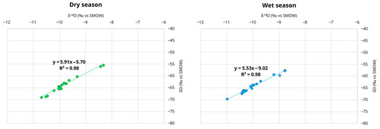
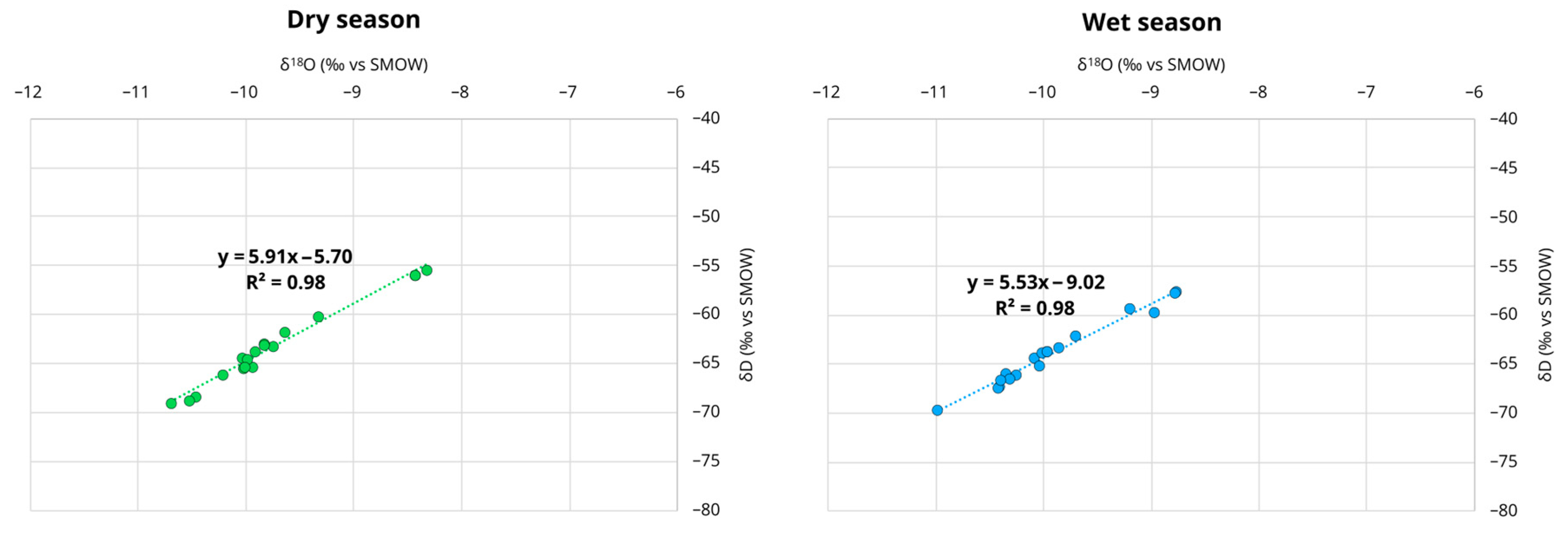
The δ¹⁸O–δD relationships (Figure 5) show excellent linear fit, defined by

δD = (5.91 ± 0.85) δ¹⁸O − (5.70 ± 0.01)

(3)

for the dry season, and

δD = (5.53 ± 0.97) δ¹⁸O − (9.02 ± 0.02)

(4)

for the wet season, both with coefficients of determination R² = 0.98.

Mean isotopic infiltration altitude was estimated for each of the three groundwater bodies using locally constrained δ¹⁸O–elevation correlation lines. The following relationships were applied

h (m a.s.l.) = −769 δ¹⁸O − 6460

(5)

for the Genzana–Greco Mts. aquifer [7],

h (m a.s.l.) = −835 δ¹⁸O − 7500

(6)

for the Morrone Mt. aquifer [8], and

h (m a.s.l.) = −526 δ¹⁸O − 3595

(7)

for the Marsicano Mt. aquifer [9].

3.2. Genzana–Greco Mts. Aquifer

As can be seen in

Table 3. Mean isotopic infiltration altitude (MIIA) estimated for Genzana–Greco Mts.’ springs using Equation (5). See Figure 2 for location.

Spring	Label	MIIA Dry Season (m a.s.l.)	MIIA Wet Season (m a.s.l.)	Spring Altitude (m a.s.l.)
Capolaia	G-G1_a	1590	1550	685
Germina	G-G1_b	1640	1560	650
Acquachiara	G-G5	1190	1260	310

, the estimated mean isotopic infiltration altitude values for the Germina and Capolaia springs are nearly coincident and exhibit seasonal variations following the same trend. Both observations support recharge from a single sector of the groundwater body, as further supported by the electrical conductivity and temperature steady data reported in the spring datasets (Table 2).

The mean isotopic infiltration altitude estimated for the Acquachiara spring allows the exclusive recharge from the alluvial deposits of the Sulmona plain and from the Introdacqua alluvial fan (Figure 2B) to be unequivocally excluded, as these are located at elevations significantly lower than those indicated by the isotopic results. However, the available data do not allow differentiation between a potential recharge from the Genzana–Greco aquifer and from the adjacent aquifer, whose mean isotopic elevations are comparable.

Regarding the origin of the Acquachiara spring [41], based on discharge measurements along the Gizio River upstream of the spring area and at the spring itself, assumed a predominant recharge from the carbonate Genzana–Greco aquifer, overlain by a shallower circulation component fed by the Introdacqua alluvial fan and the Gizio River (Figure 2).

In the absence of more detailed investigations, the recharge of the Acquachiara spring cannot be attributed with absolute certainty exclusively to the Genzana–Greco aquifer.

Moreover, the wet and dry seasons’ altitudes give more information about the Genzana–Greco aquifer: the slight differences in the seasonal MIIA suggest that the aquifer is sufficiently wide to not be affected by periodic variations. This behavior is supported by the constancy of electric conductivity and temperature values throughout the seasons (Table 2).

Considering the limitations discussed in Section 2.2.2, which preclude absolute interpretations and allow only relative assessments, a contribution of more recent surface waters can be observed during the wet season in the Capolaia and Acquachiara springs as the MRT decreases visibly in the wet season. This finding is consistent with the fact that both springs receive inputs from alluvial deposits, at least in proximity to their points of emergence (

Table 4. Mean Residence Time (MRT) for water samples from Genzana–Greco Mts.’ springs using Equation (2). See Figure 2 for location.

Spring Name	Label	MRT (y) (TU 4.5)	MRT (y) (TU 8.5)	Tritium Dosage (TU)
Capolaia	G-G1_a (ds)	8.3	19.7	2.8
	G-G1_a (ws)	5.0	16.4	3.4
Germina	G-G1_b (ds)	1.7	13.1	4.1
	G-G1_b (ws)	6.6	18.0	3.1
Acquachiara	G-G5 (ds)	12.3	23.8	2.3
	G-G5 (ws)	3.2	14.6	3.8

ds: dry season; ws: wet season.

).

The results obtained for the Germina spring should be considered preliminary and warrant further monitoring.

3.3. Morrone Mt. Aquifer

As can be seen in

Table 5. Mean isotopic infiltration altitude (MIIA) estimated for Morrone Mt.’s springs using Equation (6). See Figure 3 for location.

Spring	Label	MIIA Dry Season (m a.s.l.)	MIIA Wet Season (m a.s.l.)	Spring Altitude (m a.s.l.)
Giardino	MR1_a	1420	1660	250
Pescara river	MR4_a; b_I	830	1130	230–215
	MR4_a; b_II	850	1050	230–215
	MR4_a; b_III	850	1100	230–215
	MR4_a; b_IV	1020	1170	230–215

, the MIIAs of the wet season are higher than those of the dry season, which indicates a seasonal variation in the aquifer recharge, these higher values during the wet season can also be evidence of the contribution of snowmelt. The aquifers investigated clearly belong to systems whose recharge is partly driven by snowmelt [42,43].

The results obtained for the spring pools located within the Pescara River channel (Figure 3) indicate a mean isotopic infiltration altitude consistent with the mean elevations of the northern sector of the Morrone massif, which reach maximum elevations of approximately 1700 m a.s.l. These values allow local meteoric recharge to be excluded, as it would be expected to occur at significantly lower elevations. Moreover, since the spring pools are located several meters above the riverbed, a direct contribution from river water can also be ruled out.

The results gained for the Giardino spring allow the recharge feeding this spring to be attributed to the central–southern sectors of the aquifer, where the massif elevations reach about 2000 m a.s.l.

Overall, these results confirm the hydrogeological model that identifies the discharge gains within the Pescara River channel as one of the two main basal outlets of the aquifer.

Considering the limitations discussed in Section 2.2.2, which allow only relative interpretation of the data, the MRT values (

Table 6. Mean Residence Time (MRT) estimation for water samples from Morrone Mt.’s springs using Equation (2). See Figure 3 for location.

Spring Name	Label	MRT (y) (TU 4.5)	MRT (y) (TU 8.5)	Tritium Dosage (TU)
Giardino	MR1_a (ds)	12.4	23.8	2.3
	MR1_a (ws)	8.1	19.5	2.9
Pescara river	MR4_a; b_I (ds)	8.9	20.3	2.7
	MR4_a; b_I (ws)	15.5	26.9	1.9
	MR4_a; b_II (ds)	5.9	17.3	3.2
	MR4_a; b_II (ws)	7.7	19.1	2.9
	MR4_a; b_III (ds)	11.6	23.0	2.4
	MR4_a; b_III (ws)	8.8	20.2	2.8
	MR4_a; b_IV (ds)	12.8	24.2	2.2
	MR4_a; b_IV (ws)	11.2	22.6	2.4

ds: dry season; ws: wet season.

) of the Pescara River channel gains within the Gole di Popoli are comparable to those of the Giardino spring. This finding further supports the interpretation that these gains originate from the basal aquifer of the Morrone massif. Only one of the in-channel spring (MR4a; b_II) shows evidence of a probable contribution from faster flow paths, likely related to interaction with Pescara River waters.

3.4. Marsicano Mt. Aquifer

The δ¹⁸O and δD isotopic analyses, processed and interpreted according to the methodology described in Section 2.2.1, yielded the results reported in

Table 7. Mean isotopic infiltration altitude (MIIA) estimated for Marsicano Mt.’s springs using Equation (7). See Figure 4 for location.

Spring	Label	MIIA Dry Season (m a.s.l.)	MIIA Wet Season (m a.s.l.)	Spring Altitude (m a.s.l.)
La Marca	MS1_a	1320	1250	950
Villalago	MS4_a_I	850	1130	900
	MS4_a_II	850	1020	900–800
	MS4_a_III	1480	1510	900–800
	MS4_a_IV	800	1030	900–800
Sega	MS4_b	1690	1720	800
Cavuto	MS5_c	1540	1600	500
	MS5_a_I	1590	1650	515
	MS5_a_II	1590	1680	515
	MS5_a_III	1630	1650	515

; these allow researchers to confirm the hydrogeological model of the Marsicano Mt. aquifer (Figure 4) and to define the discharge monitoring points.

The estimation of mean isotopic infiltration altitude values confirms the findings of Petitta et al. [9] regarding the role of Lake Scanno and the landslide deposits from which it originated. The Villalago springs exhibit mean isotopic infiltration altitude values lower than the average of the aquifer and consistent with the elevation of the lake, or only slightly higher (approximately 800–1100 m a.s.l.). These springs show high variations in seasonal MIIA values, confirming the Lake Scanno influence and, like Morrone Mt. ones, a snowmelt possible contribution during the wet season.

Exceptions are represented by the MS4_a_III spring, whose mean isotopic infiltration altitude, already highlighted in [9], is approximately 1500 m a.s.l., and by the Sega spring, which shows a mean isotopic infiltration altitude of about 1700 m a.s.l., both values are consistent with the highest mean elevations of the Marsicano Mt.

These results are supported by electrical conductivity and temperature data (Table 2), which show lower values than those measured at the Villalago springs, with slight seasonal variability.

Isotopic analyses allow the increase in discharge of the Sagittario River downstream of the Cavuto group (MS5_c in Figure 4A) to be attributed to the same groundwater system feeding the Cavuto springs, with a mean isotopic infiltration altitude of approximately 1600 m a.s.l.

The mean isotopic infiltration altitude estimates for the Cavuto group also suggest that the recharge areas cannot be attributed exclusively to the northern sector of the Marsicano massif [30] but instead receive contributions from higher and more central portions of the system.

Table 8. Mean Residence Time (MRT) estimation for water samples from Marsicano Mt.’s springs using Equation (2). See Figure 4 for location.

Spring Name	Label	MRT (y) (TU 4.5)	MRT (y) (TU 8.5)	Tritium Dosage (TU)
La Marca	MS1_a (ds)	5.0	16.4	3.4
	MS1_a (ws)	1.0	12.4	4.3
Villalago gr.	MS4_a_I (ds)	9.8	21.2	2.6
	MS4_a_I (ws)	0.9	12.3	4.3
	MS4_a_II (ds)	7.9	19.3	2.9
	MS4_a_II (ws)	8.6	20.0	2.8
	MS4_a_III (ds)	10.5	22.0	2.5
	MS4_a_III (ws)	11.7	23.1	2.3
	MS4_a_IV (ds)	7.3	18.7	3.0
	MS4_a_IV (ws)	6.7	18.1	3.1
Sega	MS4_b (ds)	10.5	22.0	2.5
	MS4_b (ws)	12.4	23.8	2.3
Cavuto	MS5_c (ds)	8.5	19.9	2.8
	MS5_c (ws)	5.0	16.4	3.4
	MS5_a_I (ds)	6.1	17.5	3.2
	MS5_a_I (ws)	11.2	22.6	2.4
	MS5_a_II (ds)	7.3	18.7	3.0
	MS5_a_II (ws) MS5_a_III (ds)	8.9	20.3	2.7
		16.0	27.4	1.8
	MS5_a_III (ws)	8.7	20.1	2.8

ds: dry season; ws: wet season.

shows the tritium analyses results, which must be considered taking into account the limitations discussed in Section 2.2.2; these allow only relative interpretations, the MS4_a_III spring and the Sega spring, besides being recharged from higher isotopic elevations than the rest of the group, are also characterized by slower flow circuits. In contrast, other springs, such as La Marca and the MS4_a_I spring (located along the Sagittario River channel), appear to be influenced by direct precipitation inputs, as indicated by low MTR values during the high-flow season.

For the Cavuto group, tritium analyses indicate seasonally variable transit times. This behavior is likely related to the proximity of the Sagittario stream and its role in recharging the spring.

4. Conclusions

From a general methodological perspective, all results indicate mean isotopic infiltration altitudes (MIIAs) consistent with the morphology of the aquifers. High-flow basal springs show minimal MIIA variations of 20–80 m, with the highest values occurring during the wet season. Larger variations, on the order of 250–300 m, are observed in springs where recharge is influenced by surface water or snowmelt contributions.

At the level of individual aquifers, although not conclusively, MIIA estimations and the seasonal variations in δ¹⁸O–δD helped refine the understanding of the basal spring recharge circuits in the Genzana–Greco Mts., Morrone Mt., and Marsicano Mt. aquifers.

In the Genzana–Greco aquifer, results indicate that the Germina and Capolaia springs share a common recharge sector, while the Acquachiara spring is mainly fed by higher-elevation carbonate areas, excluding significant contributions from local alluvial deposits. For the Morrone aquifer, isotopic and tritium data confirm recharge from the central–southern massif and support the identification of basal springs and Pescara River gains as primary discharge points, with minimal influence from surface water. In the Marsicano aquifer, the analyses highlight Lake Scanno’s role in the recharge of Villalago springs and delineate the Cavuto group as a major discharge system receiving inputs from central and northern sectors of the massif.

Overall, the combination of δ¹⁸O–δD and tritium measurements proved essential in constraining recharge elevations, flow dynamics, and seasonal variations, particularly in regions where morphological boundaries do not correspond to hydrogeological ones.

These findings provide a more robust framework for groundwater management, supporting sustainable exploitation, protection of drinking water resources, and informed planning for the monitoring of karst and alluvial aquifers in the central Apennines and similar geological, geomorphological, and hydrogeological frameworks.

Tritium-based Mean Residence Time (MRT) estimates yielded tentative results that are only qualitatively reliable and not quantitatively robust. This is due to the limited constraint on atmospheric tritium concentrations, particularly at the time of infiltration, and to the intrinsic approximations of the analytical methods.

References

- Celico, P. Schema Idrogeologico Dell’Appennino Carbonatico Centro-Meridionale. Mem. Note Dell’istituto Geol. Appl. Dell’università Napoli 1979, 14, 5–97. [Google Scholar]
- Cassa per il Mezzogiorno; Celico, P. Idrogeologia Dell’Italia Centro-Meridionale. Progetti Speciali per Gli Schemi Idrici Nel Mezzogiorno. Quad. Cassa Mezzog. 1983, 4.2. Available online: https://aset.acs.beniculturali.it/aset-web/biblio/detail/IT-ACS-BIB00001-0000074/quaderno-4-2-progetti-speciali-schemi-idrici-nel-mezzogiorno-idrogeologia-italia-centro-meridionale.html?currentNumber=10 (accessed on 7 April 2026).
- Boni, C.; Bono, P.; Capelli, G. Schema Idrogeologico Dell’Italia Centrale. Mem. Della Soc. Geol. Ital. 1986, 35, 991–1012. [Google Scholar]
- Fiorillo, F.; Petitta, M.; Preziosi, E.; Rusi, S.; Esposito, L.; Tallini, M. Long-Term Trend and Fluctuations of Karst Spring Discharge in a Mediterranean Area (Central-Southern Italy). Environ. Earth Sci. 2015, 74, 153–172. [Google Scholar] [CrossRef] [Scilit]
- Medici, G.; Lorenzi, V.; Sbarbati, C.; Manetta, M.; Petitta, M. Structural Classification, Discharge Statistics, and Recession Analysis from the Springs of the Gran Sasso (Italy) Carbonate Aquifer; Comparison with Selected Analogues Worldwide. Sustainability 2023, 15, 10125. [Google Scholar] [CrossRef] [Scilit]
- Giacopetti, M.; Materazzi, M.; Pambianchi, G.; Posavec, K. Analysis of Mountain Springs Discharge Time Series in the Tennacola Stream Catchment (Central Apennine, Italy). Environ. Earth Sci. 2016, 76, 20. [Google Scholar] [CrossRef] [Scilit]
- Barbieri, M.; D’Amelio, L.; Desiderio, G.; Marchetti, A.; Nanni, T.; Petitta, M.; Rusi, S.; Tallini, M. Gli Isotopi Ambientali (18O, 2H e 87Sr/86Sr) Nelle Acque Sorgive Dell’Appennino Abruzzese: Considerazioni Sui Circuiti Sotterranei Negli Acquiferi Carbonatici. 2003. ISBN 8886698402. Available online: https://www.researchgate.net/publication/265972148_Gli_isotopi_ambientali_18O_2H_e_87Sr86Sr_nelle_acque_sorgive_dell%27Appennino_abruzzese_considerazioni_sui_circuiti_sotterranei_negli_acquiferi_carbonatici (accessed on 7 April 2026).
- Desiderio, G.; Ferracuti, L.; Rusi, S.; Tatangelo, F. Il Contributo Degli Isotopi Naturali 18O e 2H Nello Studio Delle Idrostrutture Carbonatiche Abruzzesi e Delle Acque Mineralizzate Nell’area Abruzzese e Molisana. G. Geol. Appl. 2005, 2, 453–458. [Google Scholar]
- Petitta, M.; Scarascia Mugnozza, G.; Barbieri, M.; Bianchi Fasani, G.; Esposito, C. Hydrodynamic and Isotopic Investigations for Evaluating the Mechanisms and Amount of Groundwater Seepage through a Rockslide Dam. Hydrol. Process. 2010, 24, 3510–3520. [Google Scholar] [CrossRef] [Scilit]
- Tallini, M.; Adinolfi Falcone, R.; Carucci, V.; Falgiani, A.; Parisse, B.; Petitta, M. Isotope Hydrology and Geochemical Modeling: New Insights into the Recharge Processes and Water–Rock Interactions of a Fissured Carbonate Aquifer (Gran Sasso, Central Italy). Environ. Earth Sci. 2014, 72, 4957–4971. [Google Scholar] [CrossRef] [Scilit]
- Kattan, Z. Environmental Isotope Study of the Major Karst Springs in Damascus Limestone Aquifer Systems: Case of the Figeh and Barada Springs. J. Hydrol. 1997, 193, 161–182. [Google Scholar] [CrossRef] [Scilit]
- Kattan, Z. Use of Hydrochemistry and Environmental Isotopes for Evaluation of Groundwater in the Paleogene Limestone Aquifer of the Ras Al-Ain Area (Syrian Jezireh). Environ. Geol. 2001, 41, 128–144. [Google Scholar] [CrossRef] [Scilit]
- Marfia, A.M.; Krishnamurthy, R.V.; Atekwana, E.A.; Panton, W.F. Isotopic and Geochemical Evolution of Ground and Surface Waters in a Karst Dominated Geological Setting: A Case Study from Belize, Central America. Appl. Geochem. 2004, 19, 937–946. [Google Scholar] [CrossRef] [Scilit]
- Jiménez-Madrid, A.; Castaño, S.; Vadillo, I.; Martinez, C.; Carrasco, F.; Soler, A. Applications of Hydro-Chemical and Isotopic Tools to Improve Definitions of Groundwater Catchment Zones in a Karstic Aquifer: A Case Study. Water 2017, 9, 595. [Google Scholar] [CrossRef] [Scilit]
- Jódar, J.; Herms, I.; Lambán, L.J.; Martos-Rosillo, S.; Herrera-Lameli, C.; Urrutia, J.; Soler, A.; Custodio, E. Isotopic Content in High Mountain Karst Aquifers as a Proxy for Climate Change Impact in Mediterranean Zones: The Port Del Comte Karst Aquifer (SE Pyrenees, Catalonia, Spain). Sci. Total Environ. 2021, 790, 148036. [Google Scholar] [CrossRef] [Scilit]
- Iacurto, S.; Grelle, G.; De Filippi, F.M.; Sappa, G. Karst Recharge Areas Identified by Combined Application of Isotopes and Hydrogeological Budget. Water 2021, 13, 1965. [Google Scholar] [CrossRef] [Scilit]
- Rusjan, S.; Sapač, K.; Petrič, M.; Lojen, S.; Bezak, N. Identifying the Hydrological Behavior of a Complex Karst System Using Stable Isotopes. J. Hydrol. 2019, 577, 123956. [Google Scholar] [CrossRef] [Scilit]
- Lorenzi, V.; Barberio, M.D.; Sbarbati, C.; Petitta, M. Groundwater Recharge Distribution Due to Snow Cover in Shortage Conditions (2019–22) on the Gran Sasso Carbonate Aquifer (Central Italy). Environ. Earth Sci. 2023, 82, 206. [Google Scholar] [CrossRef] [Scilit]
- Barbieri, M.; Boschetti, T.; Petitta, M.; Tallini, M. Stable Isotope (2H, 18O and 87Sr/86Sr) and Hydrochemistry Monitoring for Groundwater Hydrodynamics Analysis in a Karst Aquifer (Gran Sasso, Central Italy). Appl. Geochem. 2005, 20, 2063–2081. [Google Scholar] [CrossRef] [Scilit]
- Sappa, G.; Vitale, S.; Ferranti, F. Identifying Karst Aquifer Recharge Areas Using Environmental Isotopes: A Case Study in Central Italy. Geosciences 2018, 8, 351. [Google Scholar] [CrossRef] [Scilit]
- Petitta, M.; Banzato, F.; Lorenzi, V.; Matani, E.; Sbarbati, C. Determining Recharge Distribution in Fractured Carbonate Aquifers in Central Italy Using Environmental Isotopes: Snowpack Cover as an Indicator for Future Availability of Groundwater Resources. Hydrogeol. J. 2022, 30, 1619–1636. [Google Scholar] [CrossRef] [Scilit]
- Nanni, T.; Desiderio, G.; Fochi Vici, C.; Petitta, M.; Ruggieri, G.; Rusi, S.; Tallini, M.; Vivalda, P.M. Schema Idrogeologico Dell’Italia Centro-Adriatica. Scala 1:250.000. 2011. Available online: https://iris.univpm.it/handle/11566/66615 (accessed on 7 April 2026).
- Desiderio, G.; D’arcevia, C.F.V.; Nanni, T.; Rusi, S. Hydrogeological Mapping of the Highly Anthropogenically Influenced Peligna Valley Intramontane Basin (Central Italy). J. Maps 2012, 8, 165–168. [Google Scholar] [CrossRef] [Scilit]
- Conese, M.; Nanni, T.; Peila, C.; Rusi, S.; Salvati, R. Idrogeologia Della Montagna Del Morrone (Appennino Abruzzese): Dati Preliminari. Mem. Della Soc. Geol. 2001, 56, 181–196. [Google Scholar]
- Massoli-Novelli, R.; Petitta, M.; Salvati, R. La Situazione Idrogeologica e Ambientale Delle Gole Di Popoli (Abruzzo): Primi Risultati e Prospettive Della Ricerca. Mem. Della Soc. Geol. 1998, 53, 563–584. [Google Scholar]
- Regione Abruzzo; Settore Lavori Pubblici e Politica della Casa; Servizio Difesa e Tutela del Suolo. Aquater Studi Geomorfologici, Idrogeologici e Delle Risorse Idriche Del Territorio Regionale—Geomorfologia, Relazione e Schede, internal report. 1993.
- Regione Abruzzo Piano Di Tutela Delle Acque (PTA)—Relazione Idrogeologica (Elab. A1.2). 2008. Available online: https://www2.regione.abruzzo.it/system/files/urbanistica-territorio/piano-tutela-acque/prop-gr-appr-finale/All_A1_2/RELAZIONE_IDROGEOLOGICA.pdf (accessed on 7 April 2026).
- Di Curzio, D.; Rusi, S.; Semeraro, R. Multi-Scenario Numerical Modeling Applied to Groundwater Contamination: The Popoli Gorges Complex Aquifer Case Study (Central Italy). Acque Sotter. Ital. J. Groundw. 2018, 7, 49–58. [Google Scholar] [CrossRef] [Scilit]
- Boni, C.; Bono, P.; Capelli, G. Schema Idrogeologico Dell’Italia Centrale—Sheet A. Memorie della Società Geologica Italiana. 1986. Available online: https://www.idrogeologiaquantitativa.it/wordpress/wp-content/uploads/2009/11/Cart_1986_CartaIdroItaliaCentrale_A.pdf (accessed on 7 April 2026).
- Boni, C.; Ruisi, M. Carta Idrogeologica Della Marsica Orientale (M. Marsicano—M.Gna Grande) Scala 1:50.000; GNDCI-CNR: Rome, Italy, 2005. [Google Scholar]
- Longinelli, A.; Selmo, E. Isotopic Composition of Precipitation in Italy: A First Overall Map. J. Hydrol. 2003, 270, 75–88. [Google Scholar] [CrossRef] [Scilit]
- Eyrolle, F.; Ducros, L.; Le Dizès, S.; Beaugelin-Seiller, K.; Charmasson, S.; Boyer, P.; Cossonnet, C. An Updated Review on Tritium in the Environment. J. Environ. Radioact. 2018, 181, 128–137. [Google Scholar] [CrossRef] [Scilit] [PubMed]
- Civita, M. Idrogeologia Applicata e Ambientale; Casa Editrice Ambrosiana: Milan, Italy, 2005. [Google Scholar]
- Fornaseri, M. Lezioni Di Geochimica; CEA: Milan, Italy, 1988. [Google Scholar]
- Juhlke, T.R.; Sültenfuß, J.; Trachte, K.; Huneau, F.; Garel, E.; Santoni, S.; Barth, J.A.C.; van Geldern, R. Tritium as a Hydrological Tracer in Mediterranean Precipitation Events. Atmos. Chem. Phys. 2020, 20, 3555–3568. [Google Scholar] [CrossRef] [Scilit]
- Longinelli, A.; Deganello, S. Introduzione Alla Geochimica. UTET Torino; UTET: Turin, Italy, 1999. [Google Scholar]
- IAEA (International Atomic Energy Agency). WISER (Water Isotope System for Data Analysis) Visualization and Electronic Retrieval. Available online: https://Nucleus.Iaea.Org/Wiser/Index.Aspx (accessed on 7 April 2026).
- Bono, P.; Gonfiantini, R.; Alessio, M.; Fiori, C.; D’Amelio, L. Stable Isotopes (δ18O, δ2H) and Tritium in Precipitation: Results and Comparison with Groundwater Perched Aquifers in Central Italy In, Isotopic Composition of Precipitation in the Mediterranean Basin in Relation to Air Circulation Patterns and Climate. Final Report of a Coordinated Research Project 2000–2004. 2005. Available online: https://www-pub.iaea.org/MTCD/Publications/PDF/te_1453_web.pdf (accessed on 7 April 2026).
- Tazioli, A. Landfill Investigation Using Tritium and Isotopes as Pollution Tracers. Aqua Mundi 2011, 1, 83–91. [Google Scholar]
- Gröning, M.; Rozanski, K. Uncertainty Assessment of Environmental Tritium Measurements in Water. Accredit. Qual. Assur. 2003, 8, 359–366. [Google Scholar] [CrossRef] [Scilit]
- Desiderio, G.; Nanni, T.; Rusi, S. Idrogeologia e qualità delle acque degli acquiferi della conca intramontana di Sulmona (Abruzzo). In Proceedings of the AIGA–I Congresso Nazionale, Atti, Chieti, Italy, 19–20 February 2003; Available online: https://www.researchgate.net/publication/265972179_Idrogeologia_e_qualita_delle_acque_degli_acquiferi_della_conca_intramontana_di_Sulmona_Abruzzo (accessed on 7 April 2026).
- Chiaudani, A.; Di Curzio, D.; Rusi, S. The Snow and Rainfall Impact on the Verde Spring Behavior: A Statistical Approach on Hydrodynamic and Hydrochemical Daily Time-Series. Sci. Total Environ. 2019, 689, 481–493. [Google Scholar] [CrossRef] [Scilit] [PubMed]
- Rusi, S.; Di Giovanni, A. Assessing the Impact of Often Overlooked Snowfall on the Hydrological Balance of Apennine Mountain Aquifers in Central Italy. Water 2025, 17, 864. [Google Scholar] [CrossRef] [Scilit]
Disclaimer/Publisher’s Note: The statements, opinions and data contained in all publications are solely those of the individual author(s) and contributor(s) and not of MDPI and/or the editor(s). MDPI and/or the editor(s) disclaim responsibility for any injury to people or property resulting from any ideas, methods, instructions or products referred to in the content. |
© 2026 by the authors. Licensee MDPI, Basel, Switzerland. This article is an open access article distributed under the terms and conditions of the Creative Commons Attribution (CC BY) license.