Exploring the Seven Climate Zones of China: How Soil Moisture and Vapor Pressure Deficit Influence Vegetation Productivity

Abstract

Reduced soil moisture (SM) together with elevated vapor pressure deficit (VPD) suppresses gross primary productivity (GPP) and thus weakens the capacity of the terrestrial carbon pool. Against the backdrop of global climate change, soil and atmospheric drought exert a more profound impact on vegetation growth, and their combined impacts remain unclear. Based on multi-source remote sensing observations and reanalysis datasets, three vegetation remote sensing indices, GPP, SIF, and NDVI (collectively referred to as Vegetation Remote Sensing Indices, VSI), are employed in this study to assess the relative impacts of soil and atmospheric drought on terrestrial vegetation. First, Copula-based conditional probabilities are applied to identify which factor (reduced SM or high VPD) plays a dominant role under conditions of declining vegetation productivity and to determine their corresponding thresholds. Furthermore, the underlying driving mechanisms are elucidated by utilizing Structural Equation Modeling (SEM) for path analysis to clarify how climatic factors indirectly affect vegetation productivity by influencing SM and VPD. The results suggest that vegetation growth in China’s different climatic zones is affected by distinct factors. Specifically, SM is the primary factor influencing vegetation productivity, dominating 71.16% of the nation’s vegetated areas. Its influence is particularly pronounced in arid and semi-arid regions. In contrast, the impact of VPD is predominantly concentrated in semi-humid plain regions. Furthermore, the critical thresholds for SM in different climate zones are identified: the threshold averages approximately 0.33 m³/m³ in humid and plateau regions and 0.13 m³/m³ in arid and semi-arid regions. The SEM analysis further reveals the complex pathways by which climatic variables influence vegetation growth. In SM-dominated regions, higher SM directly promotes vegetation growth; in VPD-dominated regions, drier air imposes a stronger suppression on vegetation growth. Nonetheless, the plateau temperate semi-arid zone demonstrates distinct hydrometeorological characteristics. Attributed to the region’s unique hydrometeorological conditions, the negative effects of higher VPD are generally outweighed by the favorable conditions for photosynthesis with which it co-occurs. These findings clarify the intricate impacts of SM and VPD on vegetation productivity, providing a foundational framework for the development of tailored ecological management strategies and drought early warning systems.

1. Introduction

Terrestrial vegetation productivity, as the largest carbon flux within the global carbon budget, critically assists in sustaining the carbon balance of terrestrial ecosystems, yet it remains highly sensitive to changes in moisture conditions [1]. Drought, a recurrent and severe manifestation of abiotic stress, significantly suppresses vegetation productivity [2]. Plant growth is primarily regulated by two distinct types of droughts: soil drought, characterized by reduced SM; atmospheric drought, expressed as an elevated VPD within the soil-plant-atmosphere continuum (SPAC) [3,4]. They jointly influence vegetation function. As SM and VPD critically impact plant physiological processes, disentangling their crucial roles in the decline of GPP helps reveal the driving mechanisms of ecological drought and more effectively simulate drought processes in Earth System Models [5].

Additionally, SM and VPD are the vital factors constraining vegetation productivity at the global scale [6]. Nevertheless, such global-scale studies typically fail to fully account for regional climatic heterogeneity, particularly in geographically complex regions like China [7]. China possesses a vast territory featuring a unique three-tiered topographic structure and significant monsoon influence, bringing about highly distinct climatic zones ranging from arid inland basins to humid coastal regions. Consequently, limited knowledge exists with regard to the relatively dominant roles of the two factors in vegetation stress and their potential threshold effects. Previous research has largely focused on single-threshold analyses of either soil or atmospheric drought, or has been restricted to meteorological drought indices of the Standardized Precipitation Evapotranspiration Index (SPEI). Nonetheless, there is little research on the threshold effects of both SM and VPD. Thus, a consensus remains elusive regarding the crucial roles of SM and VPD across varying spatial scales, which further necessitates the conduction of regional-scale research.

However, linear modeling approaches are predominantly employed in most existing studies [8,9] to examine how SM and VPD impact GPP. This limits their ability to represent the intrinsic non-linear coupling between these factors. Compared with traditional linear methods, Copula models can flexibly describe non-linear and asymmetric dependencies between variables and accurately capture joint extremes, enabling them to identify compound drought events. Consequently, the mechanisms of their compound effects, particularly under extreme conditions, remain unclear. While recent research has begun to address extreme events, the triggering mechanisms of compound extremes driven by the interaction of SM and VPD have not been thoroughly investigated. Furthermore, the common binning analyses and regression methods are ill-suited to directly quantify the risk of GPP decline [10,11,12]. Hence, identifying the relative contributions of SM and VPD to GPP decline and revealing their complex mechanisms under China’s diverse climatic conditions hold substantial scientific significance. This study aims to overcome the limitations of traditional linear frameworks. Specifically, two-dimensional (2D) and three-dimensional (3D) Copula methods [13,14] are innovatively employed to systematically elucidate the non-linear impacts of the two factors on GPP and the formation mechanisms of their compound extreme events.

Currently, indicators such as the three vegetation remote sensing indices GPP, Solar-Induced Chlorophyll Fluorescence (SIF), and the Normalized Difference Vegetation Index (NDVI) are commonly applied to evaluate vegetation productivity, whereas each metric has its own applicability and limitations [15]. For example, GPP fails to account for autotrophic respiration, making it difficult to accurately reflect net carbon sink capacity [16]. While SIF is highly sensitive to photosynthetic dynamics, its signal is susceptible to interference from various factors, introducing significant uncertainties in its interpretation [17]. In addition, the widely applied NDVI tends to experience signal saturation in areas characterized by dense vegetation cover [18]. Existing research predominantly relies on single data sources while generally lacking synergistic comparison and comprehensive validation across multi-source data. Consequently, it remains challenging to delineate the commonalities and discrepancies among these different metrics regarding their response mechanisms and representational capabilities. Therefore, in this study, multi-source datasets (GPP, SIF, and NDVI) are integrated, and a rigorous cross-validation against three major reanalysis datasets (ERA5-Land, GLDAS, and CRU) [19,20] is conducted to elucidate the response patterns of vegetation dynamics from a multi-metric synergistic perspective. The results demonstrate the improved comprehensiveness and reliability of understanding ecosystem carbon cycle processes.

Furthermore, significant progress has been made in elucidating the relationship between climatic factors and vegetation productivity [6,7]. Nevertheless, most studies remain limited to analyzing the direct effects of single variables (such as SM or VPD) and commonly fail to integrate multiple factors and delineate their complex interaction pathways. Currently, few studies simultaneously incorporate total precipitation (TP), SM, VPD, surface net solar radiation (SSR), temperature (TM), relative humidity (RH), and vegetation productivity metrics (such as GPP, SIF, and NDVI) within a unified analytical framework. Consequently, it is difficult to systematically resolve the direct and indirect causal linkages among these factors across different climatic zones. The lack of an integrated approach impedes a deeper understanding of the regional disparities and mechanistic complexities governing vegetation responses under changing climatic conditions. Therefore, a comprehensive Structural Equation Model (SEM) [21] is developed in this study to systematically elucidate the synergistic effects of the aforementioned multi-factors on vegetation productivity across different climatic zones in China. Specifically, the core scientific hypothesis of this study is that the dominant driver of vegetation productivity decline, that is, whether SM deficit or atmospheric aridity (VPD), diverges spatially across China’s heterogeneous climatic zones, and that compound extremes amplify these risks through distinct non-linear mechanisms and thresholds compared to single-factor stressors.

First, bivariate Copula models are constructed for “SM–Vegetation Productivity (GPP, NDVI, SIF)” and “VPD–Vegetation Productivity (GPP, NDVI, SIF),” respectively. The differential sensitivities of various regions to SM and VPD stress are preliminarily identified by quantifying the conditional probability of a significant productivity decline under single-factor stress. Building on this, a trivariate Copula model (SM-VPD-Vegetation Productivity) is designed to precisely quantify the joint probability of productivity decline under the “low SM–high VPD” compound stress scenario. The spatial distribution patterns of SM- and VPD-dominated regions are identified by integrating these results with the single-factor conditional probabilities derived from the bivariate models. Subsequently, within the delineated dominant areas, an iterative threshold method is employed following Copula conditional probabilities. The critical SM and VPD thresholds that trigger vegetation productivity decline in each region are determined by iteratively calculating the SM and VPD values related to the conditional probability first reaching 50%. This lays a quantitative foundation for stress early warning systems. Finally, the linear associations are verified by calculating Pearson correlation coefficients between productivity and SM/VPD. Afterward, crucial climatic factors (such as TM and TP) are incorporated by a SEM to systematically reveal the direct effects of SM and VPD on productivity, as well as the indirect transmission mechanisms via the “Climatic factors→SM/VPD→Productivity” pathways. This approach allows for a thorough understanding of the underlying mechanisms through which SM-VPD stress affects vegetation productivity.

2. Materials and Methods

2.1. Study Area

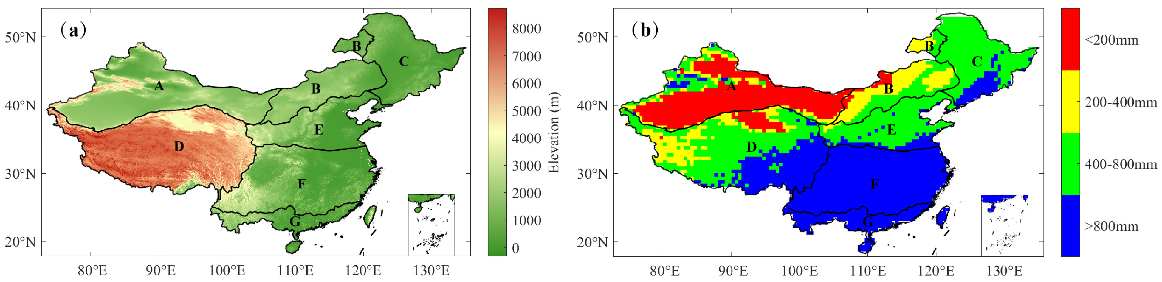
China possesses a vast territory and complex topography, featuring a three-tiered ‘ladder’ structure that descends in altitude from west to east (Figure 1a). The western region, forming the first tier, is dominated by the Tibetan Plateau, with an average elevation of >4000 m; the central region forms the second tier, consisting of the Inner Mongolia Plateau, the Loess Plateau, and the Yunnan-Guizhou Plateau, with an elevation in the range of 1000–2000 m; the eastern region constitutes the third tier, characterized by widespread plains, low mountains, and hills [22]. This complex topographical pattern profoundly influences the climate and precipitation distribution across China.

The study area encompasses seven major climatic zones: (A) mid-temperate arid, (B) mid-temperate semi-arid, (C) mid-temperate semi-humid, (D) plateau temperate semi-arid, (E) warm-temperate semi-humid, (F) north subtropical humid, and (G) marginal tropical humid [23]. According to precipitation data (2000–2020), China’s precipitation exhibits highly significant spatial differentiation (Figure 1b). Specifically, precipitation declines from the southeastern coastal areas to the northwest inland, and annual rainfall sharply drops from over 800 mm to less than 200 mm. Meanwhile, the annual precipitation in the transitional zones (B, C, and E) ranges between 200 and 800 mm [19,23]. This spatial heterogeneity in climate and precipitation is of critical importance to the region’s ecosystems and agricultural production.

2.2. Datasets

Multiple datasets were integrated for vegetation productivity, SM, VPD, and other climate variables to examine the impacts of soil and atmospheric drought on China’s terrestrial ecosystem productivity.

Table 1. Summary of datasets used in this study.

Variable Type	Dataset Name	Original Temporal Coverage	Temporal Coverage Used in Study
Vegetation Productivity	NIRv GPP	2000–2018	2000–2018
	MOD13A3 NDVI	2000–2023	2000–2020
	GOSIF_v2	2000–2023	2000–2020
SM	ERA5-Land	2000–2020	2000–2018 (for GPP groups) & 2000–2020 (for NDVI/SIF groups)
	GLDAS Noah V2.1	2000–2020	2000–2018 (for GPP groups) & 2000–2020 (for NDVI/SIF groups)
	GLEAM v4.2a	2000–2020	2000–2018 (for GPP groups) & 2000–2020 (for NDVI/SIF groups)
VPD & Climate	ERA5-Land	2000–2020	2000–2018 (for GPP groups) & 2000–2020 (for NDVI/SIF groups)
	GLDAS Noah V2.1	2000–2020	2000–2018 (for GPP groups) & 2000–2020 (for NDVI/SIF groups)
	CRU TS v4.09	2000–2020	2000–2018 (for GPP groups) & 2000–2020 (for NDVI/SIF groups)
Topography	Copernicus GLO-30 DEM	N/A	N/A

provides a comprehensive summary of each dataset, comprising its original temporal coverage and the specific period used in our analyses.

With the purpose of ensuring spatiotemporal consistency, all datasets were resampled to a 0.5° spatial resolution. A key aspect of our methodology was the harmonization of the analysis period based on the temporal availability of the primary VSI. As detailed in Table 1, the period 2000–2018 was adopted for all analyses involving NIRv-GPP; the period 2000–2020 was used for analyses involving NDVI and GOSIF_v2. With this approach, the use of the longer data records for NDVI and SIF was maximized. Notably, all corresponding climate and SM data were clipped to these respective timeframes for each analysis. In addition, a cross-validation framework was designed to explicitly tackle the uncertainty arising from different data sources. Based on these datasets, nine distinct data groups were constructed for a comprehensive, multi-source investigation (Supplementary Table S1). This multi-group analysis enables the systematic comparison of the results derived from ERA5-Land, GLDAS, and CRU, thereby evaluating the robustness of our conclusions.

2.2.1. Vegetation Productivity Dataset

Three complementary remote sensing metrics (GPP, NDVI, and SIF) were selected to comprehensively assess the physio-ecological status of vegetation. These three metrics respectively provide critical insights from three distinct dimensions: vegetation carbon uptake capacity, biomass and health status, and actual photosynthetic activity.

The GPP data employed in this study are NIRv GPP, which is derived by establishing a linear relationship between near-infrared vegetation reflectance (NIRv) and GPP. This dataset covers the entire globe, with a temporal resolution of one month, a time span of 2000–2018, and a spatial resolution of 0.05°.

The selected NDVI data, which is derived from the MOD13A3 product, provides global monthly data from February 2000 to December 2023, with a spatial resolution of 1 km. The data is acquired by the MODIS sensor. This sensor reflects vegetation cover and growth conditions, and is broadly applied in studies on vegetation dynamics, ecological monitoring, and climate change.

Additionally, the GOSIF_v2 dataset, which integrates SIF observations from the OCO-2 satellite, MODIS data, and meteorological reanalysis data are incorporated to more comprehensively illustrate the photosynthetic process. This dataset offers a global SIF product with a spatial resolution of 0.05° and a temporal resolution of one month, covering the period from March 2000 to December 2023. GOSIF_v2 accurately captures the seasonal dynamics of vegetation photosynthesis and exhibits a high correlation with GPP observations from 91 FLUXNET sites (R² = 0.73). Thus, it is suitable for global-scale studies on photosynthetic dynamics and long-term trends.

For brevity, GPP, SIF, and the NDVI are hereafter collectively termed Vegetation Remote Sensing Indices (VSI).

2.2.2. SM Dataset

The first SM dataset employed in this study is the ERA5-Land monthly data, which was released by the European Centre for Medium-Range Weather Forecasts (ECMWF) [19]. The dataset has a spatial resolution of 0.1°, covering the period from 2000 to 2020. The SM data were extracted from its top three soil layers (0–7 cm, 7–28 cm, 28–100 cm). The weighted average was calculated to demonstrate the overall SM condition at a depth of 0–100 cm.

Furthermore, this study also incorporates SM data from the Global Land Data Assimilation System (GLDAS) Noah LSM V2.1 model. The dataset has a spatial resolution of 0.25° and covers the period from 2000 to 2020. Similarly, SM data were extracted from the 0–10 cm, 10–40 cm, and 40–100 cm layers, and their weighted average volumetric water content was calculated to characterize the soil water content within the same 0–100 cm depth range.

In addition to the two aforementioned reanalysis datasets, the Root-zone SM dataset (SMrz) from the Global Land Evaporation Amsterdam Model (GLEAM) was utilized to more accurately characterize the moisture dynamics in the vegetation root zone. The dataset covers the period from 2000 to 2020, has a spatial resolution of 0.1°, and is derived through the fusion of multi-source meteorological observations, satellite remote sensing, and hydrological model inversions. It is specifically designed to characterize SM variations within the 0–100 cm root zone, providing a critical ecohydrological perspective for this study.

2.2.3. VPD Dataset

The first VPD dataset used in this study is derived from the ERA5-Land monthly reanalysis product released by the European Centre for Medium-Range Weather Forecasts (ECMWF) [19]. The VPD time series at a 0.1° spatial resolution spanning the 2000–2020 period was calculated as per the temperature and dewpoint temperature from this dataset. VPD, a crucial indicator of atmospheric aridity, effectively indicates the potential for vegetation transpiration stress and serves as a critical variable in ecological, climate, and drought research.

For comparison and supplementation, this study also incorporated the monthly GLDAS Noah LSM V2.1 dataset [20,24,25]. In the calculation process, the actual vapor pressure (VAP) was first derived by the dataset’s TM, Specific humidity (Qair), and surface_air_pressure (Psurf). Subsequently, VPD was obtained by calculating the difference between the saturated vapor pressure (ES) and VAP. The VPD dataset has a spatial resolution of 0.25° and spans the period from 2000 to 2020.

Furthermore, data diversity and reliability were strengthened by the CRU TS v4.09 monthly climate dataset from the Climatic Research Unit (CRU) at the University of East Anglia. With the TM and VAP data provided by this dataset, the VPD data at a spatial resolution of 0.5° for 2000–2020 were generated through the Magnus formulation [26]. With the purpose of guaranteeing consistency across all analyses, the final VPD values from all three datasets were standardized to hectopascals (hPa). The detailed calculation methods, including the specific formulas and input variables for each dataset, are detailed in Supplementary Text S1.

2.2.4. Climate Dataset

In this study, the following three multi-source meteorological datasets, from which key variables were obtained via direct extraction or calculation, were integrated to enhance the spatiotemporal accuracy of the meteorological data.

The ERA5-Land reanalysis dataset, with a temporal coverage of 2000–2020 and a spatial resolution of 0.1°, provided monthly mean TM, RH, TP, and SSR.

The GLDAS Noah LSM V2.1 dataset, with a temporal coverage of 2000–2020 and a spatial resolution of 0.25°, yielded monthly mean TM, RH, TP, and SSR.

The CRU TS v4.09 dataset, with a temporal coverage of 2000–2020 and a spatial resolution of 0.5°, offered monthly mean TM, RH, TP, and VAP.

2.2.5. Topography Dataset

The topographic data adopted in this study is the Copernicus GLO-30 Digital Elevation Model (DEM) with a spatial resolution of 30 m. It was released by the Copernicus Programme of the European Union with the support of the European Space Agency (ESA).

2.3. Research Methods

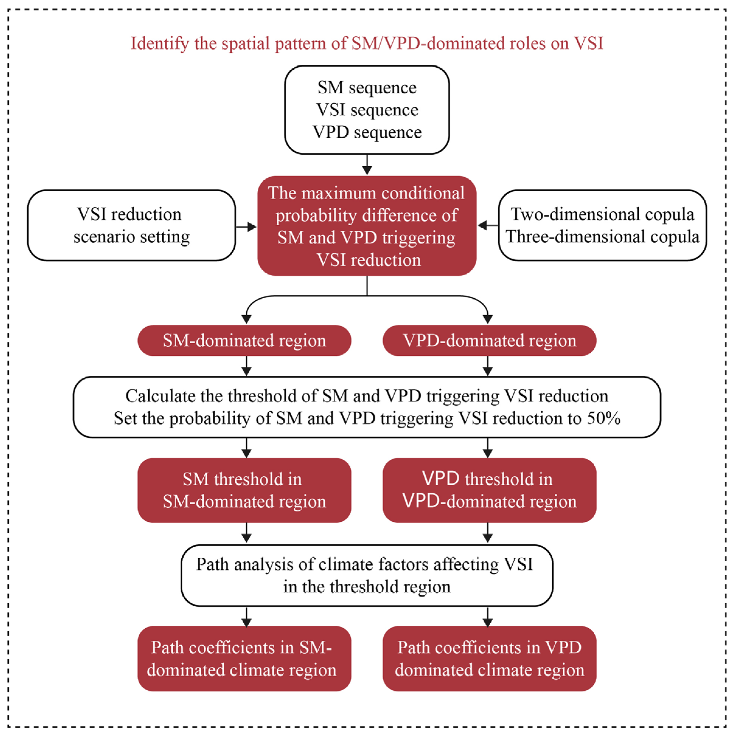
The methodological framework of this study consists of three principal steps (Figure 2). First, two- and three-dimensional Copula functions were applied to identify the spatial distribution patterns of vegetation productivity decline events dominated by single factors (either SM or VPD), and to quantify the joint probability of vegetation productivity (GPP, NDVI, SIF) decline under the compound stress. Second, based on the preceding analysis, the SM- and VPD-dominated regions were explicitly delineated, and the respective critical thresholds triggering vegetation productivity decline within each region were quantified. Third, Pearson correlation coefficients between vegetation productivity and SM/VPD were calculated to assess their linear relationships. Furthermore, a path analysis model was constructed to reveal the direct and indirect impact mechanisms of climatic factors on vegetation productivity. For clarity of expression, GPP, SIF, and NDVI are hereinafter collectively referred to as VSI.

2.3.1. Two-Dimensional (2D) Copula Statistical Modeling

The maximum conditional probability of VSI reduction under single-variable dominated mechanisms (i.e., SM or VPD) was further investigated by the 2D Copula method [27]. Copulas construct multivariate distribution functions by linking the marginal distributions of multiple variables, revealing the dependence structure between them [28]. This method effectively integrates dependence information and analyzes the dependence structure, particularly under extreme conditions [29]. Therefore, Copulas not only facilitates the assessment of VSI decline risk induced by low SM and elevated VPD, but also enables the calculation of SM and VPD thresholds under specific VSI decline scenarios. To this end, multiple bivariate Copula functions were employed in this study to quantify the dependence between VSI and SM/VPD (Equations (1) and (2)).

$$F_{SM,VSI}(SM, VSI)=C \left(F_{SM}\right(SM), F_{VSI}(VSI\left)\right)$$

(1)

$$F_{VPD,VSI}(VPD, VSI)=C \left(F_{VPD}\right(VPD), F_{VSI} (VSI\left)\right)$$

(2)

where F_SM, F_VPD, and F_VSI denote the marginal distributions of SM, VPD, and VSI, respectively, selected from seven candidate distribution functions through the Kolmogorov–Smirnov test for goodness-of-fit screening and the minimum Akaike Information Criterion (AIC) for final optimal selection; F_SM,VSI and F_VPD,VSI represent the joint distributions of (SM, VSI) and (VPD, VSI), respectively; C() signifies the Copula function, obtained from five candidate Copula types (Gaussian, t, Gumbel, Clayton, and Frank) in accordance with the Akaike Information Criterion (AIC). The selection of the optimal marginal distribution and Copula family for each grid cell was performed independently following the Akaike Information Criterion (AIC). Detailed statistics on the selection frequency and the results for each grid are provided in the Supplementary Materials (the CSV files: table1_marginal_selection(Group1).csv and table2_best_copula_2d(Group1).csv). The goodness-of-fit of the selected Copula models was validated by Probability Integral Transform (PIT) plots (Figure S5 in the Supplementary Information).

The Copula-based conditional probability functions were utilized to separately examine the impacts of SM and VPD on VSI (Equations (3) and (4)). The vegetation productivity reduction is identified when VSI falls below the 40th percentile of the decreasing VSI sequence during the study period.

$$P(VSI\le {VSI}^{\ast } |SM\le {SM}^{\ast })={\displaystyle \frac{P(VSI\le {VSI}^{\ast }, SM\le {SM}^{\ast })}{P(SM \le {SM}^{\ast })}}={\displaystyle \frac{F_{SM,VSI} ({SM}^{\ast }, {VSI}^{\ast })}{F_{SM}\left({SM}^{\ast }\right)}}$$

(3)

$$\begin{array}{ll}P(VSI\le {VSI}^{\ast }|VPD>{VPD}^{\ast })& ={\displaystyle \frac{P(VSI\le {VSI}^{\ast },VPD>{VPD}^{\ast })}{P(VPD>{VPD}^{\ast })}}\\ & ={\displaystyle \frac{F_{VSI} \left({VSI}^{\ast }\right)-F_{VPD,VSI}({VPD}^{\ast }, {VSI}^{\ast }) }{1-F_{VPD}\left({VPD}^{\ast }\right)}}\end{array}$$

(4)

$$P_{SM}=max\left(P\right(VSI\le {VSI}^{\ast }|SM\le {SM}^{\ast }))$$

(5)

$$P_{VPD}=max\left(P\right(VSI\le {VSI}^{\ast }|VPD>{VPD}^{\ast }))$$

(6)

where VSI* represents the defined level of VSI reduction, such as VSI^40th; SM* and VPD* embody the target SM and VPD values corresponding to the maximum conditional probability of VSI reduction induced by SM and VPD, respectively, i.e., P_SM and P_VPD (Equations (5) and (6)). SM* and VPD* can be calculated iteratively, ranging from the maximum to the minimum value of each pixel, with iteration steps of 0.01 m³/m³ and 0.01 hPa, respectively.

2.3.2. Three-Dimensional (3D) Copula Statistical Modeling

In this section, the spatial distribution patterns under compound stress conditions, defined by low SM and high VPD, were investigated by a three-dimensional (3D) Copula method. Co-occurrence of low SM and high VPD was observed under extreme drought conditions [7]. The probability of VSI reduction under the combined effects was analyzed by the classical Vine Copula (C-vine copula) method [14]. Subsequently, the 3D Copula model [13] served for the calculation of the probability of VSI decline under compound extreme conditions of low SM and high VPD, specifically when SM ≤ SM^10th and VPD > VPD^90th (Equations (7) and (8)).

$$F_{SM,VSI,VPD}(SM, VSI, VPD)=C_{SM,VSI,VPD} (F_{SM} (SM),F_{VSI} (VSI), F_{VPD}(VPD\left)\right)$$

(7)

$$\begin{array}{ll}{P}_{SM\&VPD}& =P(VSI\le {VSI}^{\ast },VPD>{VPD}^{90th},SM\le {SM}^{10th})\\ & ={\displaystyle \frac{C_{SM,VSI,VPD} (VSI\le {VSI}^{\ast },VPD>{VPD}^{90th},SM\le {SM}^{10th})}{P(VPD>{VPD}^{\ast },SM\le {SM}^{\ast })}}\\ & ={\displaystyle \frac{C(VSI\le {VSI}^{\ast }, SM\le {SM}^{10th})-C_{SM,VSI,VPD}(VSI\le {VSI}^{\ast },VPD\le {VPD}^{90th},SM\le {SM}^{10th})}{F_{SM}\left({SM}^{10th}\right)-C(VPD\le {VPD}^{90th}, SM\le {SM}^{10th})}}\end{array}$$

(8)

where F_SM,VSI,VPD represents the joint distribution of SM, VSI, and VPD; C_SM,VSI,VPD() denotes the C-vine copula dependence structure among VSI, VPD, and SM; P_SM&VPD signifies the conditional probability of VSI reduction when SM ≤ SM^10th and VPD > VPD^90th.

The application of the C-vine copula model involves several simplifying assumptions. First, the C-vine structure was selected because its star-like decomposition intuitively reflects the ecological mechanism of two stressors (SM and VPD) jointly impacting a central response variable (VSI). Second, the model relies on the standard “simplifying condition” for computational tractability. With the Akaike Information Criterion (AIC) as the primary selection criterion, the family for each pair-copula and the final C-vine structure were selected in a data-driven manner to ensure flexibility. Furthermore, the Bayesian Information Criterion (BIC), which penalizes complexity more heavily, was also calculated and reported for a more comprehensive assessment. The detailed AIC and BIC values (the CSV file: table3_vine_cvine_results(Group1).csv in the Supplementary Materials) confirm the robustness of our model selection.

2.3.3. Identification of the Spatial Distribution of SM/VPD-Dominated Regions

The 2D Copula method was adopted to analyze the spatial distribution of SM/VPD-dominated regions. P_diff denotes the difference between P_SM and P_VPD (Equation (9)). If the P_diff value for a grid cell is positive, SM more greatly impacts VSI reduction compared with VPD, and the cell is classified as an SM-dominated region; conversely, the cell can be classified as a VPD-dominated region.

$$P_{diff}=P_{SM}-P_{VPD}$$

(9)

2.3.4. Determination of Critical Thresholds for SM and VPD Within SM/VPD-Dominated Regions

The critical point was defined as the SM and VPD value at which the conditional probabilities (P(VSI ≤ VSI* | SM ≤ SM*) and P(VSI ≤ VSI* | VPD > VPD*)) that VSI decreases due to a reduction in SM or an increase in VPD first reach 50% [21].

Additionally, an iterative approximation method was employed to precisely quantify these thresholds. In SM-dominated regions, the SM value was progressively decreased from its maximum observed value, with a step size of 0.01 m³/m³. When the value of the aforementioned conditional probability was ≥0.5, the iteration process was terminated, and the SM value at that point was adopted as the threshold. While a similar computational procedure was applied for VPD-dominated regions, the VPD value was progressively increased from its minimum value until the corresponding conditional probability satisfied the criterion.

Grid cells for which the aforementioned thresholds were successfully calculated constitute the “SM/VPD threshold region”. In these regions, the high or low values of the thresholds reflect the vegetation’s sensitivity to different levels of water stress. A higher SM threshold in a particular grid cell indicates that the vegetation in this area is more sensitive to SM deficits; a lower VPD threshold specifies that local vegetation is more prone to stress due to rising atmospheric drought conditions.

2.3.5. Analysis of Correlation and Mechanisms of Climatic Factor Impacts on VSI

Calculating the Pearson correlation coefficient between the VSI, SM, and VPD is a crucial step in studying their interactions. The Pearson correlation coefficient interprets the linear relationship between two variables, with a value in the range of [−1–1], indicating the degree of complete negative to complete positive correlation [30]. The interrelationships between these variables can be more deeply understood by calculating the following correlation coefficients. r(VSI, SM) measures the relationship between VSI and soil moisture, reflecting the impact of SM on vegetation health [7]. r(VSI, VPD) enables the analysis of the relationship between VSI and VPD, as well as the evaluation of the impact of atmospheric humidity on plant transpiration and health. r(SM, VPD) reveals the interaction between SM and VPD, assisting in exploring the relationship between water supply and atmospheric demand. These correlation coefficients facilitate a comprehensive understanding of the impact of environmental factors on vegetation status, thereby supporting ecological and climate change research.

SEM [30,31] was utilized to elucidate the influence pathways and underlying mechanisms of climate factors on the VSI. It is a multivariate statistical method combining the advantages of factor analysis and path analysis and can effectively elucidate the direct and indirect causal relationships among elements in different climate zones by examining the covariance matrix of the variables. Thus, it is commonly applied in biological and ecological research [32].

Within this framework, our research group constructed an SEM encompassing seven core variables: TP, SM, SSR, VPD, RH, TM, and the final response variable, VSI.

The data were processed in two main steps to satisfy the prerequisites for the model analysis. First, the inherent linear trend of each variable at each grid cell was removed through the residuals from an ordinary least squares (OLS) regression against time. This ensures that the relationships explored were not confounded by long-term secular trends. Subsequently, these detrended time series were z-score standardized before being applied in the SEM analysis to render the path coefficients comparable across variables with different units and variances.

A path analysis approach was employed within the framework of Structural Equation Modeling (SEM). Individual path coefficients were estimated using Ordinary Least Squares (OLS) regression. The overall model fit was evaluated by comparing the observed and model-implied covariance matrices, with fit indices—including χ², Comparative Fit Index (CFI), Tucker-Lewis Index (TLI), Root Mean Square Error of Approximation (RMSEA), and Standardized Root Mean Square Residual (SRMR)—calculated under the Maximum Likelihood (ML) estimation method. To examine potential multicollinearity among the predictor variables, Variance Inflation Factors (VIFs) were computed for each variable across all nine dataset. Our analysis reveals that all VIF values were consistently well below the common threshold of 5.0, confirming that multicollinearity was not a significant concern. The detailed results for Group 1 (NIRv-GPP with ERA5-Land) are presented as a representative example in Supplementary Tables S2–S4.

The statistical significance of the path coefficients was assessed based on p-values, denoted by asterisks: ** for p < 0.01 and * for 0.01 ≤ p < 0.05. Furthermore, a robust sample size for all scenarios was guaranteed following recommendations from relevant studies [33]. The effective sample size for each SEM was calculated by pooling all valid grid cells within a given climate zone across all months of the growing season (May–September) during the study period. This is the product of the number of grid cells and the number of monthly observations. For example, the analysis over the 2000–2018 period includes 95 monthly observations per grid cell (19 years × 5 months/year) for a climate zone containing 80 valid grid cells, with a total sample size of 7600 (80 × 95). Therefore, the sample sizes for all our models were in the thousands to tens of thousands, substantially greater than the minimum required for robust SEM analysis, allowing for the reliability of our path analysis results.

The selection of variables in the SEM was based on their physiological relevance within the climate-vegetation system and their identifiable causal pathways. The model was designed to disentangle the crucial linkages from climatic drivers to vegetation productivity. TM, TP, and SSR were incorporated as the core climatic drivers, representing energy balance, water input, and photosynthetic energy supply, respectively. They exert fundamental controls on plant physiological processes. RH was included as a vital bridge between the atmosphere and the soil, as it directly determines VPD (that is, regulating stomatal behavior and transpiration) and modulates SM dynamics through its influence on evaporation. Thus, SM and VPD were defined as key mediating variables that respond to climatic forcing and directly affect vegetation productivity. Although wind speed and atmospheric CO₂ concentration can also influence vegetation function, their effects at the regional scale considered in this study are primarily mediated through variables such as VPD, SM, or TM. Moreover, consistent high-quality data for these variables across multiple climate zones were not readily available. Therefore, they were excluded from the current model framework. Overall, the selected variable set (TM, TP, SSR, RH, SM, VPD) forms a mechanistically coherent chain linking climatic forcing to vegetation responses while maintaining strong statistical identifiability within the multi-source datasets employed. Future research could expand the model to incorporate additional variables such as wind speed and CO₂, when data availability permits, to further refine the understanding of vegetation response mechanisms.

3. Results

3.1. Copula Statistical Modeling

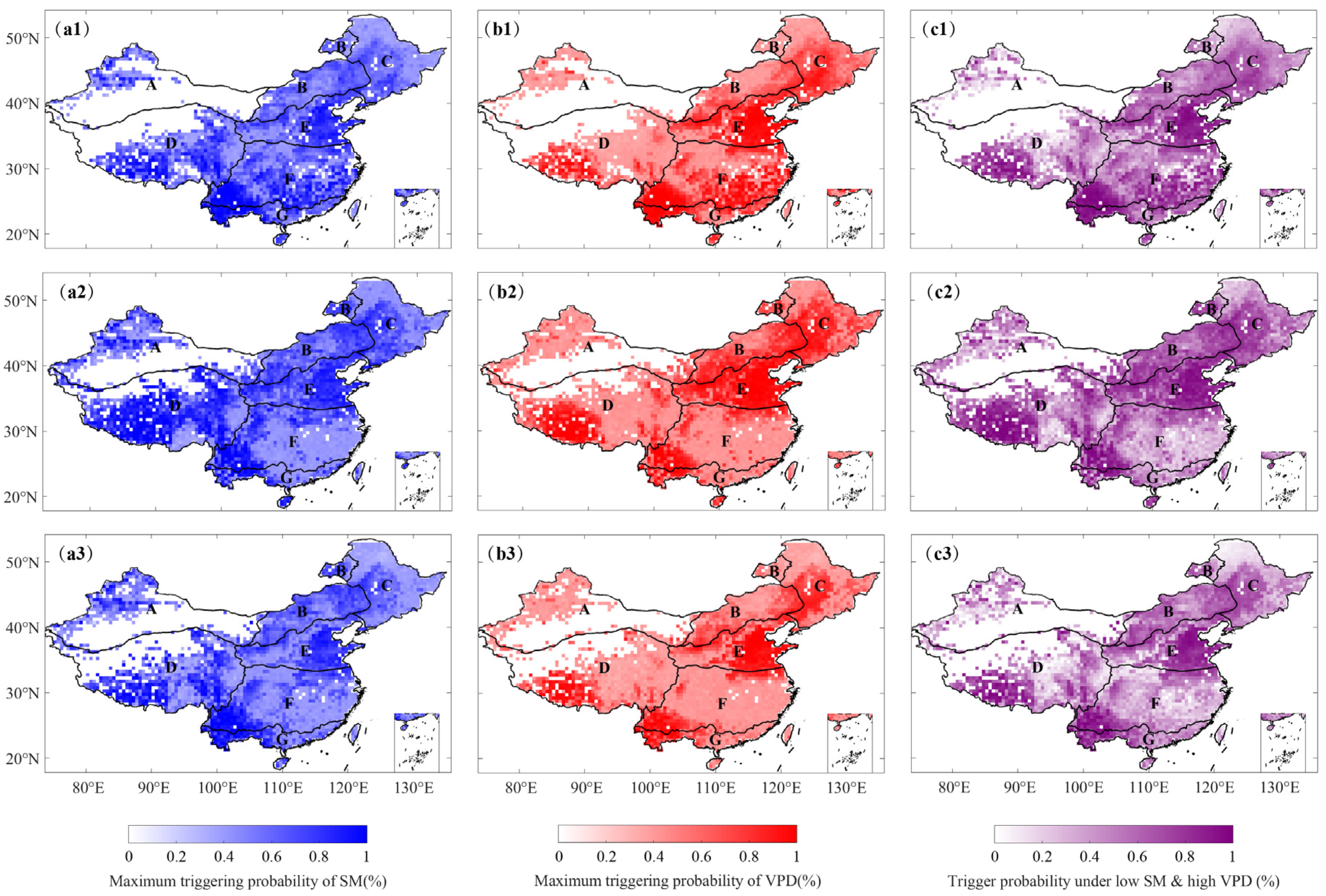
P_SM was ascertained to quantify the impact of SM supply on VSI decline. The spatial distribution of P_SM (Figure 3(a1–a3)) was similar to the distribution pattern of high P_SM&VPD (Figure 3(c1–c3)). Regarding water stress arising from atmospheric evaporative demand, the maximum conditional probability of VSI decline is triggered by VPD (P_VPD)(Figure 3(b1–b3)). The analysis of P_SM and P_VPD reveals that multiple regions in China exhibited high sensitivity to single-factor droughts. Notably, the spatial distribution of P_SM and P_VPD is highly similar to that of the correlations between VSI and SM, and between VSI and VPD, respectively, as will be discussed and shown later in Figure 6a,b. In regions with high P_SM, VSI was significantly positively correlated with SM; in regions with high P_VPD, VSI exhibited a significant negative correlation with VPD.

The conditional probability of VSI decline, P_SM&VPD, was investigated under the concurrent conditions of low SM (SM ≤ SM^10th) and high VPD (VPD > VPD^90th) (Figure S1(c1–c9)). Within the same dataset groups, high P_SM&VPD (Figure S1(c1–c9)) exhibited a spatial distribution pattern similar to high P_SM (Figure S1(a1–a9)) and high P_VPD (Figure S1(b1–b9)). The spatial distribution patterns of the VSI decline triggering probability under low SM and high VPD conditions, derived from different dataset groups, were also similar (such as Figure S1(c1,c3,c4,c6,c7,c9)). Nonetheless, the magnitude of probability change was smaller when the Vegetation Remote Sensing Index was NDVI (Figure S1(c2,c5,c8)), presenting a smoother spatial distribution trend. The hotspot areas were concentrated in the southwestern part of Zone C, the eastern part of Zone E, the southwestern part of Zone D, and the southwestern parts of Zones F and G. In other words, the areas where VSI reductions are driven solely by low SM or high VPD tend to be more vulnerable to the combined impacts of compound extreme events.

3.2. Determination of Critical Thresholds for SM and VPD Within SM/VPD-Dominated Regions

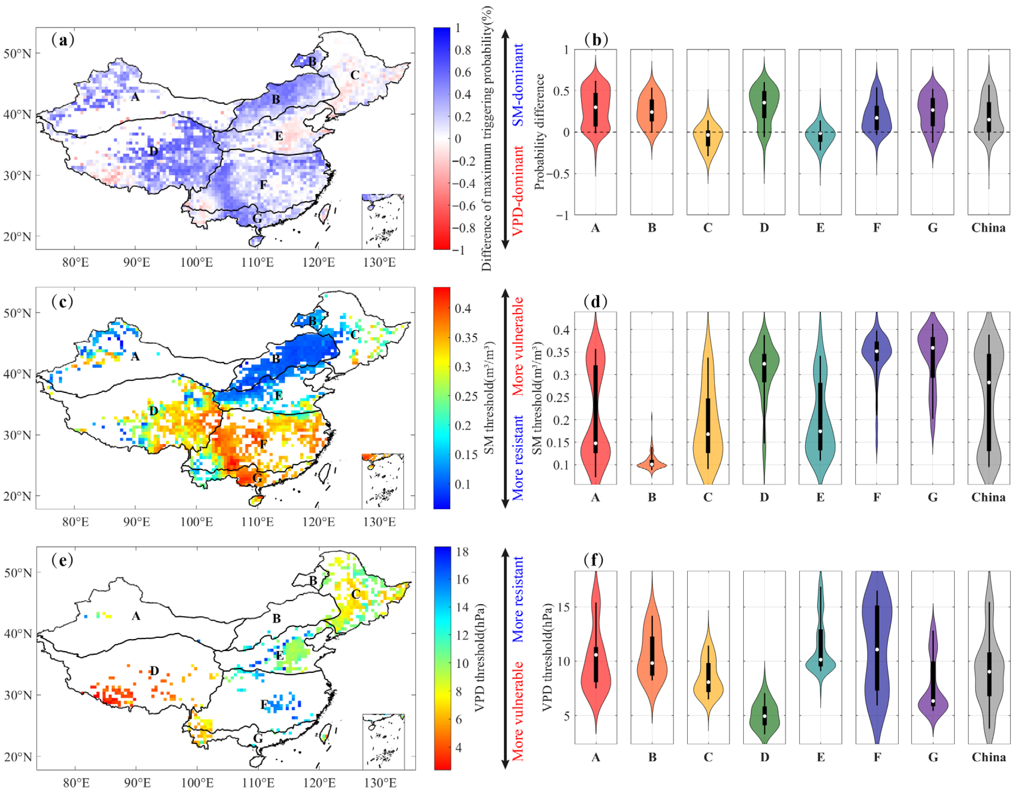
The spatial patterns in Figure 4a,b reflect that arid/semi-arid regions (Zones A, B, and D) exhibit stronger SM dominance, while the semi-humid regions (Zones C and E) are characterized by enhanced VPD dominance. This pattern is strongly influenced by the local topography and climatic conditions. Zones C and E generally feature low and flat topography, with elevations mostly below 200 m. Heat accumulates easily in the open terrain, unobstructed by high mountains, and enables direct solar radiation to reach the surface, leading to rapid ground warming. Concurrently, low-altitude areas with higher air density and heat capacity trigger rapid warming during the day and slow cooling at night, resulting in a higher overall daily mean temperature. Higher temperatures indicate that the atmosphere has a greater capacity to retain water vapor. If humidity does not increase synchronously, the air’s dryness (VPD) rises rapidly. Although plateaus or mountainous regions also warm up during the day, the thin air allows radiation to dissipate easily, bringing about rapid nighttime cooling. Consequently, the average temperature is not as high as in the plains, and VPD does not fluctuate as dramatically. In summary, the controlling effect of VPD becomes more significant in these flat, high-temperature semi-humid regions, whereas the limitation imposed by SM on vegetation physiology is relatively weakened. Notably, this conclusion was highly consistent across the analyses of all nine datasets, further supporting the stability of the SM and VPD dominance patterns in varying climate zones. SM remains the dominant factor causing VSI decline in the humid regions (Zones F and G), which are represented by plains and hills with abundant precipitation. Its influence is stronger than in the semi-humid regions but weaker than in the arid/semi-arid regions; conversely, the VPD-dominant influence is weaker than in the semi-humid regions but stronger than in the arid/semi-arid regions. Despite high annual precipitation, its seasonal distribution is uneven (such as influenced by the monsoon climate), and short-term droughts can still lead to rapid SM decline. Furthermore, in hilly areas, the topography leads to poor soil water-holding capacity, and moisture is easily lost from slopes. In contrast, plains may experience localized waterlogging due to poor drainage, both of which affect SM effectiveness. During high-temperature weather, VPD can still rise briefly, such as on summer afternoons, even if air humidity is high, imposing intermittent stress on vegetation.

The SM-dominant regions are primarily located in Zones A, B, D, F, and G (Figure 4a). Notably, the impact of VPD on VSI decline exhibits opposing trends under different climatic conditions. The dominant effect of VPD (i.e., its negative effect) is essentially concentrated in Zones C and E, particularly in the low-lying and flat regions with elevations below 200 m.

The SM/VPD thresholds and their relative thresholds were determined within the SM/VPD-dominant regions, defined as the point where P_SM and P_VPD reached 50%. The SM and VPD thresholds were successfully identified within 74.69% and 87.63% of their respective dominant regions. The SM threshold and its relative threshold demonstrate distinct spatial differences among climate zones, with thresholds in Zones D, F, and G generally higher than those in Zones A, B, and E (Figure 4c,d). The spatial distribution of the SM threshold did not present a simple north-south gradient but was significantly influenced by climate type. Since vegetation in the humid regions (Zones F, G) and the plateau temperate semi-arid region (Zone D) is more sensitive to SM variations, it displays a higher SM threshold. However, vegetation in arid and semi-arid regions (Zones A, B) is more drought-tolerant, resulting in a relatively lower threshold. Moreover, the semi-humid region (Zone E) falls at an intermediate level. This pattern illustrates climate-specific differences in how vegetation responds to drought stress across the various climate zones. The strong agreement in spatial patterns identified by all nine datasets further reinforces the statistical reliability and broad applicability of this finding. The VPD threshold is predominantly concentrated in Zone C (mid-temperate semi-humid), Zone D (plateau temperate semi-arid), and Zone E (warm-temperate semi-humid), specifying pronounced regional contrasts. In other words, the vegetation’s response to atmospheric drought (VPD) is considerably dependent on geography and climate. Specifically, the VPD threshold in Zone D (plateau) is the lowest. This region features high altitude, low air pressure, and thin air. While the absolute VPD value may not be large, its stress effect on vegetation is highly pronounced [34]. This is because plateau vegetation, which typically grows slowly and has a weaker water regulation capacity, exhibits rapid physiological responses (such as stomatal closure and reduced transpiration rates) even under relatively mild atmospheric drought [6]. As a result, its ecological function remarkably declines. The threshold in Zone C, mainly appearing in mid-temperate plains, is higher than that in Zone D. The threshold in Zone E, mostly distributed in warm-temperate plains, is higher than that in Zone D and slightly higher than that in Zone C. This implies that vegetation in these regions can tolerate higher levels of VPD stress. The multi-dataset results collectively reveal that the spatial variability of the VPD threshold profoundly reflects the significant climatic and topographic dependency of vegetation’s response to atmospheric drought (Figure S2 in the Supplementary Information).

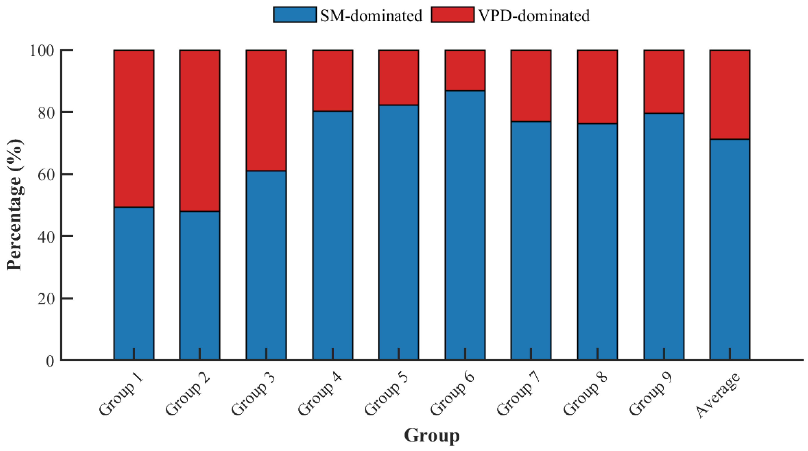
The difference P_diff between P_SM and P_VPD was considered to confirm SM-dominant and VPD-dominant regions. Overall, SM remains the dominant factor constraining terrestrial vegetation productivity across China. Across all dataset groups, the average dominant proportion of SM was 71.16%, which was significantly higher than the 28.84% average for VPD (Figure 5). While different datasets were employed to estimate vegetation productivity and drought stress, the vast majority of sources (7 out of 9 datasets) yielded a consistent and robust conclusion. Specifically, SM is a more dominant limiting factor for vegetation productivity than atmospheric drought across China. This finding significantly enhances the reliability of the study’s conclusions.

The results from the six independent datasets of Groups 4 to 9 were highly consistent, and their SM-dominant proportions were concentrated within a narrow range of 76.20–86.88%. The results from Groups 1, 2, and 3 constituted the “uncertainty boundary” for the study’s conclusions. These groups’ results reflect that indicate that the influence of VPD was enhanced to a level comparable to, or even slightly higher than, that of SM when SM and VPD data were sourced from the ERA5-Land reanalysis dataset. In other words, the choice of data source does not undermine the core finding that “SM remains the dominant limitation on vegetation productivity across China,” even though it may influence the strength of the conclusion.

With the purpose of further investigating this dominance from the perspective of joint extreme events, the co-occurrence risk of extreme vegetation productivity decline under extreme soil or atmospheric drought was quantified by calculating tail dependence coefficients (λ) from the fitted Copula models. The lower tail coefficient (λ₁) for SM–GPP represents the conditional probability of GPP being extremely low given SM is extremely low; the upper tail coefficient (λ_u) for VPD–GPP indicates the probability of GPP being extremely low given VPD is extremely high. Complete results are summarized in

Table 2. Tail dependence summary for Group 1.

Metric	Mean	Std	Min	Max	N
Lower Tail (SM-GPP)	0.067	0.158	0.000	0.835	2657
Upper Tail (SM-GPP)	0.047	0.101	0.000	0.592	2657
Lower Tail (VPD-GPP)	0.022	0.087	0.000	0.691	2657
Upper Tail (VPD-GPP)	0.005	0.033	0.000	0.413	2657

.

According to Table 2, the mean λ₁ for SM–GPP was 0.067, specifying a 6.7% probability of extreme GPP decline under extreme soil drought. In contrast, the mean λ_u for VPD–GPP was only 0.005, implying only a 0.5% probability under extreme atmospheric drought. This order-of-magnitude difference (6.7% vs. 0.5%) suggests that vegetation is over ten times more likely to experience concurrent extreme declines with soil drought than with atmospheric drought. These results further support the dominance of SM over VPD in driving vegetation stress under extreme drought conditions.

3.3. Correlation Analysis Between VSI and SM/VPD and Mechanism Study of Climate Impacts on Vegetation Productivity

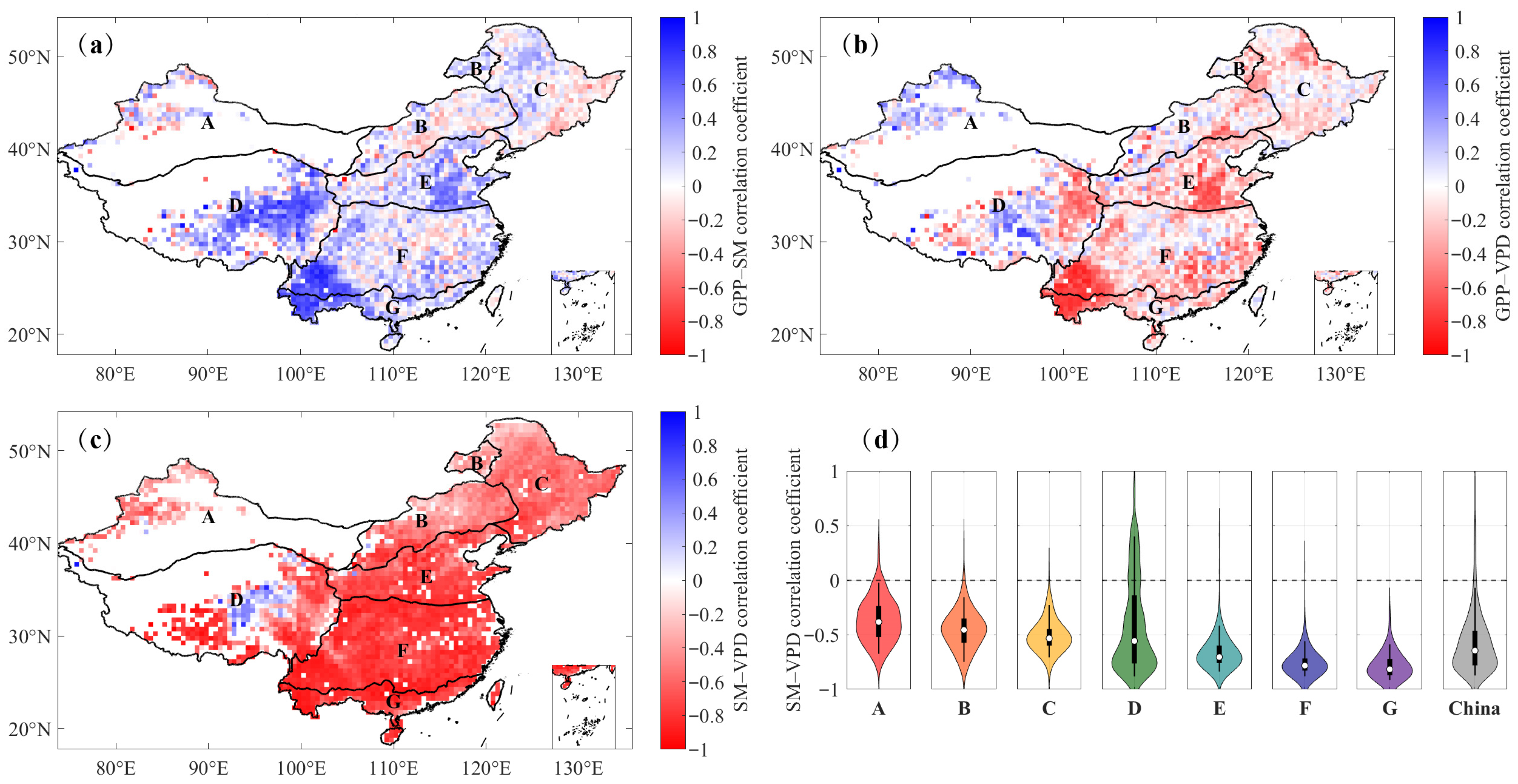
r(VSI, SM) demonstrates a strong positive correlation in most regions, indicating that SM is strongly related to the VSI in these areas. The spatial distribution of r(VSI, VPD) presents a negative correlation in most regions. In other words, increased VPD is accompanied by decreased VSI, reflecting that VPD exerts an inhibitory effect on vegetation photosynthetic activity. The spatial distribution of r(SM, VPD) reveals a negative correlation between SM and VPD in most regions, particularly in Zones E, F, and G, in which elevated VPD is typically associated with a reduction in soil moisture. Nonetheless, a clear positive correlation between SM and VPD is observed in the eastern part of Zone D. This anomaly might stem from the region’s unique climatic and geographical conditions. In this region (a plateau temperate semi-arid zone), the average elevation typically exceeds 4000 m. Low air pressure, thin air, and seasonal glacial meltwater collectively perturb the local evapotranspiration process [35]. Concurrently, precipitation is concentrated in summer, and monsoon-transported water vapor brings abundant precipitation to the eastern part, whereas the central and western parts remain relatively arid. These unique topographic and climatic conditions collectively shape the distinct SM-VPD coupling relationship in this zone. Moreover, this spatial pattern was consistently validated across the analyses of all nine independent datasets (Figure S3 in the Supplementary Information).

Figure 6. Spatial patterns of the Pearson correlation coefficients among VSI, SM, and VPD: (a) r(VSI, SM), (b) r(VSI, VPD), and (c) r(SM, VPD). (d) Violin plots of the r(SM, VPD) distribution across different climate zones. Results are illustrated only for Group 1. The analysis period for this group is 2000–2018. The complete dataset for all nine groups can be found in Figure S3 in the Supplementary Information.

Figure 6. Spatial patterns of the Pearson correlation coefficients among VSI, SM, and VPD: (a) r(VSI, SM), (b) r(VSI, VPD), and (c) r(SM, VPD). (d) Violin plots of the r(SM, VPD) distribution across different climate zones. Results are illustrated only for Group 1. The analysis period for this group is 2000–2018. The complete dataset for all nine groups can be found in Figure S3 in the Supplementary Information.

The violin plots illustrate the distribution of r(SM, VPD) across the different climate zones. Zones E (warm-temperate semi-humid), F (north-subtropical humid), and G (marginal-tropical humid) exhibit a strong negative correlation with a concentrated distribution, specifying a stable and significant SM–VPD relationship. This stable, strong negative correlation is likely associated with the more humid climatic background of these regions. The negative correlation in Zone A (mid-temperate arid), Zone B (mid-temperate semi-arid), and Zone C (mid-temperate semi-humid) is relatively weaker. The violin plots suggest that the correlation in Zones A, B, and C is weaker than that in Zones E, F, and G. The reasons for this result are detailed as follows. First, SM in Zones A and B is persistently low, with vegetation limited primarily by absolute SM deficits rather than VPD fluctuations, Second, SM has been near its lower threshold (such as the wilting point) even when VPD rises, causing the two factors to approach “decoupling”. Although episodic precipitation events can briefly elevate SM, the high evaporation rates in arid regions induce it to decline rapidly, disrupting the temporal consistency between SM and VPD. In the temperate monsoon climate zone (Zone C), sharp temperature increases or dry-hot wind events are common in spring and summer, bringing about rapid rises in VPD. Nevertheless, the correlation between the two is further weakened if SM is relatively ample at this time due to antecedent precipitation or snowmelt [36]. The violin plot for Zone D (plateau temperate semi-arid) exhibits a much broader distribution range, suggesting greater volatility in the SM–VPD correlation. This arises from the region’s complex environmental factors, including high elevation, low air pressure, thin air, and seasonal glacial meltwater, which collectively perturb the evapotranspiration process [12]. Concurrently, summer monsoon precipitation is extremely unevenly distributed spatially (concentrated in the east, while the central and western parts are arid). Furthermore, the interplay of topographic and monsoon factors provokes a considerably complex SM–VPD coupling relationship. As a result, the correlation varies within the region from significantly negative to significantly positive values, demonstrating high volatility and variations across space.

In summary, the correlation between SM and VPD exhibits significant differences in both strength and stability across climate zones. These differences reflect the distinct characteristics of each climate zone and the profound influence of climatic factors, such as humidity, elevation, and air pressure, on the SM–VPD interaction. The combined analysis of all nine datasets collectively validates that the SM–VPD coupling relationship differs significantly across diverse climatic backgrounds.

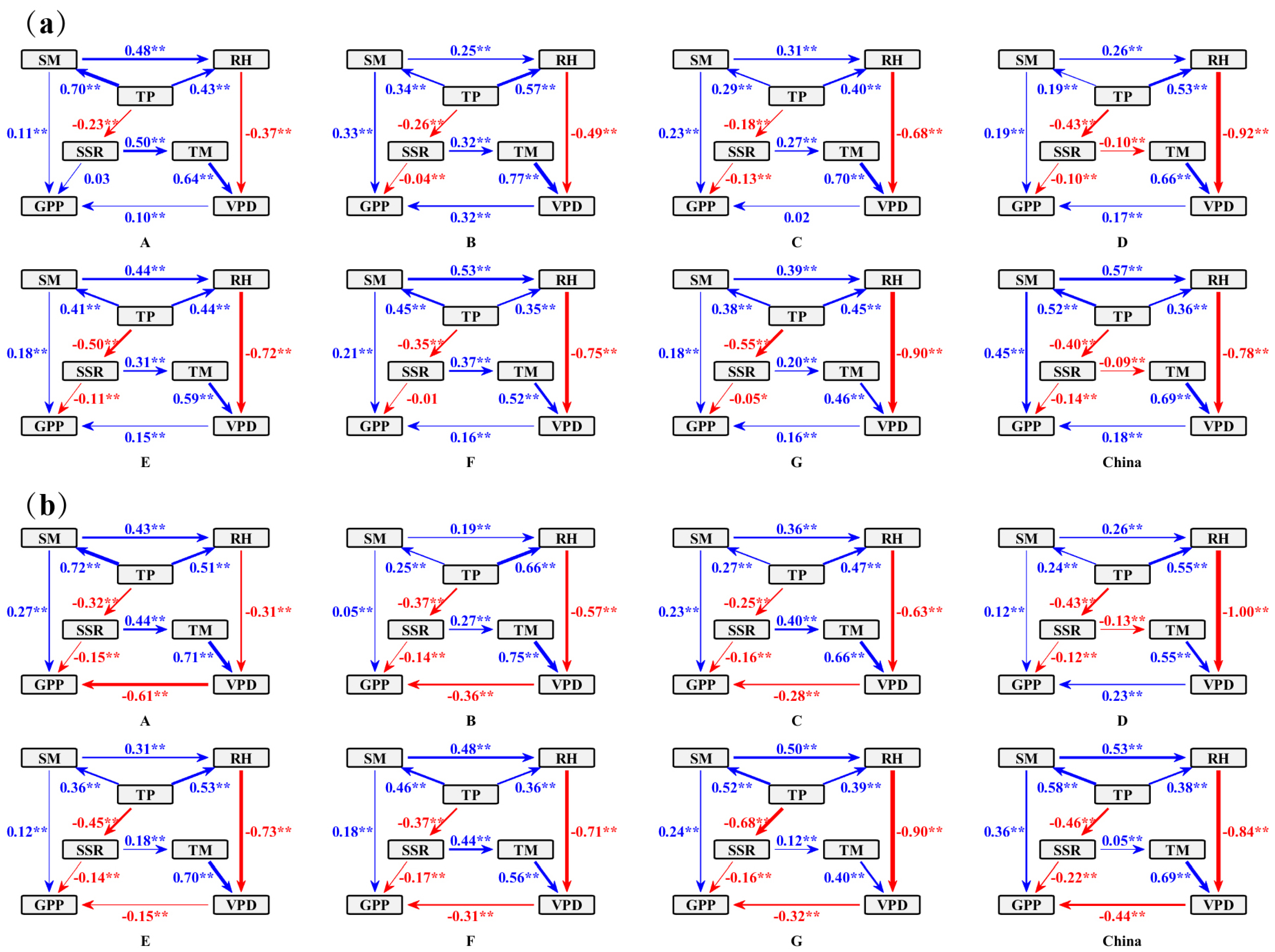
The effects of climate variables on VSI within the SM-threshold and VPD-threshold regions were analyzed by the SEM, as illustrated in Figure 7. The mechanisms by which climate variables affect VSI differ significantly between the two regions (Figure 7a,b). This disparity was consistently observed across the analyses of all nine datasets (Figure S4 in the Supplementary Information), confirming the robustness and universality of the findings. Specifically, the positive effect of SM on VSI (as measured by standardized path coefficients) in the SM-threshold regions is considerably stronger than that in the VPD-threshold regions. With the exception of Zone D, VPD exerted a negative effect on VSI in the VPD-threshold regions, and a positive path coefficient was uniformly observed in the SM-threshold regions, implying a more complex interaction. SSR more remarkably inhibits VSI in the VPD-threshold regions compared to the SM-threshold regions. These results align with previous studies [21].

The overall goodness-of-fit for each SEM was evaluated through standard indices, including the chi-square (χ²) test, CFI, TLI, RMSEA, and SRMR, to perform a comprehensive assessment of the models. The detailed results for Group 1 are presented as a representative example in the Supplementary Information (Table S5). Notably, several fit indices failed to meet the conventional thresholds for a “good fit”. This pattern was consistent across all nine data groups, confirming that it is a common, generally expected outcome when applying SEM to large and complex ecological datasets. This is because the high sensitivity of the χ² test to very large sample sizes can adversely affect other indices. Moreover, the primary objective of our SEM application was to test specific hypotheses about causal pathways through path analysis rather than to build a perfectly predictive model. Therefore, our interpretation rightly focuses on the significance, direction, and magnitude of the individual path coefficients illustrated in Figure 7. These coefficients provide robust and valuable mechanistic insights into the drivers of vegetation productivity, aligning with the central aims of our study.

4. Discussion

4.1. Dominant Roles of SM/VPD and Their Thresholds

A 2D/3D Copula framework was employed to quantify the relative contributions of soil drought and atmospheric drought to the reduction in VSI across China’s seven major climate zones during the study period. The results, derived from nine datasets, suggest that the conditional probability P_SM&VPD of VSI reduction triggered jointly by low SM and high VPD is spatially similar to the patterns of the single-factor-driven P_SM and P_VPD. The consistent spatial distribution trends of P_SM&VPD across multiple datasets specify a stable sensitivity of these regions to compound drought.

These hotspot regions are primarily concentrated in southwestern Zone C, eastern Zone E, southwestern Zone D, and the southwestern parts of Zones F and G. The regions with high P_SM coincide with the areas exhibiting a strong positive correlation between VSI and SM; the regions with high P_VPD correspond to areas featuring a strong negative correlation between VSI and VPD. Furthermore, the spatial patterns of P_SM and P_VPD are highly consistent with the VSI–SM/VPD correlation patterns in Figure 6, further corroborating the coupling relationship between dominant drought factors and vegetation stress response. From a plant physiological perspective, SM represents plant water availability. Thus, low SM directly restricts plant growth via hydraulic processes, inducing xylem cavitation and hindering transpiration [7,37]. Unlike the immediate stomatal regulation associated with VPD, the effect of SM on VSI typically presents a longer-term lagged effect [24,38]. Previous research findings also confirmed the critical role of SM on VSI in China [1,11]. The SM threshold varies across climate zones. Vegetation in Zones E and F is commonly adapted to higher precipitation and demonstrates low water use efficiency, manifested as a greater reliance on current-month precipitation and water extraction from shallow soil layers [39,40]. Consequently, VSI in these southern regions is more sensitive to reductions in SM. In Zone D (plateau temperate semi-arid), the seasonal regulation of water homeostasis by glacial meltwater is limited, regardless of suppressed evapotranspiration rates (due to high elevation, low air pressure, and thin air) [41]. Hence, this region is more sensitive to short-term SM fluctuations. In contrast, the plain areas of the transitional semi-humid zones (Zones C and E) are subjected to rapid heat accumulation. The open terrain and lack of mountain shading allow solar radiation to directly irradiate the surface, bringing about rapid surface warming. In low-altitude areas, higher air density and greater heat capacity contribute to rapid daytime temperature increases and slow nighttime cooling, resulting in higher daily mean temperatures. As temperature increases, the atmosphere accommodates a greater amount of water vapor; if humidity does not rise synchronously, the air’s dryness (VPD) rapidly increases. VPD dominates the VSI reduction process in these regions. In these areas, the VPD threshold is low, making VPD the key limiting factor for photosynthesis, while the effect of SM is comparatively weak. To sum up, southwestern Zone C and similar hotspot areas exhibit strong sensitivity to rapid increases in atmospheric dryness, implying a heightened risk of vegetation stress under abrupt warming or low-humidity conditions. Such conditions may exacerbate agricultural water stress and elevate crop yield risks, implying that it is urgent to monitor compound drought indicators for early warning and regional drought management.

SM dominated the VSI reduction in 71.16% of vegetation pixels (Figure 5), especially pronounced in arid/semi-arid zones (A, B, D) and the hot-humid southern zones (F, G). The dominance of VPD was primarily concentrated in the semi-humid plains (Zones C and E) at elevations below 200 m. Our multi-dataset synthesis reveals that SM is the dominant factor constraining vegetation productivity across approximately 71.16% of China’s vegetated area. This proportion aligns closely with findings from recent independent studies. At the global scale, Liu et al. (2020) [7] reported that SM dominates ecosystem dryness stress over >70% of vegetated land areas. More specifically for China, Wang et al. (2025) [21] utilized a similar Copula-based approach but different GPP data and found SM dominance over 71.06% of the country’s vegetation regions. The remarkable consistency among these estimates (derived from different methods (binning vs. Copula), different primary data, and slightly different study periods) provides strong external validation for the robustness of the spatial dominance pattern we identified.

The threshold analysis reveals significant inter-zonal differences. Specifically, the average SM threshold for Zones D (plateau temperate semi-arid), F (north subtropical humid), and G (marginal tropical humid) was approximately 0.33 m³/m³; the lowest thresholds were observed in Zones A (mid-temperate arid) and B (mid-temperate semi-arid), averaging approximately 0.13 m³/m³. Regarding VPD thresholds, Zone D (plateau temperate semi-arid) exhibited the lowest value; the threshold in Zone C (mid-temperate semi-humid), primarily found in the middle temperate plain regions, was higher than that in Zone D; the threshold in Zone E (warm-temperate semi-humid) was higher than that of Zone D and slightly higher than that of Zone C, demonstrating that the vegetation in this region can tolerate higher VPD stress.

4.2. Underlying Mechanisms of SM/VPD Dominance and Thresholds

Water stress arises from the low soil water supply coupled with high atmospheric evaporative demand, while precipitation is the critical means for natural water replenishment [7,42]. The energy available to plants is primarily derived from photosynthetically active radiation, which constitutes the main component of SSR [43]. This study suggests that changes in VSI are predominantly governed by climate-driven variations in SM and VPD, a pattern consistent in varying climate zones and VSI datasets. Typically, VSI is directly influenced by both the water stress from SM and VPD and the energy limitations from SSR. In the regions where SM is the dominant factor (i.e., SM-threshold regions), VPD is generally not a constraint and may exert a promotive effect on VSI [21]. This is because such regions (such as Zones D, F, and G) have high SM thresholds, where a moderate increase in VPD facilitates CO₂ uptake and transpiration under open stomatal conditions, thereby enhancing VSI. In the areas with low VPD thresholds, namely, the plains of semi-humid zones (C and E) where VSI is highly sensitive to VPD increases, a rise in VPD exerts a direct inhibitory effect on photosynthesis. The mechanism for this phenomenon is closely associated with the local environment. Specifically, the open terrain and lack of mountain shading allow solar radiation to stimulate rapid surface warming. Coupled with the greater heat capacity of air in low-altitude regions, this brings about rapid daytime warming and slow nighttime cooling, maintaining higher daily mean temperatures. The air’s dryness (VPD) rapidly increases when temperatures rise without a synchronous increase in humidity [6,8]. Furthermore, SSR negatively impacts VSI during the growing season, particularly during periods of intense radiation. Excessive SSR can damage photosystem II (PSII), induce photooxidative stress, and thus restrict plant growth [44].

4.3. Uncertainty in the Dominant Drivers of VSI Reduction

Although SM was identified as the leading contributor to VSI reduction [1,35], its contribution is still subject to certain uncertainties. First, systematic discrepancies exist among multi-source SM datasets (such as ERA5-Land, GLEAM, and GLDAS). Particularly, the biases in estimating deep-layer SM and capturing drought extremes may lead to errors (over- or underestimation) in the estimated area of SM-dominated regions. Second, our analysis did not incorporate the potential impacts of anthropogenic activities. Interventions such as irrigation, afforestation (or “Grain for Green”), and groundwater extraction can alter the natural spatiotemporal distribution of soil moisture, leading to drifts in local SM thresholds and subsequently changes in vegetation response patterns to SM stress [45]. For instance, widespread irrigation in arid and semi-arid agricultural areas can mask the natural stress from low soil moisture, lessening the apparent dominance of SM in those specific grid cells. Conversely, land cover changes alter local evapotranspiration dynamics, thereby shifting the balance between SM and VPD control. These factors reflect a limitation and a crucial direction for future research. Furthermore, the 2D Copula model employed in this study was not designed to capture interactions with other climate factors, such as radiation. This may provoke an underestimation of the nonlinear vegetation response mechanisms driven by multiple factors.

A key strength of this study is that our multi-dataset framework allows for the explicit quantification of these data-driven uncertainties. Thus, the variability observed in the estimated dominance of SM and VPD across Groups 1–9 is not just a limitation, but a central finding of our cross-validation, particularly when a comparison is performed between the results derived from different reanalysis products such as ERA5-Land, GLDAS, and the observation-based CRU dataset. For instance, Groups 1–3 (which relied on ERA5-Land for SM and VPD) exhibited a higher VPD influence compared to other dataset groups. This discrepancy stems from systematic biases in the representation of deep-layer SM and the characterization of drought extremes across datasets. ERA5-Land, featuring higher spatial resolution and assimilation of satellite observations, can better capture short-term atmospheric aridity signals, thereby enhancing the apparent role of VPD in vegetation stress. In contrast, GLDAS Noah LSM (which relies more on land surface modeling) emphasizes SM dynamics in deeper layers, leading to a stronger SM dominance signal. The CRU dataset, as an interpolated product based on station data at a coarser 0.5° resolution, can produce a spatially smoother VPD field. This smoothing effect can dampen localized extremes in atmospheric aridity, leading to a lower estimated VPD influence compared to the higher-resolution ERA5-Land product. While our cross-validation across all nine dataset groups provides a robust consensus on the overall dominance of SM across China, these observed variations among ERA5-Land, GLDAS, and CRU-driven results underscore the importance of data source selection in regional drought studies. Thus, future work could benefit from targeted sensitivity analyses that isolate the influence of specific dataset characteristics, such as vertical soil layer representation, assimilation inputs, and temporal smoothing, on the estimation of SM and VPD thresholds.

In addition to data source uncertainty, the choice of percentile thresholds (i.e., VSI ≤ VSI^40th for productivity decline, SM ≤ SM^10th, VPD > VPD^90th for compound extremes) could influence the results. Our selection is consistent with the established framework of a directly comparable study over China [21]. Their sensitivity analysis, which examines alternative VSI decline percentiles (30th, 20th, 10th), confirms that the spatial patterns of SM/VPD dominance remained robust. This external validation supports the reliability of our threshold level for identifying moderate-to-severe vegetation stress. In our study, the high consistency of the core finding (SM dominance across ~71% of vegetated area) emerging from nine independent dataset groups provides further indirect evidence for the stability of our conclusions against reasonable variations in both data sources and, by extension, the choice of a standardized threshold.

Notably, the probability metrics calculated in this study, such as P_SM and P_VPD, are point estimates based on historical data, and their statistical uncertainty has not been quantified. Ideally, confidence intervals can be constructed by the Bootstrap resampling technique to assess the robustness of these estimates. Nonetheless, this method involves repeating complex Copula iterations on thousands of grid cells, implying that its immense computational demand was beyond the feasible scope of this study. Consequently, future in-depth research should focus on quantifying the statistical uncertainty of these metrics.

4.4. Implications and Limitations

In humid regions, maintaining high SM is crucial for preventing declines in the VSI; in semi-humid zones, VSI exhibits a more pronounced sensitivity to the variation in VPD. This disparity highlights the necessity of implementing differentiated vegetation protection strategies in SM- or VPD-dominated regions. Supplementing SM through measures like early irrigation can effectively mitigate VSI losses for regions with high SM thresholds (such as Zones D, F, and G). In the regions with low VPD thresholds (such as Zones C and E), methods such as shading or plastic film mulching are recommended to alleviate atmospheric drought stress on vegetation. Therefore, developing site-specific VSI protection strategies is of great significance for enhancing the climate adaptation capacity of ecosystems in drought-sensitive areas.

The findings of this study can also inform drought early warning zoning. As per the dominant patterns and thresholds of SM and VPD, differentiated drought monitoring indicators can be developed for different climate zones. Specifically, monitoring should prioritize SM in arid, semi-arid, and humid zones, and dynamic early warning of VPD should be enhanced for semi-humid plains.

Nevertheless, this study still presents certain limitations. First, the 0.5° spatial resolution of the grid cells cannot effectively capture the modulatory effects of microtopography on thresholds at the watershed scale. Second, the monthly scale time-series analysis may obscure the rapid response processes of events such as flash droughts. Thus, analyses at decadal or daily scales should be incorporated in future studies. Moreover, the VSI employed, though being synthesized from multi-source data (GPP, SIF, and NDVI), fails to fully preclude interference from factors such as saturation effects, cloud contamination, and solar zenith angle. Lastly, the potential impacts of anthropogenic activities (such as land use alterations and water resource governance) on climate zones and vegetation responses were not considered in the analysis, representing an essential avenue for future research. Additionally, this study utilized different time periods based on the availability of the vegetation indices (2000–2018 for NIRv-GPP vs. 2000–2020 for NDVI and SIF). While this approach maximized the use of available data, it introduced a potential inconsistency for direct quantitative comparison of certain metrics (such as long-term trends) between GPP and other indices. However, the primary spatial patterns of SM/VPD dominance and the identified thresholds were highly consistent and robust across all nine data groups, suggesting that this two-year difference in the study period does not alter the core conclusions of our research.

5. Conclusions

In this study, multiple remote sensing datasets were integrated with reanalysis data, and 2D/3D Copula functions were applied in conjunction with SEM to systematically quantify the joint influences and dominant controls of SM and VPD on vegetation productivity across the seven major climate zones of China. The findings reveal that cross-validation among multiple remote sensing datasets (such as NIRv GPP, MOD13A3 NDVI, and GOSIF_v2) and reanalysis products (such as ERA5-Land and GLDAS) consistently demonstrates a high degree of concordance in the dominant patterns of SM- and VPD-driven controls. SM dominates in 71.16% of the nation’s vegetated areas, especially pronounced in arid and semi-arid zones. The dominance of VPD is primarily concentrated in semi-humid plain regions. The study further identified the key thresholds for SM and VPD in each climate zone.

Mechanistically, the SEM analysis unveils the complex pathways through which climate variables affect vegetation productivity. Specifically, in SM-dominated zones, SM exhibited a significant positive effect on productivity; in VPD-dominated zones, rising VPD exerted a clear inhibitory effect. In Zone D (plateau temperate semi-arid), influenced by unique geographical conditions (such as high elevation and low air pressure), the mechanism of VPD’s effect on vegetation differs from that in other VPD-dominated zones. Our SEM framework explicitly distinguishes the direct effect of VPD on productivity from indirect effects mediated by other variables. The results specify that the direct path from VPD to productivity is positive in this region. This is attributed to the fact that high VPD co-occurs with high solar radiation under clear-sky conditions. While our model accounts for the direct effect of solar radiation (which is negative in this case, likely reflecting photoinhibition arising from intense radiation in high-altitude environments), the positive VPD path coefficient reflects that the overall favorable conditions for photosynthesis associated with high VPD (such as abundant light) outweigh the physiological water stress it imposes. Therefore, the inhibitory effect of VPD is less pronounced. Instead, the periods of high VPD also coincide with high solar radiation, and the latter’s positive impact on photosynthesis can dominate when SM is not the primary limiting factor, bringing about a distinct ecological response compared to other regions.

Collectively, the findings clarify the intricate impacts of SM and VPD on vegetation productivity, contributing to a foundational framework for the development of tailored ecological management strategies. Our results reveal both consistent patterns and notable regional distinctions compared with previous global-scale assessments. SM has been identified as the dominant constraint on vegetation productivity [6,7], accompanied by a stronger VPD influence under warm and humid climates. This study confirms these general trends and further demonstrates that China’s highly heterogeneous topography and monsoon-driven climatic gradients amplify the spatial contrasts in SM–VPD dominance. For instance, the strong SM control in arid inland basins and the pronounced VPD sensitivity in semi-humid plains jointly unveil the combined effects of the plateau-plain elevation gradient and seasonal monsoon circulation. To sum up, China’s unique climatic and geomorphological complexity modulates vegetation-atmosphere interactions beyond what is typically observed at the global scale.

References

1. Qi, G.Z.; She, D.X.; Xia, J.; Song, J.X.; Jiao, W.Z.; Li, J.Y.; Liu, Z.Q. Soil moisture plays an increasingly important role in constraining vegetation productivity in China over the past two decades. Agric. For. Meteorol. 2024, 356, 110193. [Google Scholar] [CrossRef] [Scilit]
2. Cao, X.; Hu, Y.; Song, J.; Feng, H.; Wang, J.; Chen, L.; Wang, L.; Diao, X.; Wan, Y.; Liu, S.; et al. Transcriptome sequencing and metabolome analysis reveals the molecular mechanism of drought stress in millet. Int. J. Mol. Sci. 2022, 23, 10792. [Google Scholar] [CrossRef] [Scilit]
3. Qiu, R.; Han, G.; Li, S.; Tian, F.; Ma, X.; Gong, W. Soil moisture dominates the variation of gross primary productivity during hot drought in drylands. Sci. Total Environ. 2023, 899, 165686. [Google Scholar] [CrossRef] [Scilit]
4. Marchin, R.M.; Medlyn, B.E.; Tjoelker, M.G.; Ellsworth, D.S. Decoupling between stomatal conductance and photosynthesis occurs under extreme heat in broadleaf tree species regardless of water access. Glob. Change Biol. 2023, 29, 6319–6335. [Google Scholar] [CrossRef] [Scilit]
5. Dannenberg, M.P.; Yan, D.; Barnes, M.L.; Smith, W.K.; Johnston, M.R.; Scott, R.L.; Biederman, J.A.; Knowles, J.F.; Wang, X.; Duman, T.; et al. Exceptional heat and atmospheric dryness amplified losses of primary production during the 2020 U.S. Southwest hot drought. Glob. Change Biol. 2022, 28, 4794–4806. [Google Scholar] [CrossRef] [Scilit]
6. Grossiord, C.; Buckley, T.N.; Cernusak, L.A.; Novick, K.A.; Poulter, B.; Siegwolf, R.T.W.; Sperry, J.S.; McDowell, N.G. Plant responses to rising vapor pressure deficit. New Phytol. 2020, 226, 1550–1566. [Google Scholar] [CrossRef] [Scilit]
7. Liu, L.; Gudmundsson, L.; Hauser, M.; Qin, D.; Li, S.; Seneviratne, S.I. Soil moisture dominates dryness stress on ecosystem production globally. Nat. Commun. 2020, 11, 4892. [Google Scholar] [CrossRef] [Scilit]
8. Yuan, W.; Zheng, Y.; Piao, S.; Ciais, P.; Lombardozzi, D.; Wang, Y.; Ryu, Y.; Chen, G.; Dong, W.; Hu, Z.; et al. Increased atmospheric vapor pressure deficit reduces global vegetation growth. Sci. Adv. 2019, 5, eaax1396. [Google Scholar] [CrossRef] [Scilit]
9. Fu, Z.; Ciais, P.; Prentice, I.C.; Gentine, P.; Makowski, D.; Bastos, A.; Luo, X.; Green, J.K.; Stoy, P.C.; Yang, H.; et al. Atmospheric dryness reduces photosynthesis along a large range of soil water deficits. Nat. Commun. 2022, 13, 989. [Google Scholar] [CrossRef] [Scilit]
10. Tu, Y.; Wang, X.; Zhou, J.; Wang, X.; Jia, Z.; Ma, J.; Yao, W.; Zhang, X.; Sun, Z.; Luo, P.; et al. Atmospheric water demand dominates terrestrial ecosystem productivity in China. Agric. For. Meteorol. 2024, 355, 110151. [Google Scholar] [CrossRef] [Scilit]
11. Cheng, Y.M.; Liu, L.; Cheng, L.; Fa, K.; Liu, X.C.; Huo, Z.L.; Huang, G.H. A shift in the dominant role of atmospheric vapor pressure deficit and soil moisture on vegetation greening in China. J. Hydrol. 2022, 615, 128680. [Google Scholar] [CrossRef] [Scilit]
12. Zhong, Z.; He, B.; Wang, Y.P.; Chen, H.W.; Chen, D.; Fu, Y.H.; Chen, Y.; Guo, L.; Deng, Y.; Huang, L.; et al. Disentangling the effects of vapor pressure deficit on northern terrestrial vegetation productivity. Sci. Adv. 2023, 9, eadf3166. [Google Scholar] [CrossRef] [Scilit]
13. Zhang, B.; Wang, S.; Moradkhani, H.; Slater, L.; Liu, J.F. A vine copula-based ensemble projection of precipitation intensity-duration-frequency curves at sub-daily to multi-day time scales. Water Resour. Res. 2022, 58, e2022WR032658. [Google Scholar] [CrossRef] [Scilit]
14. Wu, H.; Su, X.; Singh, V.P.; Feng, K.; Niu, J. Agricultural drought prediction based on conditional distributions of vine copulas. Water Resour. Res. 2021, 57, e2021WR029562. [Google Scholar] [CrossRef] [Scilit]
15. Liu, J.; Zhao, J.; He, J.; Zhang, P.; Yi, F.; Yue, C.; Wang, L.; Mei, D.; Teng, S.; Duan, L.; et al. Impact of natural and human factors on dryland vegetation in Eurasia from 2003 to 2022. Plants 2024, 13, 2985. [Google Scholar] [CrossRef] [Scilit]
16. Xu, Y.; Du, H.; Mao, F.; Li, X.; Zhou, G.; Huang, Z.; Guo, K.; Zhang, M.; Luo, X.; Chen, C.; et al. Effects of chlorophyll fluorescence on environment and gross primary productivity of moso bamboo during the leaf-expansion stage. J. Environ. Manag. 2024, 360, 121185. [Google Scholar] [CrossRef] [Scilit]
17. Lu, J.; Fu, H.; Tang, X.; Liu, Z.; Huang, J.; Zou, W.; Chen, H.; Sun, Y.; Ning, X.; Li, J. GOA-optimized deep learning for soybean yield estimation using multi-source remote sensing data. Sci. Rep. 2024, 14, 7097. [Google Scholar] [CrossRef] [Scilit]
18. Zhou, M.; Huang, Y.; Li, G. Changes in the concentration of air pollutants before and after the COVID-19 blockade period and their correlation with vegetation coverage. Environ. Sci. Pollut. Res. Int. 2021, 28, 23405–23419. [Google Scholar] [CrossRef] [Scilit]
19. Muñoz Sabater, J. ERA5-Land Monthly Averaged Data from 1950 to Present; [Dataset]; Copernicus Climate Change Service (C3S): Reading, UK; Climate Data Store (CDS): Bonn, Germany, 2019. [Google Scholar] [CrossRef]
20. Rodell, M.; Houser, P.R.; Jambor, U.; Gottschalck, J.; Mitchell, K.; Meng, C.-J.; Arsenault, K.; Cosgrove, B.; Radakovich, J.; Bosilovich, M.; et al. The Global Land Data Assimilation System. Bull. Am. Meteorol. Soc. 2004, 85, 381–394. [Google Scholar] [CrossRef] [Scilit]
21. Wang, T.; Zhang, J.; Li, Z.; Lin, K.; Zhou, W.; Wu, G.; Pan, M.; Chen, X. Roles of soil and atmospheric dryness on terrestrial vegetation productivity in China—Which dominates at what thresholds. Earth’s Future 2025, 13, e2024EF005469. [Google Scholar] [CrossRef] [Scilit]
22. Yang, J.; Huang, X. The 30 m annual land cover dataset and its dynamics in China from 1990 to 2019. Earth Syst. Sci. Data 2021, 13, 3907–3925. [Google Scholar] [CrossRef] [Scilit]
23. Kou, W.; Zhai, J. Spatial distribution patterns and influencing factors of sports intangible cultural heritage in China. Front. Earth Sci. 2025, 13, 1556652. [Google Scholar] [CrossRef] [Scilit]
24. Reichstein, M.; Bahn, M.; Ciais, P.; Frank, D.; Mahecha, M.D.; Seneviratne, S.I.; Zscheischler, J.; Beer, C.; Buchmann, N.; Frank, D.C.; et al. Climate extremes and the carbon cycle. Nature 2013, 500, 287–295. [Google Scholar] [CrossRef] [Scilit]
25. Stocker, B.D.; Zscheischler, J.; Keenan, T.F.; Prentice, I.C.; Peñuelas, J.; Seneviratne, S.I. Quantifying soil moisture impacts on light use efficiency across biomes. New Phytol. 2018, 218, 1430–1449. [Google Scholar] [CrossRef] [Scilit]
26. Harris, I.; Osborn, T.J.; Jones, P.; Lister, D. Version 4 of the CRU TS monthly high-resolution gridded multivariate climate dataset. Sci. Data 2020, 7, 109. [Google Scholar] [CrossRef] [Scilit]
27. Sklar, M. Fonctions de Repartition a n Dimensions et Leurs Marges; Publications de l’Institut de Statistique de l’Université de Paris: Paris, France, 1959; Volume 8, pp. 229–231. [Google Scholar]
28. Song, S.B.; Singh, V.P.; Song, X.Y.; Kang, Y. A probability distribution for hydrological drought duration. J. Hydrol. 2021, 599, 126479. [Google Scholar] [CrossRef] [Scilit]
29. Bizhanimanzar, M.; Rondeau-Genesse, G.; Caron, L.P.; Lefaivre, D.; Mailhot, E. Joint occurrence of extreme water level and river flows in St. Lawrence river coasts under present and sea level rise conditions. Earth’s Future 2024, 12, e2023EF004027. [Google Scholar] [CrossRef] [Scilit]
30. Kline, R.B. Principles and Practice of Structural Equation Modeling, 4th ed.; Guilford Press: New York, NY, USA, 2011. [Google Scholar]
31. Loehlin, J.C. Latent Variable Models: An Introduction to Factor, Path, and Structural Equation Analysis, 4th ed.; Lawrence Erlbaum Associates: Mahwah, NJ, USA, 2004. [Google Scholar]
32. Lenzen, M. Structural path analysis of ecosystem networks. Ecol. Model. 2007, 200, 334–342. [Google Scholar] [CrossRef] [Scilit]
33. Grace, J.B.; Anderson, T.M.; Olff, H.; Scheiner, S.M. On the specification of structural equation models for ecological systems. Ecol. Monogr. 2012, 82, 67–87. [Google Scholar] [CrossRef] [Scilit]
34. Körner, C. Alpine Plant Life: Functional Plant Ecology of High Mountain Ecosystems, 2nd ed.; Springer: Berlin/Heidelberg, Germany, 2003. [Google Scholar]
35. Li, X.; Piao, S.; Huntingford, C.; Peñuelas, J.; Yang, H.; Xu, H.; Chen, A.; Friedlingstein, P.; Keenan, T.F.; Sitch, S.; et al. Global variations in critical drought thresholds that impact vegetation. Natl. Sci. Rev. 2023, 10, nwad049. [Google Scholar] [CrossRef] [Scilit]
36. Chen, N.; Song, C.; Xu, X.; Wang, X.; Cong, N.; Jiang, P.; Zu, J.; Sun, L.; Song, Y.; Zuo, Y.; et al. Divergent impacts of atmospheric water demand on gross primary productivity in three typical ecosystems in China. Agric. For. Meteorol. 2021, 307, 108527. [Google Scholar] [CrossRef] [Scilit]
37. Yu, T.; Jiapaer, G.; Bao, A.; Zheng, G.; Zhang, J.; Li, X.; Yuan, Y.; Huang, X.; Umuhoza, J. Disentangling the relative effects of soil moisture and vapor pressure deficit on photosynthesis in dryland Central Asia. Ecol. Indic. 2022, 137, 108698. [Google Scholar] [CrossRef] [Scilit]
38. Zhou, S.; Williams, A.P.; Berg, A.M.; Cook, B.I.; Zhang, Y.; Hagemann, S.; Lorenz, R.; Seneviratne, S.I.; Gentine, P. Land-atmosphere feedbacks exacerbate concurrent soil drought and atmospheric aridity. Proc. Natl. Acad. Sci. USA 2019, 116, 18848–18853. [Google Scholar] [CrossRef] [Scilit]
39. Shi, L.; Zhou, Y.; He, W.; Dong, Z.; Jiang, Z.; Wang, Y.; Liu, Y.; Ju, W.; Duan, Z. Mapping critical soil moisture thresholds of water stress for global grasslands. J. Hydrol. 2024, 644, 132090. [Google Scholar] [CrossRef] [Scilit]
40. Xie, Y.; Wang, X.; Qian, Y.; Liu, T.; Fan, H.; Chen, X. Ecosystem evolution and drivers across the Tibetan Plateau and surrounding regions. J. Environ. Manag. 2025, 380, 124885. [Google Scholar] [CrossRef] [Scilit]
41. MacDonell, S.; Kinnard, C.; Mölg, T.; Nicholson, L.; Abermann, J. Meteorological drivers of ablation processes on a cold glacier in the semi-arid Andes of Chile. Cryosphere 2013, 7, 1513–1526. [Google Scholar] [CrossRef] [Scilit]
42. Novick, K.A.; Ficklin, D.L.; Stoy, P.C.; Williams, C.A.; Bohrer, G.; Oishi, A.C.; Papuga, S.A.; Blanken, P.D.; Noormets, A.; Sulman, B.N.; et al. The increasing importance of atmospheric demand for ecosystem water and carbon fluxes. Nat. Clim. Change 2016, 6, 1023–1027. [Google Scholar] [CrossRef] [Scilit]
43. Ryu, Y.; Berry, J.A.; Baldocchi, D.D. What is global photosynthesis? History, uncertainties and opportunities. Remote Sens. Environ. 2019, 223, 95–114. [Google Scholar] [CrossRef] [Scilit]
44. Kato, M.C.; Hikosaka, K.; Hirotsu, N.; Makino, A.; Hirose, T. The excess light energy that is neither utilized in photosynthesis nor dissipated by photoprotective mechanisms determines the rate of photoinactivation in Photosystem II. Plant Cell Physiol. 2003, 44, 318–325. [Google Scholar] [CrossRef] [Scilit]
45. Guo, W.; Huang, S.; Huang, Q.; Leng, G.; Mu, Z.; Han, Z.; Wei, X.; She, D.; Wang, H.; Wang, Z.; et al. Drought trigger thresholds for different levels of vegetation loss in China and their dynamics. Agric. For. Meteorol. 2023, 331, 109349. [Google Scholar] [CrossRef] [Scilit]
46. Li, X.; Xiao, J. A global, 0.05-degree product of solar-induced chlorophyll fluorescence derived from OCO-2, MODIS, and reanalysis data. Remote Sens. 2019, 11, 517. [Google Scholar] [CrossRef] [Scilit]
Figure 1. 2000–2020 spatial distribution patterns of China’s topographic elevation and the annual average precipitation. (a) Topographic elevation; (b) Annual average precipitation (based on ERA5-Land data for 2000–2020).
Hydrology 13 00061 g001
Figure 2. The research framework of this study.
Hydrology 13 00061 g002
Figure 3. Analysis results based on multivariate Copula models (2D and 3D). (a1a3) The maximum probability distribution of SM as the dominant driver of VSI decline. (b1b3) The maximum probability distribution of VPD as the dominant driver of VSI decline. (c1c3) Spatial distribution of the triggering probability of VSI decline across China under compound stress conditions (VSI decline is defined as VSI ≤ 40th percentile). Results are presented only for Groups 1, 2, and 3. The analysis period is 2000–2018 for Group 1 (a1,b1,c1) and 2000–2020 for Groups 2 (a2,b2,c2) and 3 (a3,b3,c3). The complete dataset for all nine groups can be found in Figure S1 in the Supplementary Information.
Hydrology 13 00061 g003
Figure 4. Thresholds of VPD and SM for triggering VSI ≤ 40th percentile. (a) Spatial distribution of SM-dominant and VPD-dominant regions. (c,e) Spatial distribution of SM and VPD thresholds. (b) Violin plots of probability differences across different climate zones. (d) Violin plots of SM thresholds in the SM-dominant regions. (f) Violin plots of VPD thresholds in the VPD-dominant regions. White dots denote the median values, black boxes indicate the interquartile range (IQR), and the thin black lines represent the 5th–95th percentile interval. Results are presented only for Group 9. The analysis period for this group is 2000–2020. The complete dataset for all nine groups can be found in Figure S2 in the Supplementary Information.
Hydrology 13 00061 g004
Figure 5. Dominant proportions of SM and VPD based on nine datasets.
Hydrology 13 00061 g005
Figure 7. Results from the Structural Equation Model (SEM) for the mechanisms influencing the VSI in different climate zones under the VSI ≤ VSI40% scenario. The analysis covers Zones A, B, C, D, E, F, and G, divided into two parts: (a) SM-threshold regions and (b) VPD-threshold regions. Each subplot displays the corresponding SEM path structure. Blue and red arrows represent positive and negative effects, respectively; the numerical values adjacent to the arrows indicate the standardized path coefficients, reflecting the strength of each effect. The statistical significance of the path coefficients is determined by p-values and is indicated by asterisks. The specific notation is as follows: ** denotes p < 0.01, while * denotes 0.01 ≤ p < 0.05. Results are illustrated only for Group 1. The analysis period for this group is 2000–2018. The complete dataset for all nine groups can be found in Figure S4 in the Supplementary Information.
Hydrology 13 00061 g007