Article

Evapotranspiration Partitioning in Selected Subtropical Fruit Tree Orchards Based on Sentinel 2 Data Using a Light Gradient-Boosting Machine (LightGBM) Learning Model in Malelane, South Africa

1
Department of Horticultural Science, Stellenbosch University, P. Bag X1 Matieland, Stellenbosch 7602, South Africa
2
Department of Electronics and Telecommunications, Faculty of Computer Engineering Informatics and Communications, University of Zimbabwe, Mt Pleasant P.O. Box MP167, Harare, Zimbabwe
3
Department of Geography and Environmental Studies, Stellenbosch University, P. Bag X1 Matieland, Stellenbosch 7602, South Africa
4
Citrus Research International, Mbombela 1201, South Africa
5
Department of Physics and Engineering, Bindura University of Science Education, Private Bag 1020, Bindura, Zimbabwe
6
Centre for Water Resources Research, School of Agricultural, Earth and Environmental Sciences, University of KwaZulu-Natal, Pietermaritzburg 3209, South Africa
7
Grasslands-Forests-Wetlands Node, South African Environmental Observation Network (SAEON), Pietermaritzburg 3201, South Africa
8
Arid Lands Node, South African Environmental Observation Network (SAEON), Kimberley 8301, South Africa
9
Department of Physical and Earth Sciences, Sol Plaatje University, Kimberley 8301, South Africa
10
Catchment Management Agency, Mbombela 1200, South Africa
*
Author to whom correspondence should be addressed.
Hydrology 2025, 12(7), 189; https://doi.org/10.3390/hydrology12070189
Submission received: 7 June 2025 / Revised: 29 June 2025 / Accepted: 8 July 2025 / Published: 11 July 2025
(This article belongs to the Special Issue GIS Modelling of Evapotranspiration with Remote Sensing)

Abstract

The accurate estimation of evapotranspiration ( E T ) and its components are vital for water resource management and irrigation planning. This study models tree transpiration ( T ) and E T for grapefruit, litchi, and mango orchards using light gradient-boosting machine (LightGBM) optimized using the Bayesian hyperparameter optimization. Grounds T and E T for these crops were measured using the heat ratio method of monitoring sap flow and the eddy covariance technique for quantifying E T . The Sentinel 2 satellite was used to compute field leaf area index ( L A I ). The modelled data were used to partition the orchard E T into beneficial ( T ) and non-beneficial water uses (orchard floor evaporation— E s ). We adopted the 10-fold cross-validation to test the model robustness and an independent validation to test performance on unseen data. The 10-fold cross-validation and independent validation on E T and T models produced high accuracy with coefficient of determination ( R 2 ) 0.88, Kling–Gupta efficiency ( K G E ) 0.91, root mean square error ( R M S E ) 0.04 mm/h, and mean absolute error ( M A E ) 0.03 mm/h for all the crops. The study demonstrates that LightGBM can accurately model the transpiration and evapotranspiration for subtropical tree crops using Sentinel 2 data. The study found that E s which combined soil evaporation and understorey vegetation transpiration contributed 35, 32, and 31% to the grapefruit, litchi and mango orchard evapotranspiration, respectively. We conclude that improvements on orchard floor management practices can be utilized to minimize non-beneficial water losses while promoting the productive water use ( T ).

1. Introduction

Evapotranspiration ( E T ) is defined as the loss of water to the atmosphere via the combined sum of plant transpiration ( T ), evaporation from the soil ( E s ), and in some cases, evaporation of water intercepted by the plant canopy and litter layer [1,2,3,4]. Evapotranspiration is the dominant water balance flux in orchards, accounting for up to 70% of total orchard water balance [5]. Accurate estimation of E T is therefore essential in water resource management, irrigation planning, especially irrigation scheduling, among others [6,7]. Evapotranspiration can be measured in situ using micrometeorological techniques such as the eddy covariance method [8,9,10], weighing lysimeters [11,12], scintillometers [13], Bowen ratio energy balance method [14,15], and surface renewal method [16], among others. Although micrometeorological techniques are invaluable for E T estimation [17], some are not suited for routine use in orchard water management because they require complex instrumentation, specialized technical personnel to operate, and can be excessively expensive to install and manage multiple systems at the field scale [18,19,20,21]. Instead, mathematical models are widely used to estimate E T because of their relatively high computational speed, relatively low cost, and convenience [22,23].
Numerous modelling techniques have been suggested for E T estimation, and these are generally classified into physically based and data-driven models [24]. Physical models can be categorized into single-source models [25], dual-source models [26], and multi-source models [27]. Single-source models employ a single resistance and cannot distinguish turbulent heat fluxes between soil and canopy structures [7]. Thus, they are applicable under high canopy cover conditions [22]. However, in sparsely vegetated areas like row crops and orchards, there are considerable areas of exposed soil [4], leading to a significant contribution of E s to the total E T [28]. Thus, estimation of E T in orchards can be improved by modelling the T and E s components separately since T is disconnected from the soil’s physical conditions related to E s [4,29]. Models that attempt to represent and quantify T and E s separately are often referred to as dual-source models [30,31]. For example, the remote sensing-based two-source energy balance (TSEB) model uses key input variables, namely leaf area index ( L A I ) and land surface temperature to estimate E T and its partitioning into soil evaporation and vegetation transpiration [32]. The advancements in remote sensing have made it possible to obtain crop L A I values from spatial and multispectral data measured by satellites and unmanned aerial systems [33,34].
To potentially limit the water losses that occur within orchards, it is important to improve the existing understanding of E T partitioning between beneficial and non-beneficial losses related to T and E s , respectively [35,36,37,38]. The information is required by managers to implement irrigation practices that minimize orchard floor evaporative water losses while boosting water productivity [39,40,41,42]. The information is particularly useful in the semi-arid Malelane, Mpumalanga province of South Africa, which is one of the main producers of subtropical crops such as litchi (Litchi sinensis), grapefruit (Citrus × paradisi), mango (Mangifera indica), sugarcane, among others, which are grown under irrigation. The dual-source and multi-source models are accurate and robust [7]. However, they require complex parameterisation that leads to uncertainties in the estimated fluxes, particularly in data-limited regions [22]. For example, canopy stomatal resistance and land surface temperature measurements are important components of the dual-source and multi-source models; however, it is challenging to obtain accurate estimations [43,44]. In contrast, data-driven models consider minimal physical mechanisms, are less sensitive to data gaps, and can accurately identify complex relationships between input and target variables using machine learning algorithms [24,45,46].
Advances in machine learning have facilitated research and addressed the need for prediction and classification in the field of agriculture [45]. Over the past few years, machine learning models have gained popularity as alternatives to the physical-based models owing to their capacity for handling large datasets and ability to cope with minimal data [47]. There exists a range of machine learning models [48], and several of these have been proposed for E T estimation [49]. For instance, random forest (RF) and support vector machine (SVM) machine learning models were used to estimate actual evapotranspiration of five basins in Iran using data derived from Sentinel 2 and Sentinel 3 satellites [50]. Machine learning models can be grouped into various types, which are grounded in different theoretical foundations, and these include tree-based [51], artificial neural network-based [52], kernel-based machine learning models [53], among several others. Among these machine learning models, tree-based models have steadily gained preference over other models owing to their outstanding computational efficiency, sound accuracy, strong ability in processing structured data, ability to manage smaller datasets, and ability to automatically eliminate irrelevant predictor variables from the analysis, thereby improving accuracy through model fine-tuning [49,54,55]. Tree-based machine learning models, among others, include rule-based decision tree (RBDT) [56], boosted regression trees (BRT) [57], classification and regression tree (CART) [58], and random forest (RF) [59].
The E T and T are controlled by numerous factors, including leaf area index ( L A I ), incident solar radiation, air temperature, canopy resistance, relative humidity, and soil moisture [60,61], making their modelling a complex non-linear operation. Owing to their complexity, decision tree and random forest models may encounter difficulties in modelling E T and T with high accuracy. To overcome this problem, advanced tree-based models have been developed, which can handle complex and non-linear relationships between input and output variables [45]. These advanced tree-based models include the extreme gradient boosting (XGBoost) [62], light gradient-boosting machine (LightGBM) [63], and categorical boosting (CatBoost) [64]. Furthermore, several studies have successfully modelled E T and T using these advanced tree-based machine learning models [49,61,65,66].
Several studies have reported on the LightGBM modelling in agricultural settings, for example, Fan et al. [67] applied LightGBM among other machine learning models to predict daily reference evapotranspiration. Stomatal conductance for chilli peppers was predicted using an approach that combined the random forest model and Tree-structured Parzen Estimator (TPE)-optimized light gradient-boosting machine (TPE-LightGBM) [63]. Evapotranspiration partitioning of maize, potato, rapeseed, paddy rice, soyabean, sugar beet, winter barley, and winter wheat crops was conducted using six machine learning models, including the XGBoost and LightGBM. The machine learning models were used to predict E s and T was computed as the difference between the measured E T and predicted E s , assuming zero plant T during nighttime [38]. To the best of our knowledge, the LightGBM model has not yet been applied to model T and E T for subtropical tree crops. Therefore, the objectives of the study were to:
(1)
Evaluate the feasibility and accuracy of Bayesian-optimized LightGBM for modelling T and E T in grapefruit, litchi, and mango orchards;
(2)
Use the modelled T and E T to partition orchard water use and thereby close the knowledge gap on beneficial versus non-beneficial water consumption, informing best irrigation practices in semi-arid environments.

2. Materials and Methods

2.1. Study Site and Plant Material

The study was conducted at Riverside Farm (Figure 1) from October 2021 to October 2023. The farm borders the Kruger National Park, in Malelane, within the Mpumalanga province of South Africa (25.447924° S; 31.5547226° E and 144 m above sea level). The study site is located within the summer rainfall area of South Africa, with the rains falling from October to April. Three fruit orchards were used in this study, namely grapefruit, litchi, and mango. Details of the plant material and irrigation methods are summarized in Table 1. The study area was chosen as it is one of the main producers of subtropical fruit crops in South Africa, including litchi, grapefruit, and mango. Most of the crops produced in this region contribute significantly to agricultural exports for South Africa [68,69,70]. The area is semi-arid, thus requiring water supplementation through irrigation. Irrigation for the orchards was scheduled using the DFM soil moisture probes (Model: Dirk Friedhelm Mercker, Cape Town, South Africa).

2.2. Data Collection

2.2.1. Microclimate Measurements

The microclimate at the study site was measured using an automatic weather station, which was programmed to collect data every 5 s which it processed into hourly values. The weather station was installed close to the orchards on an open space, which was covered with short grass. Six weather parameters were measured, namely solar radiation, air temperature, relative humidity, rainfall, wind direction, and wind speed. Solar radiation was measured using the digital thermopile pyranometer (CS320, Campbell Scientific, Logan, UT, USA), and this was mounted facing north to avoid self-shading. Air temperature and relative humidity were measured using the digital temperature and relative humidity probe (CS215, Campbell Scientific, Logan, UT, USA). Rainfall was measured using a tipping bucket rain gauge (TE525, Campbell Scientific, Logan, UT, USA). Wind speed and direction were measured at a height of 2 m above the ground using a digital sonic anemometer (ATMOS-22, METER Group, Pullman, WA, USA). All the sensors were wired to a CR1000 datalogger (Campbell Scientific, Logan, UT, USA), which was programmed to measure and store the weather data.

2.2.2. Normalized Difference Vegetation Index ( N D V I )

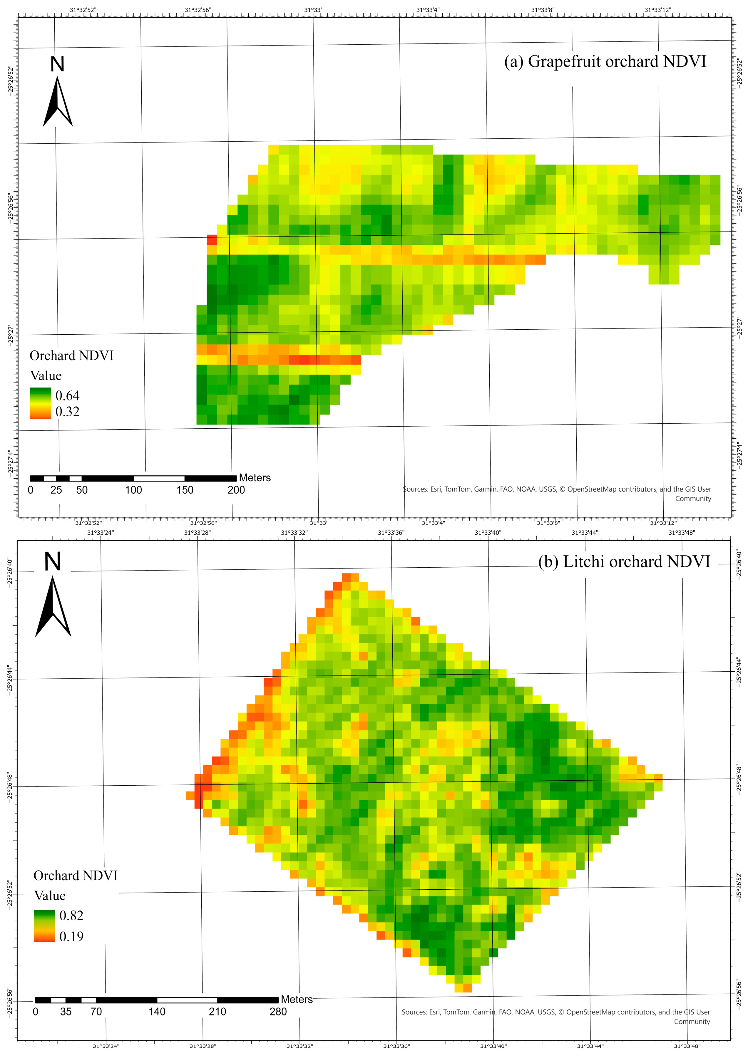
The orchard images were downloaded from the Sentinel 2 satellite in Google Earth Engine (GEE), and to minimize the influence of cloud cover, images with more than 20% cloud cover were filtered out. The orchard N D V I for the grapefruit, litchi, and mango were developed in ArcGIS Pro (ESRI, Redlands, CA, USA) using Equation (1):
N D V I = N I R R E D N I R + R E D
where N I R and R E D are the surface reflectance of the near infrared and red bands, respectively. The N I R and R E D corresponded to the bands B 8 and B 4 of the Sentinel 2 Multispectral Imager product [71].

2.2.3. Leaf Area Index

The orchards L A I ( m 2 of leaf area per m 2 ground area) were calculated using the normalized difference vegetation index ( N D V I ). The fractional vegetation cover was calculated using Equation (2) [72]:
F c = N D V I N D V I m i n N D V I m a x N D V I m i n
where F c is the factional vegetation cover, N D V I is the normalized difference vegetation cover, N D V I m i n is the minimum value of N D V I and N D V I m a x is the maximum value of N D V I . The N D V I m i n and N D V I m a x for the grapefruit, litchi and mango orchards were derived from the Sentinel 2 data (Table 2). N D V I m i n values of 0.32, 0.19, 0.30 were used for grapefruit, litchi, and mango, respectively, and values of 0.64, 0.82, 0.80 were used for grapefruit, litchi, and mango, respectively. The L A I for the orchards were calculated using Equation (3) [73,74]:
L A I = l n ( 1 F c ) k
where k is the extinction coefficient and a value of 0.5 was used in this study assuming leaf with random distribution [75].

2.2.4. Transpiration Measurements

The grapefruit, litchi, and mango tree transpiration was measured hourly over two growing seasons using the heat ratio method (HRM) [76] sap flow technique. In each orchard, a survey was conducted by measuring 25 randomly selected trees to establish the stem size distribution. Four trees representative of the stem size distribution from the smallest stem size to the largest per each orchard were instrumented with the HRM sap flow sensors (Andrew Everson, Pietermaritzburg, South Africa). A metal drilling guide with three holes positioned 0.5 cm apart was used to drill 0.2 cm diameter holes in the tree stems, reducing errors due to probe misalignment [69,77]. For each instrumented tree, four sets of T-type thermocouples were installed at depths of 1, 2, 3, and 4 cm, respectively, below the bark in the cardinal directions (north, south, east, and west directions), around the stem. This arrangement enabled the sap flow system to effectively track changes in the radial sap velocity of the stem [78,79]. Each pair of T-type thermocouples was installed upstream and downstream of a central heater probe, which was housed inside a brass sleeve to ensure even heat conduction. These thermocouples were then connected to the tree boxes. The HRM sap flow system in each orchard comprises four tree boxes, each assigned to a single instrumented tree. The tree box was equipped with four pairs of T-type thermocouples, four heaters, and control electronics. The tree boxes were connected to the CR1000 datalogger (Campbell Scientific, Logan, UT, USA) via the AM16/32B multiplexer (Campbell Scientific, Logan, UT, USA). The AM16/32B was used to expand the number of measuring channels for the thermocouples connected to the tree boxes. The CR1000 data logger was programmed to control the HRM sap flow system heat pulsing, read the thermocouples’ output, and store the hourly measurements. The HRM data were corrected for the trees’ wounding due to drilling and probe insertion using the approach proposed by Swanson and Whitfield [80]. The sapwood area for the litchi was determined by visually inspecting changes in the colour of wood from a slice that was cut from the tree stem. The sapwood area for the grapefruit and mango was determined by injecting a weak solution of methylene blue dye into the tree stems, followed by using a stem corer to collect a sample of stained wood above the dye injection points after three days. Individual tree sap flow volume (L/tree/h) was computed as a weighted sum of the products of the corrected tree sap velocity represented by each thermocouple probe and the sapwood area allocated to the respective probe. The transpiration for the orchards (mm/h) was computed from the hourly total weighted sap flow volume, considering the number of trees per hectare in each stem diameter class divided by the area of one hectare [28,69,77,81].

2.2.5. Evapotranspiration Measurements

The orchards’ actual evapotranspiration was measured on selected periods (Table 3) using an open-path eddy covariance system, which was mounted on a 10 m lattice mast and stationed at the centre of the orchard. The eddy covariance system was installed in the orchards for short window periods, lasting a few weeks (Table 3), owing to equipment shortages. The eddy covariance system comprised of an IRGASON (Campbell Scientific, Logan, UT, USA), EC100 (Campbell Scientific, Logan, UT, USA), CR3000 datalogger (Campbell Scientific, Logan, UT, USA), net radiometer (Model: NR-LITE2, Kipp & Zonen, Delft, The Netherlands), soil heat flux plates (Model: HFP01, Hukseflux, Delft, The Netherlands), averaging soil thermocouple probe (Model: TCAV, Campbell Scientific, USA), soil moisture sensors (Model: CS616, Campbell Scientific, Logan, UT, USA), temperature and relative humidity sensor (Model: EE181, Campbell Scientific, Logan, UT, USA). The IRGASON combined a three-dimensional sonic anemometer for measuring wind speed in the three axes (x, y, and z directions) and an infrared gas analyser (IRGA) for measuring the water vapour and carbon dioxide. The IRGASON was installed at a height of approximately 1.5 m above the tree canopies, facing in the direction of the prevailing wind. Measured data from the IRGASON were collected through the EC100 and then stored every 30 min into a CR3000 datalogger. The high-frequency data measured at 10 Hz were stored onto a 2 GB secure digital (SD) memory card connected to the CR3000 datalogger. The orchard net radiation was measured using an NR-LITE2 sensor, and this was mounted approximately 9.6 m above the orchard on a metal pole extension facing the northern direction to minimize shading effects. Soil heat flux was measured using 2 HFP01 sensors, which were installed at a depth of about 16 cm below the soil surface. Soil moisture content was measured using two CS616 sensors, and these were installed at a depth of about 8 cm below the soil surface. TCAV probes were installed at depths of 0.5, 5.5, 10.5, and 15.5 cm below the soil surface. The eddy covariance system used the EasyFlux DL CR3000OP software, version 1.2 (Campbell Scientific, USA) to collect and correct the output for carbon dioxide, latent heat, and sensible heat fluxes. The correction procedures included de-spiking, coordinate rotations, frequency corrections, among others [21].

2.3. Models’ Description

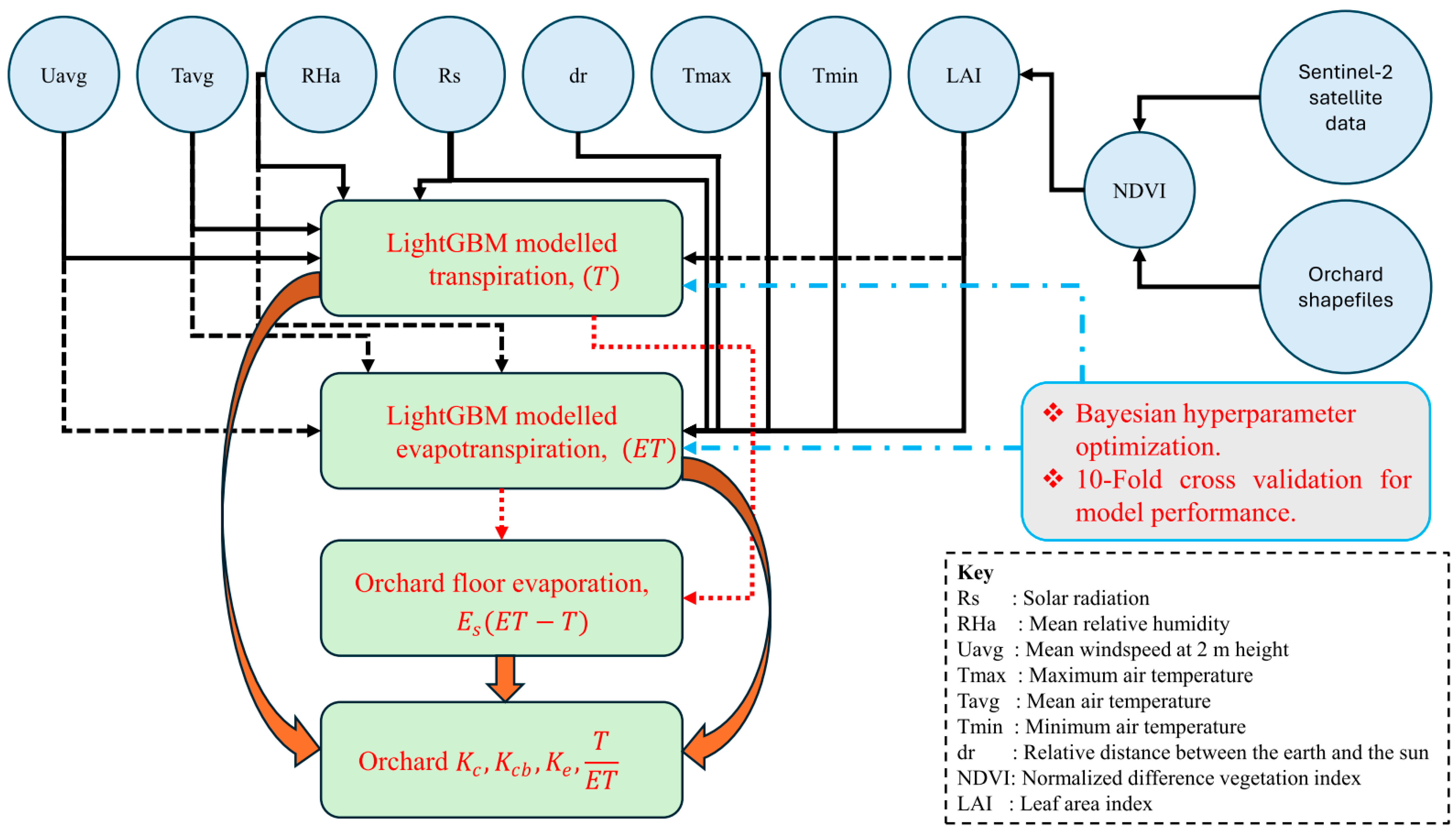
We proposed machine learning models for estimating evapotranspiration and transpiration based on the LightGBM model (Figure 2). In this current study, canopy interception ( I c ) was assumed to be lost via evaporation. Thus, the total orchard evaporation ( E s ) was taken as the sum of soil evaporation, I c and transpiration from understorey vegetation. Therefore, E s was calculated as the difference between the modelled orchard evapotranspiration and tree transpiration ( E T T ). The set of input variables for the machine learning models (Figure 2) was selected because it represented key parameters in the evapotranspiration and transpiration mechanisms.
The hourly evapotranspiration and transpiration for the three crops were modelled using Equations (4) and (5), respectively,
E T ~ L i g h t G B M L A I , R s , T m i n , T a v g , T m a x , R H a , U a v g , d r
T ~ L i g h t G B M R s , L A I , T a v g , R H a , U a v g
where R s is the solar radiation, L A I is the mean monthly leaf area index, T m i n is minimum air temperature, T a v g is the mean air temperature, T m a x is maximum air temperature, R H a is the mean relative humidity, U a v g is the mean windspeed at 2 m height, and d r is the relative distance between the Earth and the Sun.
LightGBM is a gradient learning framework that grows decision trees by applying a novel method that promotes both performance and efficiency. The objective function in LightGBM is fundamental as it controls the model’s training operation by utilising the loss function and regularization. The objective function ( L ) , can be expressed as in Equation (6):
L = i = 1 n l y i , y ^ i + k = 1 N Ω f k
where l y i , y ^ i is the loss function, y ^ i is the prediction for instance i , Ω f k is the regularization term for the k -th tree f k , n is the number of instances, N is the number of trees, and y i is the actual value for the i -th observation [82,83]. LightGBM utilizes a leaf-wise growth approach that chooses the leaf with the maximum loss reduction, thereby producing quicker convergence and reduction in memory consumption [65,67]. Thus, efficiency, accuracy, interpretability, and easy application in Python were the principal reasons we selected LightGBM for evapotranspiration and transpiration modelling. In the current study, we used LightGBM https://lightgbm.readthedocs.io/en/stable/index.html (accessed 25 May 2025) from the Python (v 3.12.6) machine learning library; scikit-learn was used to construct the evapotranspiration and transpiration models in Pycharm Community Edition (version 2025.1).
Measured data for the evapotranspiration and transpiration were split into training and validation sets. The training data constituted 80% of the measured data and the remaining 20% was reserved for model validation. To ensure model robustness and precise predictions, Bayesian hyperparameter optimization [84,85,86,87] was conducted on the models within the training datasets. This was performed by utilizing the Optuna hyperparameter optimization framework https://optuna.org/#key_features (accessed 25 May 2025) in the scikit-learn machine learning library.

2.4. Models’ Validation and Evaluation Metrics

2.4.1. Cross-Validation and Independent Validation

We adopted the k-fold (k = 10) cross-validation to randomly evaluate the overall LightGBM model performance using 80% of the measured data. In k-fold cross-validation, training data are grouped into k groups, then one group is reserved for testing, whilst the rest of the remaining groups are used for training the model. The procedure is repeated multiple times until all the groups have been applied as testing data [88]. An independent validation was performed on the developed LightGBM models using 20% of the measured data to assess the model’s performance on unseen data.

2.4.2. Validation Metrics

To evaluate the machine learning models against the orchards’ in situ measurements, the following metrics were adopted: coefficient of determination, R 2 [89], root mean square error, R M S E [90,91], mean absolute error, M A E [92], and Kling–Gupta efficiency, K G E [93,94]. The R 2 range from 0 to 1, with a value of 1 showing a perfect relationship between the actual and predicted data. A value of 0 reflects the absence of statistical correlation between the actual and predicted data [95]. The model prediction accuracy increases when R M S E approaches 0 [96]. The M A E range from 0 to infinity (∞), where a value of 0 indicates a perfect relationship between the actual and predicted data [97]. The K G E range from ∞ to 1, with a value of 1 showing a perfect relationship between actual and predicted data [98].

2.4.3. LightGBM Model Interpretability Analysis

The LightGBM model is too complicated to be explained directly [99]; thus, we used the SHAP (Shapley Additive exPlanations) summary plots to investigate the relative importance of the models’ input features and establish how these influenced the predicted output [45,100]. SHAP values are built based on the cooperative game theory [101,102,103], and these are used to rank model input features, where features possessing greater SHAP values are considered more dominant [82]. The SHAP value for the model input feature i is calculated using Equation (7) [45,100]:
ϕ i = S N i S ! N S 1 ! N ! k S i k S
where ϕ i is the SHAP value for feature i , S is a subset of features excluding i , N is the set of all the features, and k ( S ) is the value function for the subset S .

3. Results

3.1. Microclimate

A monthly summary of the weather conditions and orchard leaf area indices during the 2021/23 growing seasons is shown in Table 4. The study area received rain almost throughout the year, with most rain concentrated in the summer seasons (November–March). Over the entire 24 months of the study, average solar radiation peaked in the summer seasons, producing approximately 21.0 MJ/m2/d in February 2022, while an average minimum value of 11.60 MJ/m2/d was observed in May 2023. Daily maximum air temperature reached 43.0 °C in October 2022, and a daily minimum air temperature of 7 °C was observed in June 2022. The average relative humidity was above 60% throughout the study period, peaking in the summer months. Wind speed at the study site changed slightly between months, with the average values ranging between 1.01 and 1.53 m/s. The total reference evapotranspiration ( E T o ) peaked in the summer season, with a maximum value of about 155 mm/month recorded in January 2023, and reached a minimum in the winter months, recording a minimum of 71 mm/month in June 2022. The trend suggested that the water use of the trees (grapefruit, litchi and mango) would be lower in the winter season as compared to the summer season, owing to low atmospheric evaporative demand. The total rainfall and E T o for the study period were approximately 1668 mm and 2664 mm, respectively.

3.2. Orchard Leaf Area Index ( L A I )

The Sentinel 2-derived N D V I was used to calculate the monthly average orchard L A I over the course of the 2-year study period (Table 4). A summary of the grapefruit, litchi and mango orchard maximum N D V I , minimum N D V I , mean N D V I and N D V I standard deviation is shown in Table 2. The spatial N D V I for the grapefruit, litchi, and mango orchards computed from the Sentinel 2 data are shown in Figure 3a–c. Monthly average orchard L A I ranged between 1.53 and 4.32 for grapefruit, 2.10 and 5.33 for litchi, 2.02 and 4.68 for mango, respectively. The monthly Sentinel 2 L A I was used to model both the orchard evapotranspiration and tree transpiration.

3.3. Transpiration and Evapotranspiration Models Accuracy

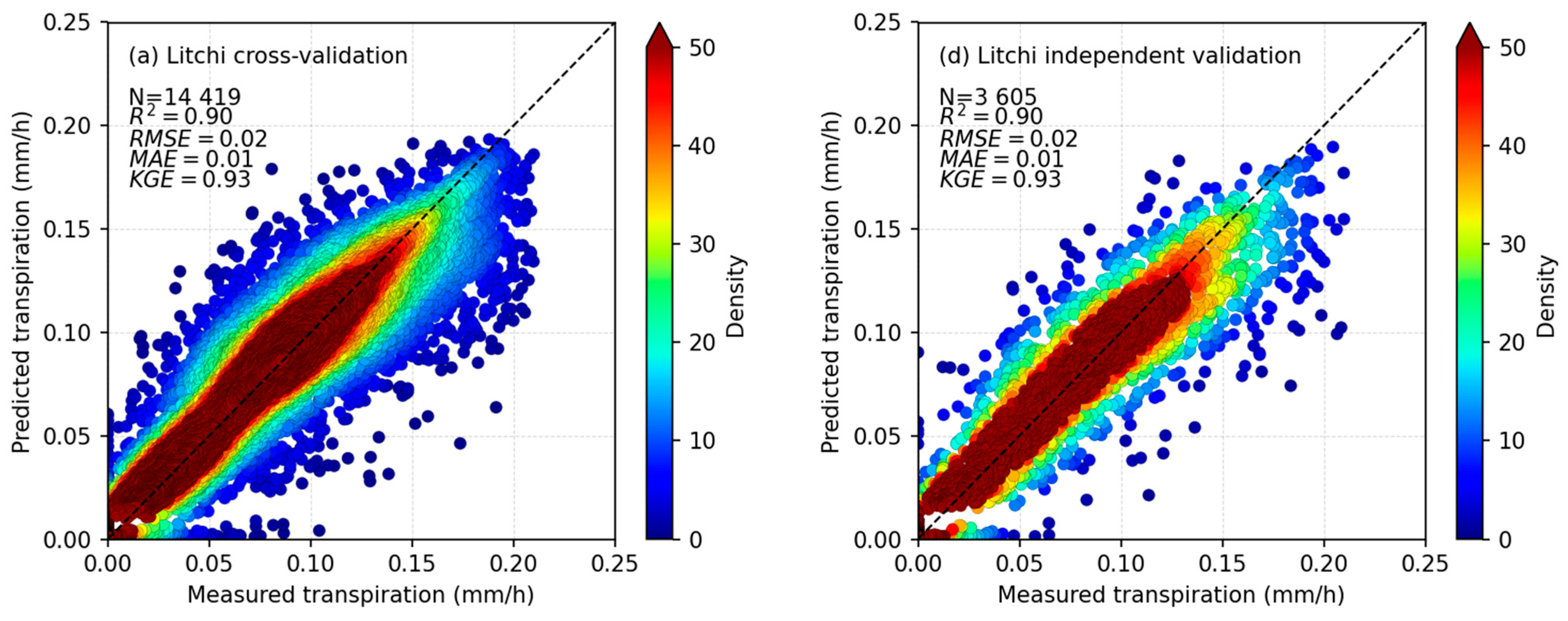
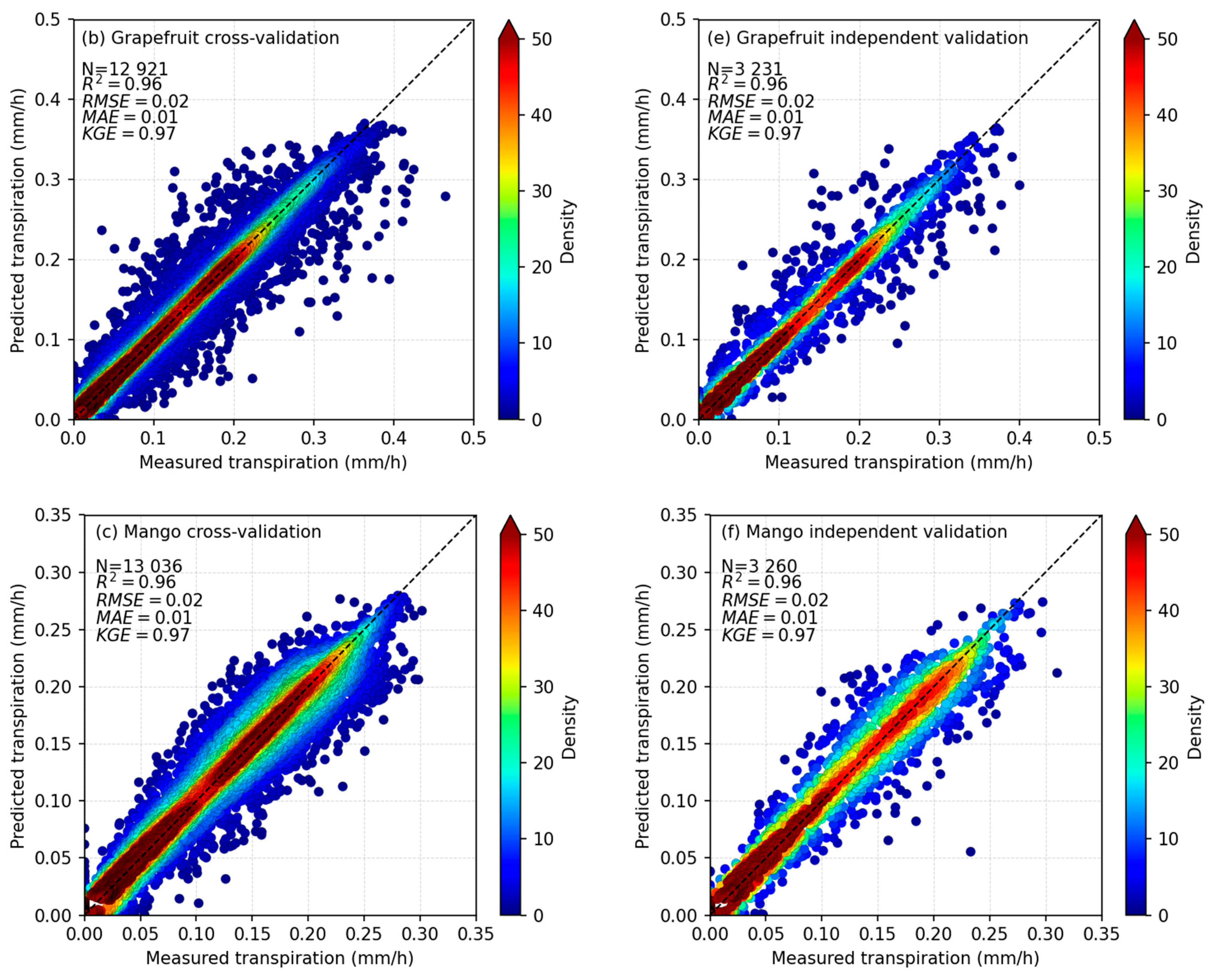
Transpiration and evapotranspiration for litchi, grapefruit, and mango were modelled using the LightGBM learning models and input parameters shown in Figure 2. A comprehensive evaluation of the applied LightGBM transpiration and evapotranspiration models was implemented using graphical plots and statistical metrics. Six LightGBM models were trained using T and E T training datasets for the three crops (litchi, grapefruit, mango), and Bayesian hyperparameter optimization was used to search for the models’ optimal parameter configurations. The optimal parameters obtained for the evapotranspiration and transpiration LightGBM models are shown in Table 5. The scatter plots shown in Figure 4 and Figure 5 express the relationship between actual and modelled values for the training and validation datasets.
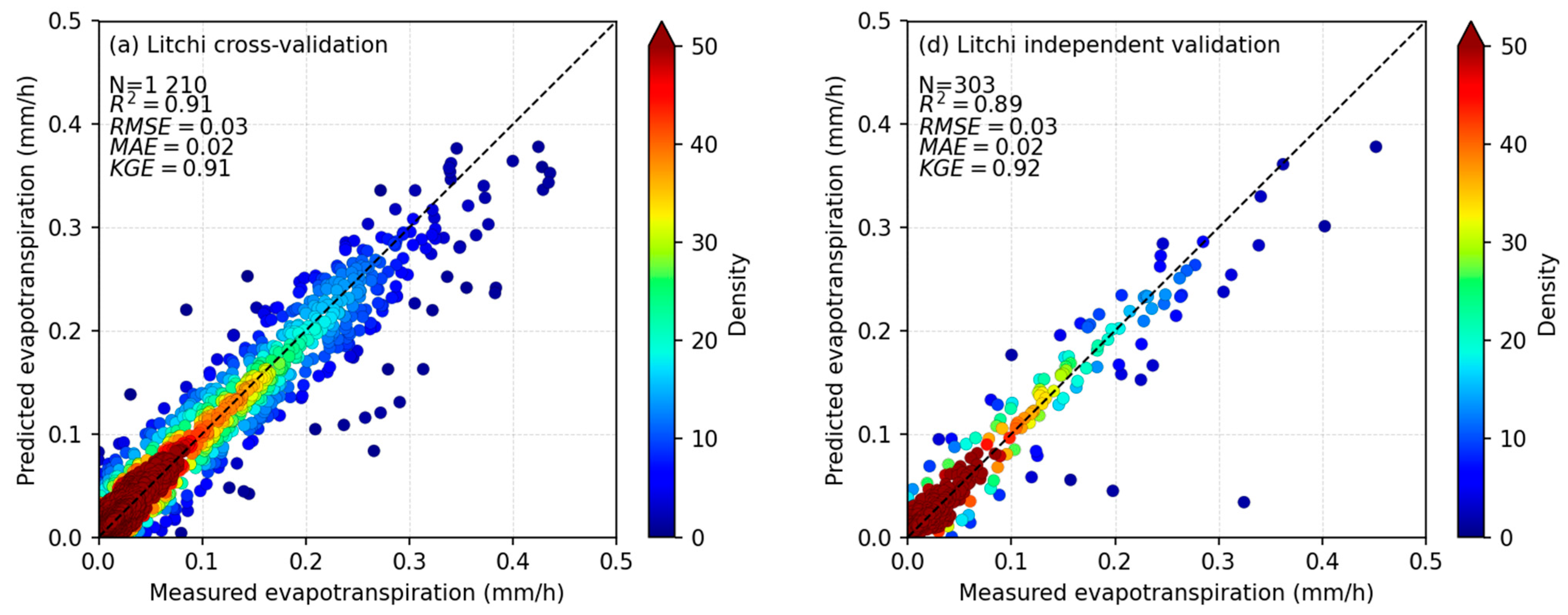
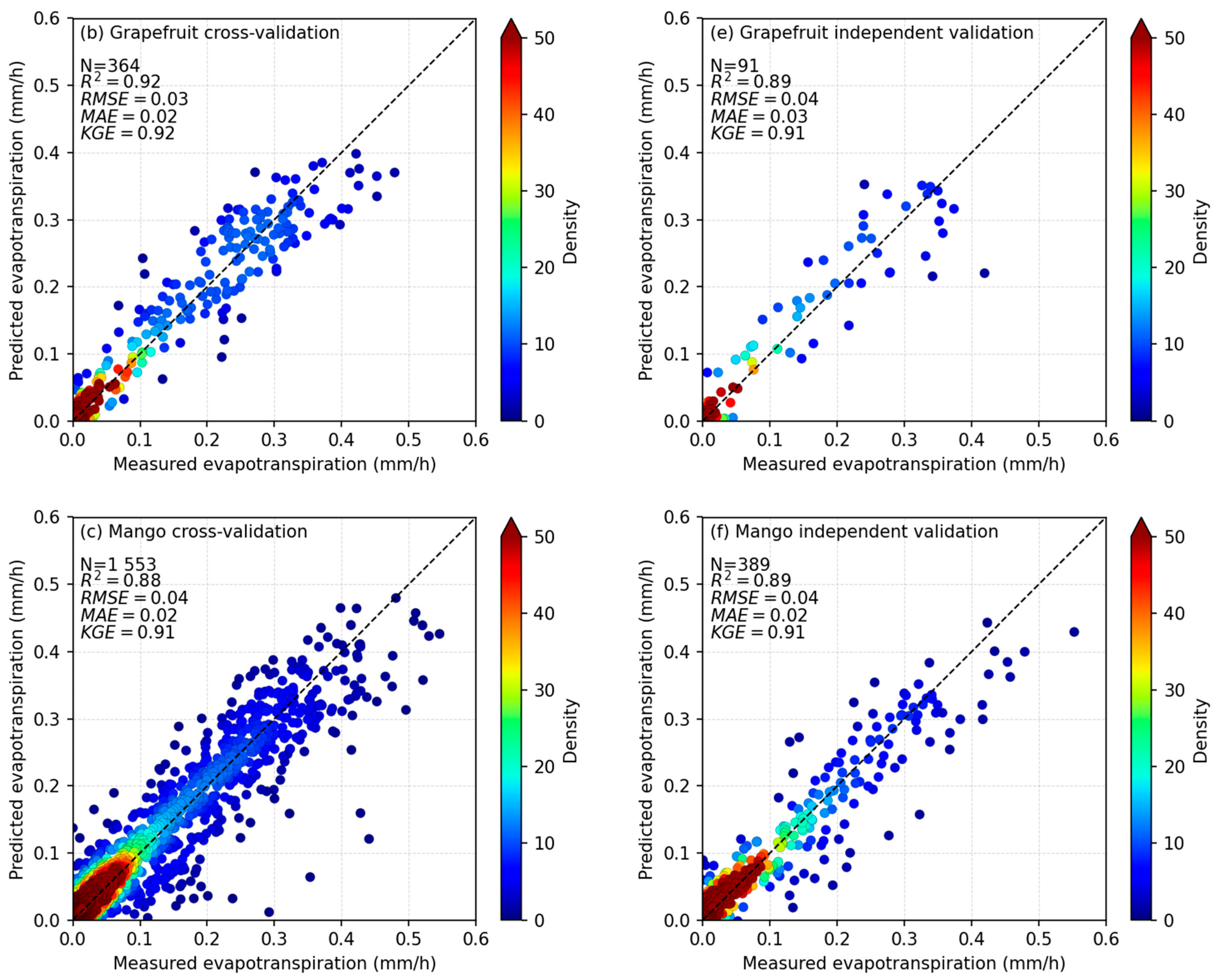
To assess the robustness of the T and E T models, we performed 10-fold cross-validation on the training datasets for the three crops. In the 10-fold cross-validation, the training datasets were divided into ten subsets, where at each moment the models were trained using nine subsets while the remaining one was used for testing. The process was repeated 10 times until all the subsets had been used as the testing data. The performance of the models was evaluated by calculating the R 2 , R M S E , M A E and K G E evaluation metrics of each of the 10 test subsets. Ultimately, an average was computed for each evaluation metric to give a more reliable estimate of the models’ performance. The cross-validation for the transpiration models produced acceptable results with a minimum R 2 of 0.90, R M S E = 0.02 mm/h, M A E = 0.01 mm/h, minimum K G E of 0.93 (Figure 4a–c) and the evapotranspiration models produced acceptable results with a minimum R 2 of 0.88, maximum R M S E of 0.04 mm/h, M A E = 0.02 mm/h and minimum K G E of 0.91 (Figure 5a–c). An independent validation was performed on the developed LightGBM models using the validation datasets to assess the model’s performance on unseen data. There was a consistent performance of the models on the validation datasets for the three crops as reflected by the transpiration models producing a minimum R 2 of 0.90, R M S E = 0.02 mm/h, M A E = 0.01 mm/h, minimum K G E of 0.93 (Figure 4d–f). The evapotranspiration models produced an R 2 of 0.89, maximum R M S E of 0.04 mm/h, maximum M A E of 0.03 mm/h, and minimum K G E of 0.91 (Figure 5d–f). The actual and modelled data for all the transpiration and evapotranspiration LightGBM learning models demonstrated strong relationships, converging near the lines of best fit (1:1 lines). Thus, the results from the cross-validation and independent validation reflected that these LightGBM learning models were stable and robust, hence have the potential to model transpiration and evapotranspiration for the three crops. Furthermore, post-processing investigations were conducted to gain a deeper understanding of the models.

3.4. LightGBM Learning Model Interpretability

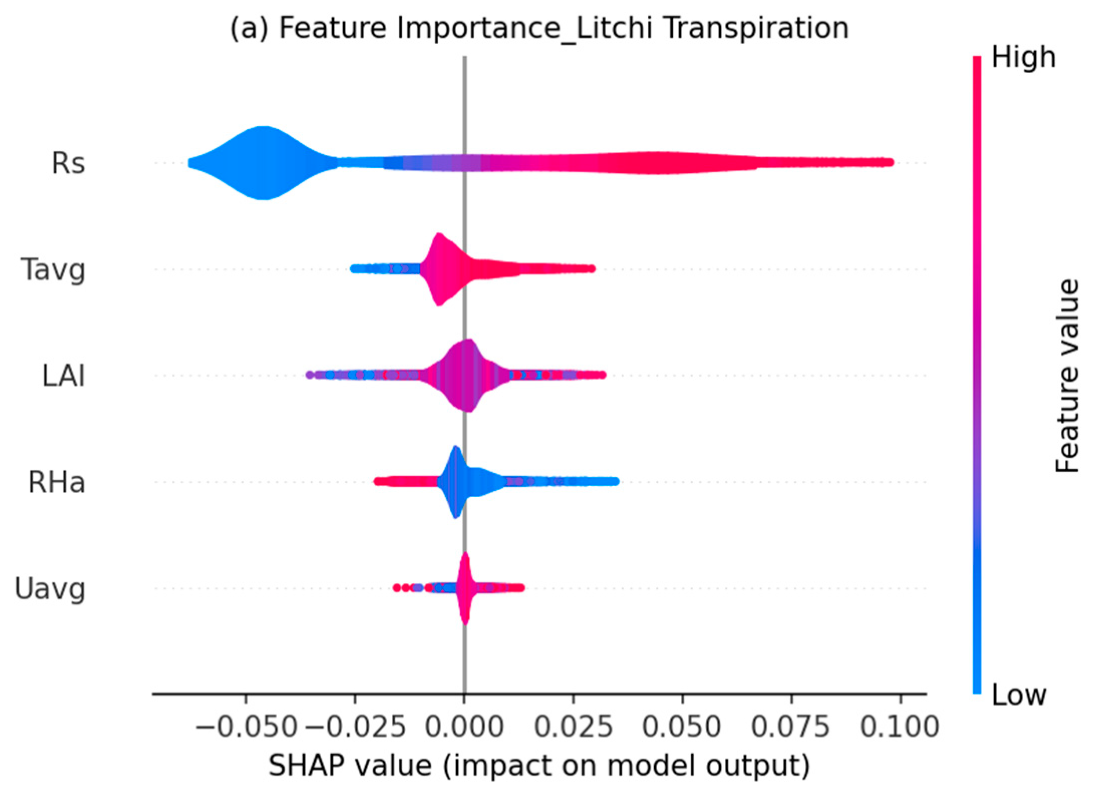
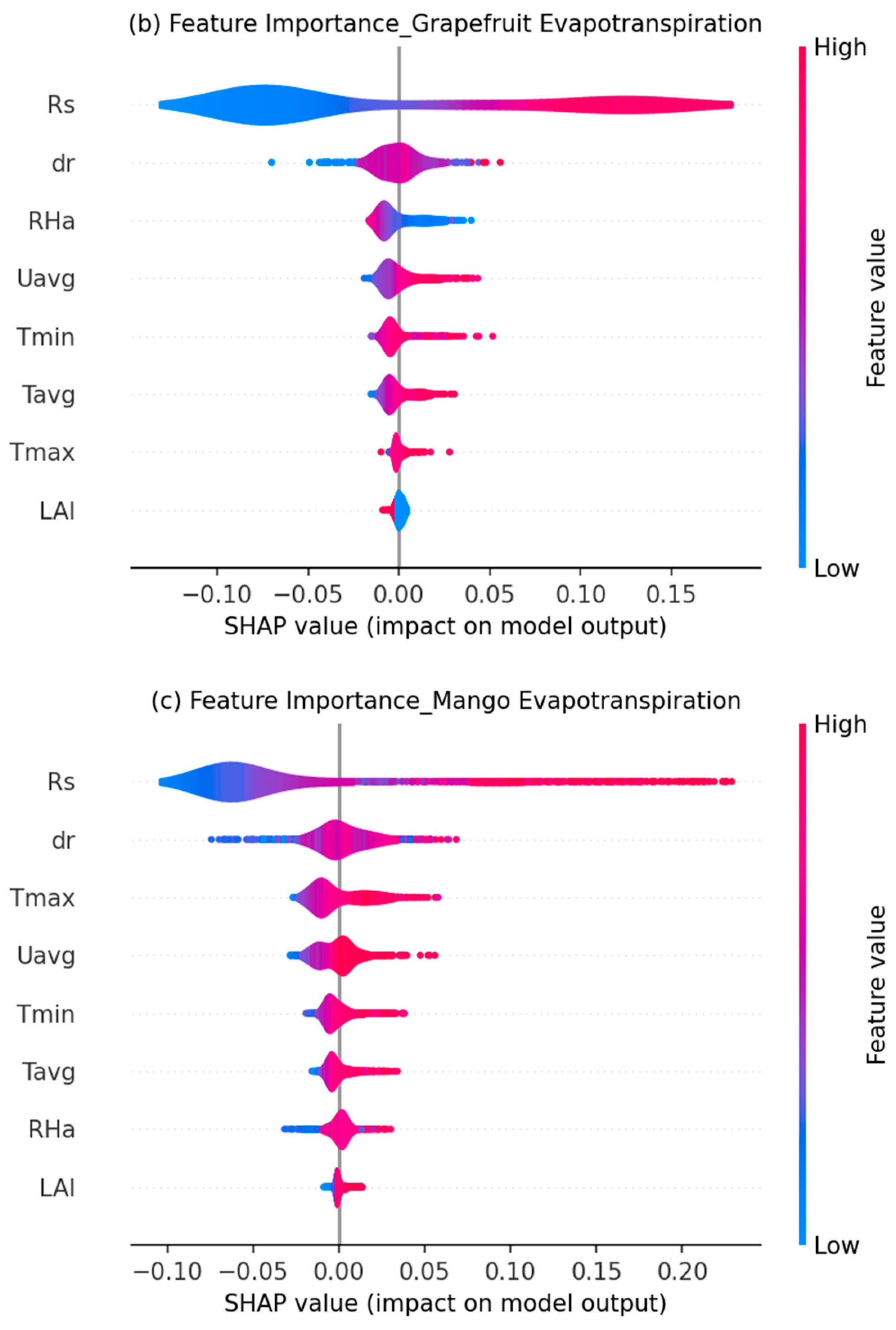
In this study, we utilized the SHAP summary plots to investigate the significance of predictor variables and ascertain their effect on the transpiration and evapotranspiration modelled output. The size of the SHAP value is displayed on the horizontal axis (x-axis), and its magnitude indicates either a positive or negative influence on the modelled output. The distribution of SHAP values for each predictor variable in forecasting transpiration and evapotranspiration for the three crops is shown in Figure 6 and Figure 7. Among the five input predictor variables for the transpiration model, R s indicated the highest impact on the modelled transpiration for the three crops, followed by T a v g , L A I , R H a and U a v g , respectively (Figure 6a–c). The R s and T a v g exhibited a positive correlation with the modelled transpiration, while R H a indicated a negative correlation with the modelled transpiration.
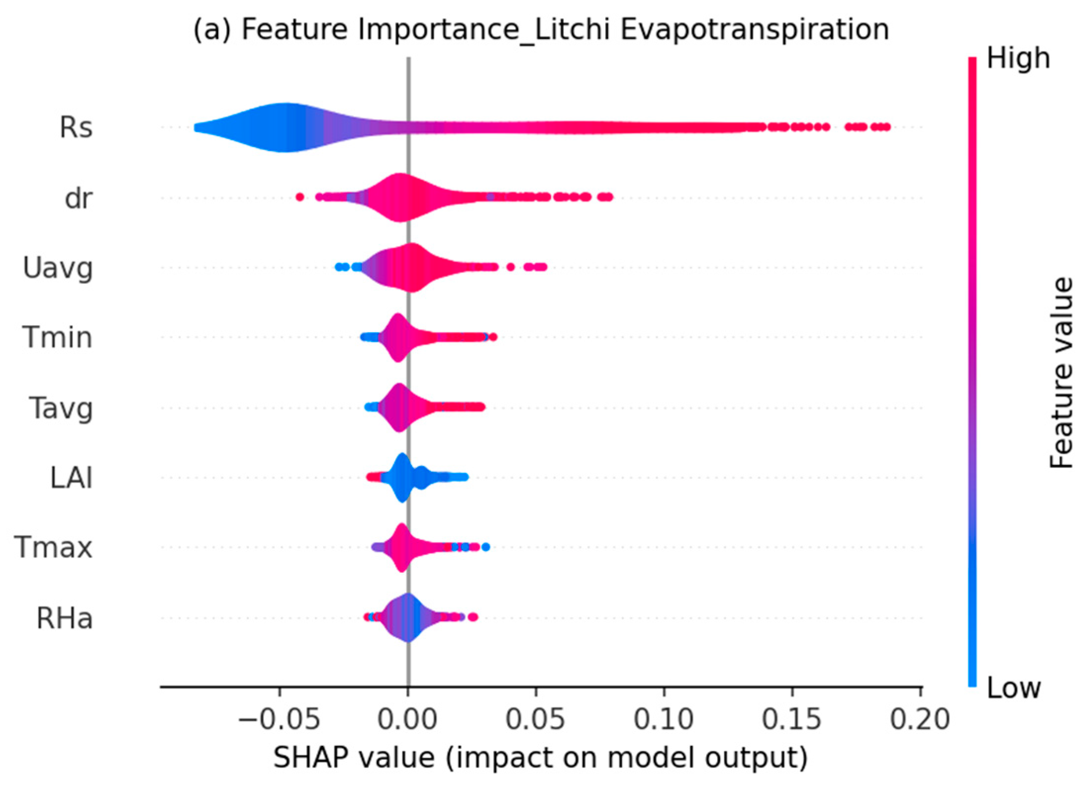
The R s had the largest influence on the litchi evapotranspiration model, followed by d r , U a v g , T m i n , T a v g , L A I , T m a x , and R H a , respectively (Figure 7a). For the grapefruit, R s showed the highest impact on the modelled evapotranspiration, followed by d r , R H a , U a v g , T m i n , T a v g , T m a x , and L A I , respectively (Figure 7b). Among the input predictors for the mango evapotranspiration model, R s exhibited the largest impact on the modelled evapotranspiration, followed by d r , T m a x , U a v g , T m i n , T a v g , R H a and L A I , respectively (Figure 7c). The R s and d r exhibited the largest influence on all the evapotranspiration models for the three crops, and R s , U a v g , T m i n , T a v g indicated a positive correlation with the modelled evapotranspiration (Figure 7a–c).

3.5. Orchard Evapotranspiration Partitioning Dynamics

3.5.1. Orchard E T , T and E s

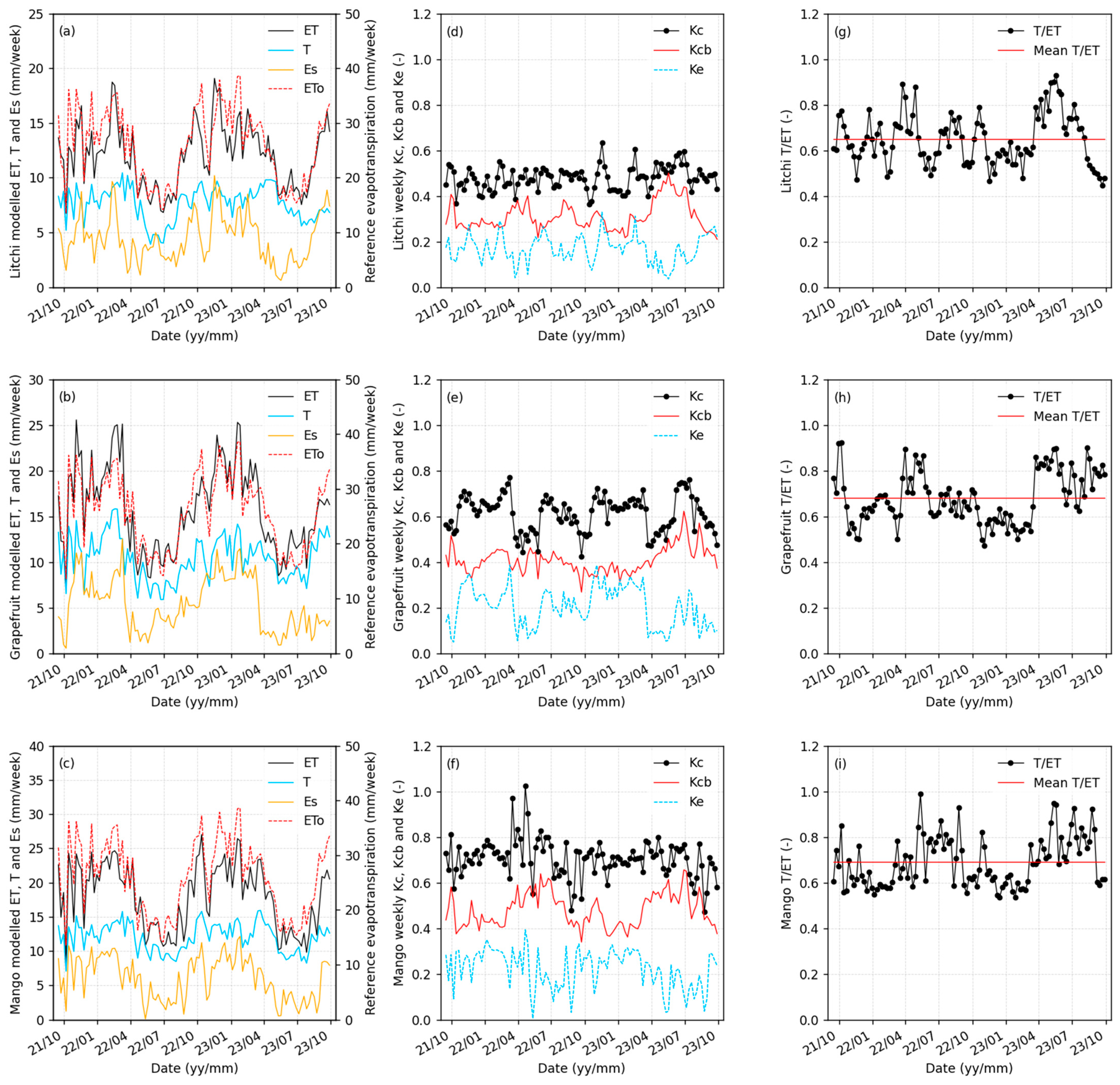
The litchi, grapefruit and mango E T , T , and E s showed maximum weekly total value in the summer season (November–March) and a minimum value in the winter season (May–July), except in October 2021 where a decrease was observed in E T , T , E s as shown in Figure 8a–c. The decrease in E T , T , E s was attributed to the sharp decrease in E T o , which caused a reduction in the atmospheric evaporative demand. The E T , T , and E s for the three crops followed the same seasonal trend as the E T o . Maximum T for litchi, grapefruit and mango occurred in the summer season, giving cumulative totals of 10.5 mm/week, 15.8 mm/week, 16.0 mm/week, respectively, and minimum T was recorded in the winter season with values of 4.0 mm/week, 5.9 mm/week and 7.0 mm/week, respectively. The annual average modelled transpiration for litchi, grapefruit, and mango was approximately 397 mm, 541 mm, and 624 mm, respectively.
The orchard E s comprised a combination of soil evaporation, I c and transpiration from periodic understorey vegetation. The minimum orchard E s for the litchi, grapefruit, mango was recorded in the winter season, giving values of 0.6 mm/week, 0.9 mm/week and 0.1 mm/week, respectively. The maximum orchard E s for the litchi, grapefruit and mango was recorded in the summer season, giving values of 10.2 mm/week, 12.5 mm/week and 12.1 mm/week, respectively. The annual average orchard E s for litchi, grapefruit and mango was approximately 230 mm, 281 mm and 313 mm, respectively.
The maximum E T for litchi, grapefruit and mango occurred in the summer season, giving values of 19.1 mm/week, 25.6 mm/week and 27.0 mm/week, respectively. The corresponding minimum E T was recorded in the winter season with values of 6.7 mm/week, 7.1 mm/week and 8.3 mm/week, respectively. The annual average modelled E T for litchi, grapefruit and mango was about 626 mm, 823 mm, and 937 mm, respectively. Mango had the largest cumulative E T , T , and E s , followed by grapefruit and litchi.

3.5.2. Crop Coefficient, Basal Coefficient, and Soil-Evaporation Coefficient

The derived weekly crop coefficient ( K c ), weekly basal crop coefficient ( K c b ), weekly orchard evaporation coefficient ( K e ) for litchi, grapefruit, and mango are shown in Figure 8d–f. The K c was computed by dividing the modelled E T with E T o . The K c b was calculated by dividing the modelled T with E T o . Orchard floor evaporation coefficient ( K e ) was calculated by dividing the total orchard evaporation (sum of soil evaporation, I c and understorey vegetation transpiration) with E T o . The litchi orchard K c , K c b and K e varied throughout the study period. There was a marked increase in K c b between January 2023 and October 2023, which coincided with the litchi tree flowering to postharvest period. The litchi K c ranged between 0.36 and 0.64, K c b ranged between 0.21 and 0.50, and K e ranged between 0.04 and 0.33 for the duration of the study (Figure 8d). There was a marked decrease in the grapefruit orchard K c and K e in the winter seasons. This coincided with the orchard understorey spraying, mowing, and a decrease in rainfall, which we attribute to the decrease in the orchard evaporation. Grapefruit K c ranged between 0.61 and 0.77, K c b ranged between 0.41 and 0.62, and K e ranged between 0.05 and 0.39 (Figure 8e). The K c for mango varied throughout the study period. There was an increase in mango K c b between January and October, which represented the mango four-stage crop coefficients. The mango K c varied between 0.71 and 1.02, K c b varied between 0.34 and 0.66, and K e varied between 0.005 and 0.39, respectively (Figure 8f).

3.5.3. E T Partitioning

The derived weekly ratios of tree transpiration to orchard evapotranspiration T E T for litchi, grapefruit and mango are shown in Figure 8g–i. The ratio T E T was determined by dividing the orchard evapotranspiration into productive plant transpiration and non-productive orchard floor evaporation. The ratio E s E T was determined by subtracting T E T from unity. The litchi T E T varied throughout the study, ranging between 0.45 and 0.93, with an overall mean value of 0.65 (Figure 8g). The average litchi E s E T ranged between 0.55 and 0.07 during the same period, giving a mean value of 0.35. The grapefruit T E T ranged between 0.47 and 0.92 for the study duration, giving an average value of 0.68 (Figure 8h). The calculated grapefruit E s E T over the same period ranged between 0.53 and 0.08 with an average value of 0.32. Mango orchard T E T varied between 0.54 and 0.99, producing an average value of 0.69 (Figure 8i). Over the same period, mango orchard E s E T varied between 0.46 and 0.01, producing an overall average of 0.31. The orchard T E T for the three crops recorded minimum values during the summer season and maximum values in the winter season, thereby producing maximum and minimum E s E T values in the summer and winter seasons, respectively. This was attributed to the increase in the orchard evaporation during the summer season as compared to the winter season. The increase in orchard evaporation was due to constant rainfall, orchard floor wetting, and sizable presence of understorey vegetation.

4. Discussion

Accurate estimation of actual E T and its partitioning into productive crop transpiration and non-productive orchard floor losses is very essential in the precise design and planning of irrigation schedules for orchards [4,6,38,104,105,106]. Actual E T and T modelling using machine learning models have gained popularity over the past few years due to their exceptional capabilities of solving complex non-linear relationships between predictor and target variables [107].
The accuracy of the E T and T models reported for litchi, grapefruit, and mango orchards in the current study indicated R 2   0.88, K G E   0.91, R M S E   0.04 mm/h, and M A E   0.03 mm/h, respectively, having the same order of accuracy as those observed in other studies. For example, a study to measure E T of a site that mainly comprised of Bahia pastures grass was conducted in the subtropical humid climate of central Florida, United States of America. The E T measurements were carried out using an eddy covariance system over a period of 4 years, and this was used to model E T using M5P regression tree, bagging, random forests, and support vector regression models, respectively. The comparison between the measured and predicted E T produced an average Nash–Sutcliffe Efficiency ( N S E ) of 0.96, R M S E of 0.31 mm/d, M A E of 0.24 mm/d [108]. Daytime E T for Nissouri Creek, Ontario, Canada, was measured using a Bowen ratio energy balance system over a period of 4 months, and this was used to model E T using an artificial neural network model. The results between the measured and predicted E T produced an average R 2 of 0.99, R M S E of 0.59 mm/d, M A E of 0.38 mm/d [109]. The daily E T of green peppers was measured over a period of 5 years using the soil water balance method in the continental monsoon climate of Hebei province, China, and this was used to build the Elman neural network E T model. The results between the measured and predicted E T produced an average R 2 of 0.92, N S E of 0.91, R M S E of 0.48 mm/d, M A E of 0.4 mm/d [110]. The E T of a citrus orchard was measured over a period of 4 years using the eddy covariance system in the Mediterranean climate of Palermo, Italy and this was used to build the random forests and multi-layer perceptron E T models. The comparison between the measured and predicted E T produced an average R 2 of 0.77, R M S E of 0.48 mm/d [111]. The T of greenhouse potted tomato plants was measured over a period of 3 months using a real-time weighing system at the Agricultural University, China. The measured T was used to build random forests, back-propagation neural network, and genetic algorithms with back propagation neural network T models. The comparison between the measured and predicted T produced an average R 2 of 0.88 [60]. The LightGBM indicated good performance when compared to the tree-based M5 model tree, random forest, and four empirical models in daily reference evapotranspiration modelling for the subtropical region of China [67]. The E T of 16 cropland sites were measured using eddy covariance systems over a period of 20 years and this was partitioned using six machine learning models. The XGBoost produced the best results as compared to the artificial neural networks, extremely randomized trees, gradient boosting decision tree, LightGBM and random forest, with a correlation coefficient ( R ) of 0.88, R M S E of 6.87 W/m2, N S E of 0.77, M A E of 3.41 W/m2 [38]. The results demonstrated that the developed LightGBM learning models are suitable for predicting subtropical trees (litchi, grapefruit, and mango) E T and T .
Weekly maximum E T for litchi was approximately 19.1 mm/week, and this was lower than the value that was reported by Menzel et al. [112]. They reported a value of 26 mm/week for a study that was conducted on 10-year-old well-watered litchi trees in South Africa. The difference was attributed to the high range of evaporation from a Class A pan (20 mm/week–70 mm/week) which converted to E T o range of 15 mm/week–53 mm/week (using the pan coefficient value of 0.75) as compared to the E T o range of 14 mm/week–39 mm/week in the current study. Thus, high E T o causes large atmospheric evaporative demand, which leads to an increase in E T [113]. The annual average modelled E T for grapefruit in the current study was approximately 823 mm. This was higher than the annual E T values that were measured on a grapefruit orchard at Çukurova University Agricultural Farm and Adana in Turkey. The E T values were measured using Bowen ratio–energy balance and eddy-covariance methods, yielding values of 716.9 mm and 640.4 mm, respectively [114]. The low E T observed for grapefruit in Turkey was attributed to the low orchard planting density (156 trees/ha) as compared to our current study (476 trees/ha). The annual average mango E T in the current study was about 937 mm and this was consistent with the findings reported in other studies. For instance, Nel et al. [69] in South Africa reported annual mango orchard E T values of 1060 mm and 802 mm using the A&P method and dual-source model, respectively. The modelled E T using the A&P method and the dual-source model differed by approximately 14% of the LightGBM modelled E T in the current study. In another study on a 7-year-old mango orchard in San Francisco River Valley, Petrolina-PE, Brazil, E T values of 555 mm and 552 mm were obtained over a period of 6 months (June to November) using Bowen ratio–energy balance and soil water balance methods, respectively [115]. These estimates were in a similar range to our findings, because the study of de Azevedo et al. [115] reported results over a period of 6 months; thus, when projected to cover the whole year, that may closely resemble the modelled mango E T in the current study.
The litchi K c in the current study varied in the range of 0.36–0.64 without a clear seasonal trend (Figure 8d). The observed range was less than the range of 0.4–1.2 that was reported by Menzel et al. [112] in a study that was conducted on a 10-year-old ‘Mauritius’ litchi orchard in Nelspruit, South Africa. However, they reported a lack of litchi K c seasonal trend [112], which was consistent with our results. The grapefruit K c determined in the current study ranged between 0.61 and 0.77 (Figure 8e). The derived K c values range was greater than the range 0.58–0.64 that was reported for a citrus crop in the semi-arid Souss-Massa region of Morroco [116]. The mango K c values varied in the range 0.71–1.02, which closely matched one of the K c ranges that were reported for high-density mango orchards [117]. The results indicate that the crop K c values are variable between regions owing to the differences in the climate, soils, management practices, among others. Thus, determination of representative crop coefficients under local conditions is necessary [118,119].
The average annual E s E T ratio for litchi, grapefruit and mango orchards in the current study was 0.35, 0.32, and 0.31, respectively (Figure 8g–i). The litchi orchard had the largest E s E T ratio, as compared to the grapefruit and mango orchards. This was attributed to the low planting density in the litchi orchard (70 trees/ha) which created large tree interrow spacings as compared to the grapefruit (476 trees/ha) and mango (303 trees/ha) orchards. Hence, the litchi orchard floor received a considerable amount of radiative energy, leading to an increased orchard floor evaporation [120] as compared to the grapefruit and mango. The findings in the current study are consistent with other evapotranspiration studies; for example, Kool et al. [4] reported 32 studies that derived E s E T ratios that exceeded 30%. Ntshidi et al. [121] reported an E s E T of 28% and 15% for micro sprinkler and drip irrigated commercial orchards in South Africa. The partition results indicated that orchard evaporative losses account for a significant portion of the orchard E T ; thus, more attention is needed to find sustainable ways of minimizing their contribution while promoting the productive water use ( T ).

5. Conclusions

The main objectives of the present study were to test the feasibility of using LightGBM learning to model T and E T for three crops (grapefruit, litchi, and mango) and use the derived data to partition the selected crops’ water use. In the current study, average monthly orchard L A I ranged between 1.60 and 4.32 for grapefruit, 2.10 and 5.33 for litchi, 2.02 and 4.68 for mango, respectively. Measured data for the evapotranspiration and transpiration were split into training and validation sets, in the ratio 80:20%. LightGBM from the Python (v 3.12.6) machine learning library scikit-learn was used to construct the evapotranspiration and transpiration models for the three crops. The models were optimized within the training datasets using Bayesian hyperparameter optimization to ensure robust and precise predictions. The 10-fold cross-validation was performed on the training datasets to test the model’s robustness, and an independent validation was performed on the validation datasets. The 10-fold cross-validation and independent validation on E T and T models produced a good accuracy with R 2   0.88, K G E   0.91, R M S E   0.04 mm/h, and M A E   0.03 mm/h for all the crops. SHAP analysis on the E T and T models for the three crops indicated that R s had the largest impact on the modelled E T and T among all the input predictor variables. The modelled E T , T , and E s for the litchi, grapefruit and mango followed the same seasonal trend as the E T o . Maximum and minimum E T , T , and E s for litchi, grapefruit and mango occurred in the summer and winter seasons, respectively. Annual average modelled transpiration for litchi, grapefruit, mango was approximately 397 mm, 541 mm, and 624 mm, respectively. The annual average orchard E s for litchi, grapefruit and mango was approximately 230 mm, 281 mm and 313 mm, respectively. The annual average modelled E T for litchi, grapefruit and mango was about 626 mm, 823 mm, and 937 mm, respectively. The litchi, grapefruit and mango K c values ranged between 0.36 and 0.64, 0.61 and 0.77, 0.71 and 1.02, respectively. The annual average E s E T ratio for litchi, grapefruit and mango orchards was 0.35, 0.32, and 0.31, respectively, with the litchi orchard having the largest E s E T ratio, followed by the grapefruit and mango orchards. The study demonstrates that the LightGBM model can accurately model the transpiration and evapotranspiration for subtropical crops using weather data, L A I , and d r . The orchard evaporation contributes a significant portion to the total orchard evapotranspiration, thus further improvements on orchard management practices can be utilized to minimize the orchard evaporative losses while promoting the productive water use ( T ).
This study was conducted on a single study site, and the actual E T for the litchi, grapefruit and mango orchards were measured over shorter periods owing to equipment shortages. This caused a limitation to the study, as we were not able to measure the complete E T seasonal trends for the three crops. This led to a limited training dataset for the E T models’ development and could result in the developed models being site-specific. Subsequently, regarding the derived K c values and the partitioning ratios, while applicable to this current study, care must be taken when attempting to apply these values in other locations. Therefore, extensive validation is recommended for the derived models on independent data from other subtropical crop orchards in other regions.

Author Contributions

Conceptualization, P.D., Z.E.M. and S.D.; methodology, P.D., Z.E.M. and S.D.; software, P.D.; validation, Z.E.M., P.J.R.C. and S.D.; formal analysis, P.D.; investigation, P.D., J.N.M., S.G., Z.N. and V.N.; resources, Z.E.M., P.J.R.C., T.S. and S.D.; data curation, P.D.; writing—original draft preparation, P.D.; writing—review and editing, Z.E.M., P.J.R.C., J.N.M., S.G., Z.N., V.N., T.S. and S.D.; visualization, P.D., Z.E.M., Z.N. and S.G.; supervision, Z.E.M., P.J.R.C. and S.D.; project administration, S.D.; funding acquisition, Z.E.M., T.S. and S.D. All authors have read and agreed to the published version of the manuscript.

Funding

This research was funded by Water Research Commission (WRC) and the Inkomati-Usuthu Catchment Management Agency in South Africa, Project WRC C2020/2023-00399.

Data Availability Statement

The data presented in this study are available upon request from the corresponding author.

Acknowledgments

The research reported here formed part of a bigger project entitled: “Developing a decision support system for estimating the water use and efficiency of irrigated crops in the Inkomati-Usuthu Water Management Area (WMA)”-Water Research Commission-Project WRC C2020/2023-00399. We acknowledge and express our gratitude to the Water Research Commission (WRC) and the Inkomati-Usuthu Catchment Management Agency in South Africa for funding and managing the project. We also thank Riverside Farm for allowing us to work in their productive orchards. We gratefully acknowledge the farm manager Dean van Heerden, for all the assistance.

Conflicts of Interest

The authors declare no conflicts of interest.

References

  1. Li, Y.; Liu, X.; Zhang, X.; Gu, X.; Yu, L.; Cai, H.; Peng, X. Using Solar-Induced Chlorophyll Fluorescence to Predict Winter Wheat Actual Evapotranspiration through Machine Learning and Deep Learning Methods. Agric. Water Manag. 2025, 309, 109322. [Google Scholar] [CrossRef]
  2. Tabari, H.; Kisi, O.; Ezani, A.; Hosseinzadeh Talaee, P. SVM, ANFIS, Regression and Climate Based Models for Reference Evapotranspiration Modeling Using Limited Climatic Data in a Semi-Arid Highland Environment. J. Hydrol. 2012, 444–445, 78–89. [Google Scholar] [CrossRef]
  3. Aytek, A. Co-Active Neurofuzzy Inference System for Evapotranspiration Modeling. Soft Comput. 2009, 13, 691–700. [Google Scholar] [CrossRef]
  4. Kool, D.; Agam, N.; Lazarovitch, N.; Heitman, J.L.; Sauer, T.J.; Ben-Gal, A. A Review of Approaches for Evapotranspiration Partitioning. Agric. For. Meteorol. 2014, 184, 56–70. [Google Scholar] [CrossRef]
  5. Shukla, S.; Jaber, F.H.; Goswami, D.; Srivastava, S. Evapotranspiration Losses for Pepper under Plastic Mulch and Shallow Water Table Conditions. Irrig. Sci. 2013, 31, 523–536. [Google Scholar] [CrossRef]
  6. Achite, M.; Jehanzaib, M.; Sattari, M.T.; Toubal, A.K.; Elshaboury, N.; Wałęga, A.; Krakauer, N.; Yoo, J.-Y.; Kim, T.-W. Modern Techniques to Modeling Reference Evapotranspiration in a Semiarid Area Based on ANN and GEP Models. Water 2022, 14, 1210. [Google Scholar] [CrossRef]
  7. Khan, M.S.; Baik, J.; Choi, M. A Physical-Based Two-Source Evapotranspiration Model with Monin–Obukhov Similarity Theory. GIsci. Remote Sens. 2021, 58, 88–119. [Google Scholar] [CrossRef]
  8. Kang, M.; Cho, S.; Kim, S.-J.; Kim, E.; Kang, M. Deviations in Evapotranspiration Measurements between Enclosed-and Open-Path Eddy Covariance Systems. Hydrol. Sci. J. 2025, 70, 1011–1019. [Google Scholar] [CrossRef]
  9. Baldocchi, D.D.; Hincks, B.B.; Meyers, T.P. Measuring Biosphere-Atmosphere Exchanges of Biologically Related Gases with Micrometeorological Methods. Ecology 1988, 69, 1331–1340. [Google Scholar] [CrossRef]
  10. Aubinet, M.; Vesala, T.; Papale, D. (Eds.) Eddy Covariance; Springer: Dordrecht, The Netherlands, 2012. [Google Scholar] [CrossRef]
  11. Seneviratne, S.I.; Corti, T.; Davin, E.L.; Hirschi, M.; Jaeger, E.B.; Lehner, I.; Orlowsky, B.; Teuling, A.J. Investigating Soil Moisture—Climate Interactions in a Changing Climate: A Review. Earth Sci. Rev. 2010, 99, 125–161. [Google Scholar] [CrossRef]
  12. Olivier, F.; Singels, A. The Effect of Crop Residue Layers on Evapotranspiration, Growth and Yield of Irrigated Sugarcane†. Water SA 2012, 38, 77–86. [Google Scholar] [CrossRef]
  13. Ren, Z.; Che, T.; Xu, F.; Zhang, Y.; Tan, J.; Wang, J.; Wang, W. Validation of Remotely Sensed Evapotranspiration Products Using Optical–Microwave Scintillometer Flux Measurements Over the Heterogeneous Surfaces. IEEE J. Sel. Top. Appl. Earth Obs. Remote Sens. 2025, 18, 5687–5703. [Google Scholar] [CrossRef]
  14. Bowen, I.S. The Ratio of Heat Losses by Conduction and by Evaporation from Any Water Surface. Phys. Rev. 1926, 27, 779–787. [Google Scholar] [CrossRef]
  15. Grantz, D.A.; Meinzer, F.C. Regulation of Transpiration in Field-Grown Sugarcane: Evaluation of the Stomatal Response to Humidity with the Bowen Ratio Technique. Agric. For. Meteorol. 1991, 53, 169–183. [Google Scholar] [CrossRef]
  16. Qiu, R.; Katul, G.G.; Zhang, L.; Qin, S.; Jiang, X. The Effects of Changing Environments, Abiotic Stresses, and Management Practices on Cropland Evapotranspiration: A Review. Rev. Geophys. 2025, 63, e2024RG000858. [Google Scholar] [CrossRef]
  17. Gokool, S.; Chetty, K.T.; Jewitt, G.P.W.; Heeralal, A. Estimating Total Evaporation at the Field Scale Using the SEBS Model and Data Infilling Procedures. Water SA 2016, 42, 673. [Google Scholar] [CrossRef]
  18. Garofalo, S.P.; Ardito, F.; Sanitate, N.; De Carolis, G.; Ruggieri, S.; Giannico, V.; Rana, G.; Ferrara, R.M. Robustness of Actual Evapotranspiration Predicted by Random Forest Model Integrating Remote Sensing and Meteorological Information: Case of Watermelon (Citrullus lanatus, (Thunb.) Matsum. & Nakai, 1916). Water 2025, 17, 323. [Google Scholar] [CrossRef]
  19. Callejas-Rodelas, J.Á.; Knohl, A.; van Ramshorst, J.; Mammarella, I.; Markwitz, C. Comparison between Lower-Cost and Conventional Eddy Covariance Setups for CO2 and Evapotranspiration Measurements above Monocropping and Agroforestry Systems. Agric. For. Meteorol. 2024, 354, 110086. [Google Scholar] [CrossRef]
  20. Li, Z.-L.; Tang, R.; Wan, Z.; Bi, Y.; Zhou, C.; Tang, B.; Yan, G.; Zhang, X. A Review of Current Methodologies for Regional Evapotranspiration Estimation from Remotely Sensed Data. Sensors 2009, 9, 3801–3853. [Google Scholar] [CrossRef]
  21. Mashabatu, M.; Motsei, N.; Jovanovic, N.; Nhamo, L. A Validation of FruitLook Data Using Eddy Covariance in a Fully Mature and High-Density Japanese Plum Orchard in the Western Cape, South Africa. Water 2025, 17, 324. [Google Scholar] [CrossRef]
  22. Yu, H.; Cao, C.; Zhang, Q.; Bao, Y. Construction of an Evapotranspiration Model and Analysis of Spatiotemporal Variation in Xilin River Basin, China. PLoS ONE 2021, 16, e0256981. [Google Scholar] [CrossRef] [PubMed]
  23. Hu, Z.; Yu, G.; Zhou, Y.; Sun, X.; Li, Y.; Shi, P.; Wang, Y.; Song, X.; Zheng, Z.; Zhang, L.; et al. Partitioning of Evapotranspiration and Its Controls in Four Grassland Ecosystems: Application of a Two-Source Model. Agric. For. Meteorol. 2009, 149, 1410–1420. [Google Scholar] [CrossRef]
  24. Hu, X.; Shi, L.; Lin, G.; Lin, L. Comparison of Physical-Based, Data-Driven and Hybrid Modeling Approaches for Evapotranspiration Estimation. J. Hydrol. 2021, 601, 126592. [Google Scholar] [CrossRef]
  25. Monteith, J.L. Evaporation and Environment. Symp. Soc. Exp. Biol. 1965, 19, 205–234. [Google Scholar] [PubMed]
  26. Lhomme, J.-P.; Chehbouni, A. Comments on Dual-Source Vegetation–Atmosphere Transfer Models. Agric. For. Meteorol. 1999, 94, 269–273. [Google Scholar] [CrossRef]
  27. Zhuang, Q.; Wang, H.; Xu, Y. Comparison of Remote Sensing Based Multi-Source ET Models over Cropland in a Semi-Humid Region of China. Atmosphere 2020, 11, 325. [Google Scholar] [CrossRef]
  28. Ntshidi, Z.; Dzikiti, S.; Mazvimavi, D.; Mobe, N.T. Contribution of Understorey Vegetation to Evapotranspiration Partitioning in Apple Orchards under Mediterranean Climatic Conditions in South Africa. Agric. Water Manag. 2021, 245, 106627. [Google Scholar] [CrossRef]
  29. Bastidas-Obando, E.; Bastiaanssen, W.G.M.; Jarmain, C. Estimation of Transpiration Fluxes from Rainfed and Irrigated Sugarcane in South Africa Using a Canopy Resistance and Crop Coefficient Model. Agric. Water Manag. 2017, 181, 94–107. [Google Scholar] [CrossRef]
  30. Shuttleworth, W.J.; Gurney, R.J. The Theoretical Relationship between Foliage Temperature and Canopy Resistance in Sparse Crops. Q. J. R. Meteorol. Soc. 1990, 116, 497–519. [Google Scholar] [CrossRef]
  31. Shuttleworth, W.J.; Wallace, J.S. Evaporation from Sparse Crops-an Energy Combination Theory. Q. J. R. Meteorol. Soc. 1985, 111, 839–855. [Google Scholar] [CrossRef]
  32. Gao, R.; Torres-Rua, A.F.; Nieto, H.; Zahn, E.; Hipps, L.; Kustas, W.P.; Alsina, M.M.; Bambach, N.; Castro, S.J.; Prueger, J.H.; et al. ET Partitioning Assessment Using the TSEB Model and SUAS Information across California Central Valley Vineyards. Remote Sens. 2023, 15, 756. [Google Scholar] [CrossRef]
  33. Gao, R.; Torres-Rua, A.F.; Aboutalebi, M.; White, W.A.; Anderson, M.; Kustas, W.P.; Agam, N.; Alsina, M.M.; Alfieri, J.; Hipps, L.; et al. LAI Estimation across California Vineyards Using SUAS Multi-Seasonal Multi-Spectral, Thermal, and Elevation Information and Machine Learning. Irrig. Sci. 2022, 40, 731–759. [Google Scholar] [CrossRef]
  34. Kaya, Y.; Polat, N. A Linear Approach for Wheat Yield Prediction by Using Different Spectral Vegetation Indices. Int. J. Eng. Geosci. 2023, 8, 52–62. [Google Scholar] [CrossRef]
  35. Moran, M.S.; Scott, R.L.; Keefer, T.O.; Emmerich, W.E.; Hernandez, M.; Nearing, G.S.; Paige, G.B.; Cosh, M.H.; O’Neill, P.E. Partitioning Evapotranspiration in Semiarid Grassland and Shrubland Ecosystems Using Time Series of Soil Surface Temperature. Agric. For. Meteorol. 2009, 149, 59–72. [Google Scholar] [CrossRef]
  36. Dzikiti, S.; Lotter, D.; Mpandeli, S.; Nhamo, L. Assessing the Energy and Water Balance Dynamics of Rain-Fed Rooibos Tea Crops (Aspalathus linearis) under Changing Mediterranean Climatic Conditions. Agric. Water Manag. 2022, 274, 107944. [Google Scholar] [CrossRef]
  37. Agam, N.; Evett, S.R.; Tolk, J.A.; Kustas, W.P.; Colaizzi, P.D.; Alfieri, J.G.; McKee, L.G.; Copeland, K.S.; Howell, T.A.; Chávez, J.L. Evaporative Loss from Irrigated Interrows in a Highly Advective Semi-Arid Agricultural Area. Adv. Water Resour. 2012, 50, 20–30. [Google Scholar] [CrossRef]
  38. Zhang, J.; Yang, S.; Wang, J.; Zeng, R.; Zhang, S.; Bai, Y.; Zhang, J. Evapotranspiration Partitioning for Croplands Based on Eddy Covariance Measurements and Machine Learning Models. Agronomy 2025, 15, 512. [Google Scholar] [CrossRef]
  39. Dzikiti, S.; Gush, M.B.; Taylor, N.J.; Volschenk, T.; Midgley, S.; Lötze, E.; Schmeisser, M.; Doko, Q. Measurement and Modelling of Water Use by High Yielding Apple Orchards and Orchards of Different Age Groups in the Winter Rainfall Areas of South Africa. Acta Hortic. 2017, 1150, 31–38. [Google Scholar] [CrossRef]
  40. Ortega-Farias, S.; Lopéz-Olivari, R.; Poblete-Echeverría, C.; Zuñiga, M. Evaluation of a Two-Layer Model and Sap Flow to Estimate Olive Transpiration. Acta Hortic. 2012, 951, 147–152. [Google Scholar] [CrossRef]
  41. Fernández, J.E.; Diaz-Espejo, A.; Hernandez-Santana, V.; Cuevas, M.V. Does Precision Irrigation Help to Reduce Water Consumption in Agriculture? Acta Hortic. 2019, 1253, 199–206. [Google Scholar] [CrossRef]
  42. Rafi, Z.; Merlin, O.; Le Dantec, V.; Khabba, S.; Mordelet, P.; Er-Raki, S.; Amazirh, A.; Olivera-Guerra, L.; Ait Hssaine, B.; Simonneaux, V.; et al. Partitioning Evapotranspiration of a Drip-Irrigated Wheat Crop: Inter-Comparing Eddy Covariance-, Sap Flow-, Lysimeter- and FAO-Based Methods. Agric. For. Meteorol. 2019, 265, 310–326. [Google Scholar] [CrossRef]
  43. Bao, Y.; Liu, T.; Duan, L.; Tong, X.; Zhang, L.; Singh, V.P.; Lei, H.; Wang, G. Comparison of an Improved Penman-Monteith Model and SWH Model for Estimating Evapotranspiration in a Meadow Wetland in a Semiarid Region. Sci. Total Environ. 2021, 795, 148736. [Google Scholar] [CrossRef]
  44. Gassmann, M.I.; Tonti, N.E.; Burek, A.; Pérez, C.F. Estimation of Evapotranspiration of a Salt Marsh in Southern South America with Coupled Penman-Monteith and Surface Resistance Models. Agric. For. Meteorol. 2019, 266–267, 109–118. [Google Scholar] [CrossRef]
  45. Wang, Y.; Wang, P.; Tansey, K.; Liu, J.; Delaney, B.; Quan, W. An Interpretable Approach Combining Shapley Additive Explanations and LightGBM Based on Data Augmentation for Improving Wheat Yield Estimates. Comput. Electron. Agric. 2025, 229, 109758. [Google Scholar] [CrossRef]
  46. Yaseen, Z.M.; Ebtehaj, I.; Bonakdari, H.; Deo, R.C.; Danandeh Mehr, A.; Mohtar, W.H.M.W.; Diop, L.; El-shafie, A.; Singh, V.P. Novel Approach for Streamflow Forecasting Using a Hybrid ANFIS-FFA Model. J. Hydrol. 2017, 554, 263–276. [Google Scholar] [CrossRef]
  47. Khosravi, K.; Farooque, A.A.; Naghibi, A.; Heddam, S.; Sharafati, A.; Hatamiafkoueieh, J.; Abolfathi, S. Enhancing Pan Evaporation Predictions: Accuracy and Uncertainty in Hybrid Machine Learning Models. Ecol. Inform. 2025, 85, 102933. [Google Scholar] [CrossRef]
  48. Colliot, O. (Ed.) Machine Learning for Brain Disorders; Springer: New York, NY, USA, 2023; Volume 97. [Google Scholar] [CrossRef]
  49. Zhao, Y.; Dong, H.; Huang, W.; He, S.; Zhang, C. Seamless Terrestrial Evapotranspiration Estimation by Machine Learning Models across the Contiguous United States. Ecol. Indic. 2024, 165, 112203. [Google Scholar] [CrossRef]
  50. Amani, S.; Shafizadeh-Moghadam, H.; Morid, S. Integrating Sentinel-2 and Sentinel-3 for Actual Evapotranspiration Estimation across Diverse Climate Zones Using the Sen-ET Plugin and Machine Learning Models. Earth Sci. Inform. 2025, 18, 338. [Google Scholar] [CrossRef]
  51. Hussain, J.; Fu, X.; Chen, J.; Ali, N.; Iqbal, S.M.; Hussain, W.; Hussain, A.; Saleem, A. Estimation of Rock Strength Parameters from Petrological Contents Using Tree-Based Machine Learning Techniques. AI Civ. Eng. 2025, 4, 4. [Google Scholar] [CrossRef]
  52. Castillo-Girones, S.; Munera, S.; Martínez-Sober, M.; Blasco, J.; Cubero, S.; Gómez-Sanchis, J. Artificial Neural Networks in Agriculture, the Core of Artificial Intelligence: What, When, and Why. Comput. Electron. Agric. 2025, 230, 109938. [Google Scholar] [CrossRef]
  53. Li, M.; Hall, T.; MacHugh, D.E.; Chen, L.; Garrick, D.; Wang, L.; Zhao, F. KPRR: A Novel Machine Learning Approach for Effectively Capturing Nonadditive Effects in Genomic Prediction. Brief Bioinform. 2024, 26, bbae683. [Google Scholar] [CrossRef] [PubMed]
  54. Grinsztajn, L.; Edouard, O.; Gaël, V. Why Do Tree-Based Models Still Outperform Deep Learning on Typical Tabular Data? Adv. Neural Inf. Process. Syst. 2022, 35, 507–520. [Google Scholar]
  55. Rahmati, O.; Falah, F.; Naghibi, S.A.; Biggs, T.; Soltani, M.; Deo, R.C.; Cerdà, A.; Mohammadi, F.; Tien Bui, D. Land Subsidence Modelling Using Tree-Based Machine Learning Algorithms. Sci. Total Environ. 2019, 672, 239–252. [Google Scholar] [CrossRef]
  56. Pal, S.; Das, P.; Sarda, R. Exploring Inconsistent and Susceptible Reservoir Storage Areas Using Frequency and Rule-Based Decision Tree Approach. Environ. Dev. 2025, 54, 101146. [Google Scholar] [CrossRef]
  57. Wei, F.; Dong, Y.; Wu, N.; Li, F.; Lu, H. Assessing the Temporal Stability of Snail-Climate Relationships since the Last Glacial Maximum: Insights from Boosted Regression Trees and LOESS Models. Palaeogeogr. Palaeoclim. Palaeoecol. 2025, 662, 112771. [Google Scholar] [CrossRef]
  58. de Paz, E.G.G.; Vaquera-Huerta, H.; Albores-Velasco, F.J.; Bauer-Mengelberg, J.R.; Romero-Padilla, J.M. Convex Partition: A Bayesian Regression Tree for Black-Box Optimisation. Pattern Recognit. Lett. 2025; in press. [Google Scholar] [CrossRef]
  59. Kouloumpris, E.; Vlahavas, I. Markowitz Random Forest: Weighting Classification and Regression Trees with Modern Portfolio Theory. Neurocomputing 2025, 620, 129191. [Google Scholar] [CrossRef]
  60. Li, L.; Chen, S.; Yang, C.; Meng, F.; Sigrimis, N. Prediction of Plant Transpiration from Environmental Parameters and Relative Leaf Area Index Using the Random Forest Regression Algorithm. J. Clean Prod. 2020, 261, 121136. [Google Scholar] [CrossRef]
  61. Teshome, F.T.; Bayabil, H.K.; Schaffer, B.; Ampatzidis, Y.; Hoogenboom, G.; Singh, A. Simulating Soil Hydrologic Dynamics Using Crop Growth and Machine Learning Models. Comput. Electron. Agric. 2024, 224, 109186. [Google Scholar] [CrossRef]
  62. EL Bilali, A.; Hadri, A.; Taleb, A.; Tanarhte, M.; EL Khalki, E.M.; Kharrou, M.H. A Novel Hybrid Modeling Approach Based on Empirical Methods, PSO, XGBoost, and Multiple GCMs for Forecasting Long-Term Reference Evapotranspiration in a Data Scarce-Area. Comput. Electron. Agric. 2025, 232, 110106. [Google Scholar] [CrossRef]
  63. Zhang, H.; Li, W.; Wang, G.; Song, F.; Wen, Z.; Zhang, H.; Tong, L.; Kang, S. Predicting Stomatal Conductance of Chili Peppers Using TPE-Optimized LightGBM and SHAP Feature Analysis Based on UAVs’ Hyperspectral, Thermal Infrared Imagery, and Meteorological Data. Comput. Electron. Agric. 2025, 231, 110036. [Google Scholar] [CrossRef]
  64. Wei, C.; Li, Z.; Zhu, D.; Xu, T.; Liang, Z.; Liu, Y.; Zhao, N. Regulation of the Physicochemical Properties of Nutrient Solution in Hydroponic System Based on the CatBoost Model. Comput. Electron. Agric. 2025, 229, 109729. [Google Scholar] [CrossRef]
  65. Shang, K.; Yao, Y.; Di, Z.; Jia, K.; Zhang, X.; Fisher, J.B.; Chen, J.; Guo, X.; Yang, J.; Yu, R.; et al. Coupling Physical Constraints with Machine Learning for Satellite-Derived Evapotranspiration of the Tibetan Plateau. Remote Sens. Environ. 2023, 289, 113519. [Google Scholar] [CrossRef]
  66. Hailegnaw, N.S.; Awoke, G.W.; Santos, A.D.C.; Schaffer, B.; Vargas, A.I.; Souza, E.R.D.; Bayabil, H.K. Assessing Salinity-Induced Impacts on Plant Transpiration through Machine Learning: From Model Development to Deployment. Model. Earth Syst. Environ. 2025, 11, 173. [Google Scholar] [CrossRef]
  67. Fan, J.; Ma, X.; Wu, L.; Zhang, F.; Yu, X.; Zeng, W. Light Gradient Boosting Machine: An Efficient Soft Computing Model for Estimating Daily Reference Evapotranspiration with Local and External Meteorological Data. Agric. Water Manag. 2019, 225, 105758. [Google Scholar] [CrossRef]
  68. Feliciano, D.; Smith, P.; Mabhaudhi, T. Climate Change Exacerbates Inequalities between Small-Scale and Large-Scale Farmers in South Africa’s Fruit Export Market. Reg Environ. Change 2025, 25, 28. [Google Scholar] [CrossRef]
  69. Nel, G.P.; Dangare, P.; Kleinert, A.; Dzikiti, S. Estimating Crop Coefficients and Water Use of a Full-Bearing Mango Orchard in North-Eastern South Africa Using the Fraction of Vegetation Cover and a Dual Source Evapotranspiration Model. Sci. Hortic. 2024, 336, 113388. [Google Scholar] [CrossRef]
  70. Dangare, P.; Nel, G.P.; Sawunyama, T.; Cronje, P.J.R.; Dzikiti, S. Measurement and Modelling of Water Use by Litchi (Litchi sinensis) Orchards under Subtropical Conditions. Acta Hortic. 2024, 1409, 167–174. [Google Scholar] [CrossRef]
  71. Li, M.; Wang, P.; Tansey, K.; Sun, Y.; Guo, F.; Zhou, J. Improved Field-Scale Drought Monitoring Using MODIS and Sentinel-2 Data for Vegetation Temperature Condition Index Generation through a Fusion Framework. Comput. Electron. Agric. 2025, 234, 110256. [Google Scholar] [CrossRef]
  72. Sprintsin, M.; Karnieli, A.; Berliner, P.; Rotenberg, E.; Yakir, D.; Cohen, S. The Effect of Spatial Resolution on the Accuracy of Leaf Area Index Estimation for a Forest Planted in the Desert Transition Zone. Remote Sens. Environ. 2007, 109, 416–428. [Google Scholar] [CrossRef]
  73. Norman, J.M.; Kustas, W.P.; Humes, K.S. Source Approach for Estimating Soil and Vegetation Energy Fluxes in Observations of Directional Radiometric Surface Temperature. Agric. For. Meteorol. 1995, 77, 263–293. [Google Scholar] [CrossRef]
  74. Gao, L.; Wang, X.; Johnson, B.A.; Tian, Q.; Wang, Y.; Verrelst, J.; Mu, X.; Gu, X. Remote Sensing Algorithms for Estimation of Fractional Vegetation Cover Using Pure Vegetation Index Values: A Review. ISPRS J. Photogramm. Remote Sens. 2020, 159, 364–377. [Google Scholar] [CrossRef]
  75. Li, X.; Yang, P.; Ren, S.; Li, Y.; Liu, H.; Du, J.; Li, P.; Wang, C.; Ren, L. Modeling Cherry Orchard Evapotranspiration Based on an Improved Dual-Source Model. Agric. Water Manag. 2010, 98, 12–18. [Google Scholar] [CrossRef]
  76. Burgess, S.S.O.; Adams, M.A.; Turner, N.C.; Beverly, C.R.; Ong, C.K.; Khan, A.A.H.; Bleby, T.M. An Improved Heat Pulse Method to Measure Low and Reverse Rates of Sap Flow in Woody Plants. Tree Physiol. 2001, 21, 589–598. [Google Scholar] [CrossRef]
  77. Dzikiti, S.; Volschenk, T.; Midgley, S.J.E.; Lötze, E.; Taylor, N.J.; Gush, M.B.; Ntshidi, Z.; Zirebwa, S.F.; Doko, Q.; Schmeisser, M.; et al. Estimating the Water Requirements of High Yielding and Young Apple Orchards in the Winter Rainfall Areas of South Africa Using a Dual Source Evapotranspiration Model. Agric. Water Manag. 2018, 208, 152–162. [Google Scholar] [CrossRef]
  78. Lopez-Bernal, A.; Alcantara, E.; Testi, L.; Villalobos, F.J. Spatial Sap Flow and Xylem Anatomical Characteristics in Olive Trees under Different Irrigation Regimes. Tree Physiol. 2010, 30, 1536–1544. [Google Scholar] [CrossRef] [PubMed]
  79. Wullschleger, S.D.; King, A.W. Radial Variation in Sap Velocity as a Function of Stem Diameter and Sapwood Thickness in Yellow-Poplar Trees. Tree Physiol. 2000, 20, 511–518. [Google Scholar] [CrossRef]
  80. Swanson, R.H.; Whitfield, D.W.A. A Numerical Analysis of Heat Pulse Velocity Theory and Practice. J. Exp. Bot. 1981, 32, 221–239. [Google Scholar] [CrossRef]
  81. Dzikiti, S.; Ntshidi, Z.; Le Maitre, D.C.; Bugan, R.D.H.; Mazvimavi, D.; Schachtschneider, K.; Jovanovic, N.Z.; Pienaar, H.H. Assessing Water Use by Prosopis Invasions and Vachellia Karroo Trees: Implications for Groundwater Recovery Following Alien Plant Removal in an Arid Catchment in South Africa. For. Ecol. Manag. 2017, 398, 153–163. [Google Scholar] [CrossRef]
  82. Singh, N.K.; Nagahara, M. LightGBM-, SHAP-, and Correlation-Matrix-Heatmap-Based Approaches for Analyzing Household Energy Data: Towards Electricity Self-Sufficient Houses. Energies 2024, 17, 4518. [Google Scholar] [CrossRef]
  83. Wang, Y.; Wang, T. Application of Improved LightGBM Model in Blood Glucose Prediction. Appl. Sci. 2020, 10, 3227. [Google Scholar] [CrossRef]
  84. Abbassi, B.; Cheng, L.-Z. Curvilinear Lineament Extraction: Bayesian Optimization of Principal Component Wavelet Analysis and Hysteresis Thresholding. Comput. Geosci. 2025, 194, 105768. [Google Scholar] [CrossRef]
  85. Cihan, P. Bayesian Hyperparameter Optimization of Machine Learning Models for Predicting Biomass Gasification Gases. Appl. Sci. 2025, 15, 1018. [Google Scholar] [CrossRef]
  86. Soares, R.C.; Silva, J.C.; de Lucena, J.A.; Filho, A.C.L.; de Souza Ramos, J.G.G.; Brito, A.V. Integration of Bayesian Optimization into Hyperparameter Tuning of the Particle Swarm Optimization Algorithm to Enhance Neural Networks in Bearing Failure Classification. Measurement 2025, 242, 115829. [Google Scholar] [CrossRef]
  87. Chen, H.; Cheng, Y.; Du, T.; Wu, X.; Cao, Y.; Liu, Y. Enhancing the Performance of Recycled Aggregate Green Concrete via a Bayesian Optimization Light Gradient Boosting Machine and the Nondominated Sorting Genetic Algorithm-III. Constr. Build Mater. 2025, 458, 139527. [Google Scholar] [CrossRef]
  88. Chatterjee, S.; Baath, G.S.; Sapkota, B.R.; Flynn, K.C.; Smith, D.R. Enhancing LAI Estimation Using Multispectral Imagery and Machine Learning: A Comparison between Reflectance-Based and Vegetation Indices-Based Approaches. Comput. Electron. Agric. 2025, 230, 109790. [Google Scholar] [CrossRef]
  89. Liao, W.; Chen, Z.; Li, P.; Tan, J.; Li, H.; Zhao, C. Enhanced Battery Health Monitoring in Electric Vehicles: A Novel Hybrid HBA-HGBR Model. J. Energy Storage 2025, 110, 115316. [Google Scholar] [CrossRef]
  90. Karunasingha, D.S.K. Root Mean Square Error or Mean Absolute Error? Use Their Ratio as Well. Inf. Sci. 2022, 585, 609–629. [Google Scholar] [CrossRef]
  91. Liu, X.; Tang, Z.; Wei, J. Multi-Layer Perceptron Model Integrating Multi-Head Attention and Gating Mechanism for Global Navigation Satellite System Positioning Error Estimation. Remote Sens. 2025, 17, 301. [Google Scholar] [CrossRef]
  92. Ahmed, Y.; Akter, T.; Prima, M.; Dutta, K.R.; Mukut, S.; Ahsan, M.; Rahman, M.M.; Mohammad Ziaul Hyder, M.K. Advanced Ciprofloxacin Quantification: A Machine Learning and Metaheuristic Approach Using Ultrasensitive Chitosan-Gold Nanoparticle Based Electrochemical Sensor. J. Environ. Chem. Eng. 2025, 13, 115094. [Google Scholar] [CrossRef]
  93. Mohammadi, B.; Chen, M.; Nikoo, M.R.; Al-Maktoumi, A.; Yu, Y.; Yu, R. Enhancing Daily Runoff Prediction: A Hybrid Model Combining GR6J-CemaNeige with Wavelet-Based Gradient Boosting Technique. J. Hydrol. 2025, 657, 133114. [Google Scholar] [CrossRef]
  94. Gupta, H.V.; Kling, H.; Yilmaz, K.K.; Martinez, G.F. Decomposition of the Mean Squared Error and NSE Performance Criteria: Implications for Improving Hydrological Modelling. J. Hydrol. 2009, 377, 80–91. [Google Scholar] [CrossRef]
  95. Barzegar, R.; Adamowski, J.; Moghaddam, A.A. Application of Wavelet-Artificial Intelligence Hybrid Models for Water Quality Prediction: A Case Study in Aji-Chay River, Iran. Stoch. Environ. Res. Risk Assess. 2016, 30, 1797–1819. [Google Scholar] [CrossRef]
  96. Alhakeem, Z.M.; Jebur, Y.M.; Henedy, S.N.; Imran, H.; Bernardo, L.F.A.; Hussein, H.M. Prediction of Ecofriendly Concrete Compressive Strength Using Gradient Boosting Regression Tree Combined with GridSearchCV Hyperparameter-Optimization Techniques. Materials 2022, 15, 7432. [Google Scholar] [CrossRef] [PubMed]
  97. Duarte, F.S.L.G.; Rios, R.A.; Hruschka, E.R.; de Mello, R.F. Decomposing Time Series into Deterministic and Stochastic Influences: A Survey. Digit. Signal Process. 2019, 95, 102582. [Google Scholar] [CrossRef]
  98. Zhang, Y.; Ye, A.; Li, J.; Nguyen, P.; Analui, B.; Hsu, K.; Sorooshian, S. Improve Streamflow Simulations by Combining Machine Learning Pre-Processing and Post-Processing. J. Hydrol. 2025, 655, 132904. [Google Scholar] [CrossRef]
  99. Huang, C.; Ma, L.; Li, X. Applying the LightGBM Model and SHAP Interpretation to Understand the Urban Land Price Index and Its Influencing Factors in China. Appl. Econ. Lett. 2024, 1–5. [Google Scholar] [CrossRef]
  100. Nohara, Y.; Matsumoto, K.; Soejima, H.; Nakashima, N. Explanation of Machine Learning Models Using Shapley Additive Explanation and Application for Real Data in Hospital. Comput. Methods Programs Biomed. 2022, 214, 106584. [Google Scholar] [CrossRef]
  101. Cubitt, R.; Roth, A.E. The Shapley Value: Essays in Honor of Lloyd S. Shapley. Econ. J. 1991, 101, 644. [Google Scholar] [CrossRef]
  102. Lipovetsky, S.; Conklin, M. Analysis of Regression in Game Theory Approach. Appl. Stoch. Models Bus. Ind. 2001, 17, 319–330. [Google Scholar] [CrossRef]
  103. Hossen, M.A.; Hasan, M.M.; Ahmed, Y.; Aziz, A.A.; Yaacof, N.; Leong, K.H. Experimental and AI-Driven Enhancements in Gas-Phase Photocatalytic CO2 Conversion over Synthesized Highly Ordered Anodic TiO2 Nanotubes. Energy Convers. Manag. 2025, 327, 119544. [Google Scholar] [CrossRef]
  104. Stoy, P.C.; El-Madany, T.S.; Fisher, J.B.; Gentine, P.; Gerken, T.; Good, S.P.; Klosterhalfen, A.; Liu, S.; Miralles, D.G.; Perez-Priego, O.; et al. Reviews and Syntheses: Turning the Challenges of Partitioning Ecosystem Evaporation and Transpiration into Opportunities. Biogeosciences 2019, 16, 3747–3775. [Google Scholar] [CrossRef]
  105. Kisi, O. Modeling Reference Evapotranspiration Using Three Different Heuristic Regression Approaches. Agric. Water Manag. 2016, 169, 162–172. [Google Scholar] [CrossRef]
  106. Perera, K.C.; Western, A.W.; Nawarathna, B.; George, B. Forecasting Daily Reference Evapotranspiration for Australia Using Numerical Weather Prediction Outputs. Agric. For. Meteorol. 2014, 194, 50–63. [Google Scholar] [CrossRef]
  107. Fan, J.; Yue, W.; Wu, L.; Zhang, F.; Cai, H.; Wang, X.; Lu, X.; Xiang, Y. Evaluation of SVM, ELM and Four Tree-Based Ensemble Models for Predicting Daily Reference Evapotranspiration Using Limited Meteorological Data in Different Climates of China. Agric. For. Meteorol. 2018, 263, 225–241. [Google Scholar] [CrossRef]
  108. Granata, F. Evapotranspiration Evaluation Models Based on Machine Learning Algorithms—A Comparative Study. Agric. Water Manag. 2019, 217, 303–315. [Google Scholar] [CrossRef]
  109. Walls, S.; Binns, A.D.; Levison, J.; MacRitchie, S. Prediction of Actual Evapotranspiration by Artificial Neural Network Models Using Data from a Bowen Ratio Energy Balance Station. Neural Comput. Appl. 2020, 32, 14001–14018. [Google Scholar] [CrossRef]
  110. Liu, J.; Meng, X.; Ma, Y.; Liu, X. Introduce Canopy Temperature to Evaluate Actual Evapotranspiration of Green Peppers Using Optimized ENN Models. J. Hydrol. 2020, 590, 125437. [Google Scholar] [CrossRef]
  111. Pagano, A.; Amato, F.; Ippolito, M.; De Caro, D.; Croce, D.; Motisi, A.; Provenzano, G.; Tinnirello, I. Machine Learning Models to Predict Daily Actual Evapotranspiration of Citrus Orchards under Regulated Deficit Irrigation. Ecol. Inform. 2023, 76, 102133. [Google Scholar] [CrossRef]
  112. Menzel, C.; Oosthuizen, J.; Roe, D.; Doogan, V. Water Deficits at Anthesis Reduce CO2 Assimilation and Yield of Lychee (Litchi Chinensis Sonn.) Trees. Tree Physiol. 1995, 15, 611–617. [Google Scholar] [CrossRef]
  113. Zhao, M.; Liu, Y.; Konings, A.G. Evapotranspiration Frequently Increases during Droughts. Nat. Clim. Change 2022, 12, 1024–1030. [Google Scholar] [CrossRef]
  114. Ünlu, M.; Kanber, R.; Koc, D.L.; Özekici, B.; Kekec, U.; Yesiloglu, T.; Ortas, İ.; Ünlu, F.; Kapur, B.; Tekin, S.; et al. Irrigation Scheduling of Grapefruit Trees in a Mediterranean Environment throughout Evaluation of Plant Water Status and Evapotranspiration. Turk. J. Agric. For. 2014, 38, 908–915. [Google Scholar] [CrossRef]
  115. de Azevedo, P.V.; da Silva, B.B.; da Silva, V.P.R. Water Requirements of Irrigated Mango Orchards in Northeast Brazil. Agric. Water Manag. 2003, 58, 241–254. [Google Scholar] [CrossRef]
  116. Abou Ali, A.; Bouchaou, L.; Er-Raki, S.; Hssaissoune, M.; Brouziyne, Y.; Ezzahar, J.; Khabba, S.; Chakir, A.; Labbaci, A.; Chehbouni, A. Assessment of Crop Evapotranspiration and Deep Percolation in a Commercial Irrigated Citrus Orchard under Semi-Arid Climate: Combined Eddy-Covariance Measurement and Soil Water Balance-Based Approach. Agric. Water Manag. 2023, 275, 107997. [Google Scholar] [CrossRef]
  117. Paredes, P.; Petry, M.T.; Oliveira, C.M.; Montoya, F.; López-Urrea, R.; Pereira, L.S. Single and Basal Crop Coefficients for Estimation of Water Requirements of Subtropical and Tropical Orchards and Plantations with Consideration of Fraction of Ground Cover, Height, and Training System. Irrig. Sci. 2024, 42, 1059–1097. [Google Scholar] [CrossRef]
  118. Gush, M.B.; Taylor, N.J. The Water Use of Selected Fruit Tree Orchards: Technical Report on Measurements and Modelling; WRC Report No. 1770/2/14; Water Research Commission (WRC): Pretoria, South Africa, 2014; Volume 2, pp. 1–285. [Google Scholar]
  119. Dzikiti, S.; Dangare, P.; Nel, G.P.; Masanganise, J.N.; Kapangaziwiri, E.; Kleinert, A.; Cronje, P.J.; Midgley, S.J.E.; Raath, P.; Mashimbye, E.Z.; et al. Developing A Decision Support System for Water Use and Water-Use Efficiency Of Irrigated Crops in The Inkomati-Usuthu Water Management Area; Water Research Commission (WRC) Report No. 3129/1/24; Water Research Commission (WRC): Pretoria, South Africa, 2024. [Google Scholar]
  120. Lobit, P.; Mpandeli, N.S.; Annandale, J.G.; Jovanovic, N.Z.; du Sautoy, N. Validation of the Soil Evaporation Subroutine of the SWB-2D Model in a Hedgerow Peach Orchard. S. Afr. J. Plant Soil 2004, 21, 220–229. [Google Scholar] [CrossRef]
  121. Ntshidi, Z.; Dzikiti, S.; Mazvimavi, D.; Mobe, N.T. Effect of Different Irrigation Systems on Water Use Partitioning and Plant Water Relations of Apple Trees Growing on Deep Sandy Soils in the Mediterranean Climatic Conditions, South Africa. Sci. Hortic. 2023, 317, 112066. [Google Scholar] [CrossRef]
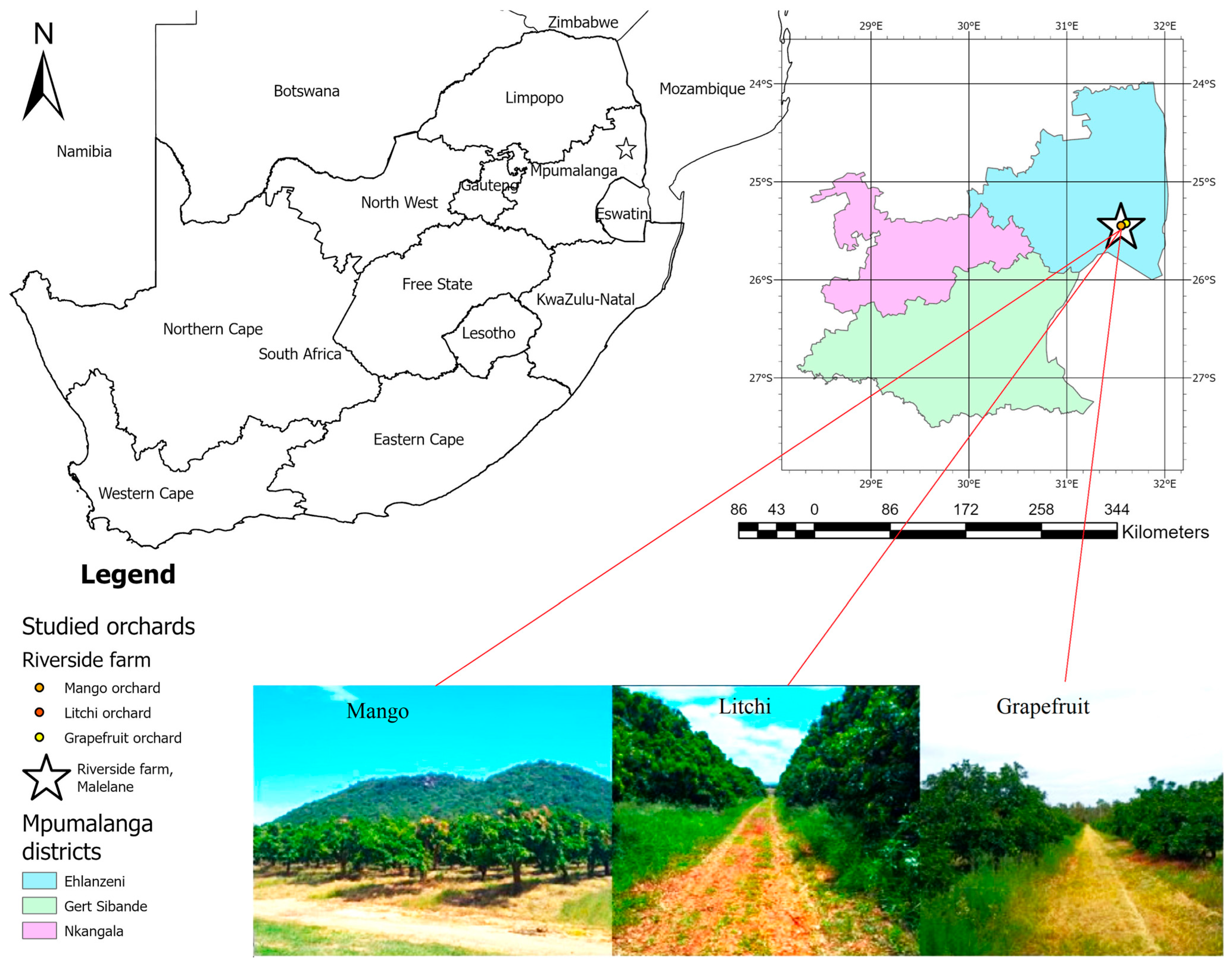
Figure 1. Study site in Malelane, Mpumalanga, South Africa.
Hydrology 12 00189 g001
Figure 2. Development framework for the orchard evapotranspiration partitioning.
Hydrology 12 00189 g002
Figure 3. Normalized difference vegetation index spatial map using Sentinel 2 data for (a) grapefruit, (b) litchi, (c) mango orchards.
Hydrology 12 00189 g003aHydrology 12 00189 g003b
Figure 4. Performance of the Bayesian optimized LightGBM learning model in predicting transpiration using 10-fold cross-validation for (a) litchi, (b) grapefruit, (c) mango, and the corresponding model independent validation for (d) litchi, (e) grapefruit, (f) mango, respectively.
Hydrology 12 00189 g004aHydrology 12 00189 g004b
Figure 5. Performance of the Bayesian optimized LightGBM learning model in predicting evapotranspiration using 10-fold cross-validation for (a) litchi, (b) grapefruit, (c) mango, and the corresponding model independent validation for (d) litchi, (e) grapefruit, (f) mango, respectively.
Hydrology 12 00189 g005aHydrology 12 00189 g005b
Figure 6. SHAP summary plot of the transpiration prediction for (a) litchi, (b) grapefruit, (c) mango.
Hydrology 12 00189 g006aHydrology 12 00189 g006b
Figure 7. SHAP summary plot of the evapotranspiration prediction for (a) litchi, (b) grapefruit, (c) mango.
Hydrology 12 00189 g007aHydrology 12 00189 g007b
Figure 8. The derived orchard partitioning information showing, (a) litchi E T components and E T o , (b) grapefruit E T components and E T o , (c) mango E T components and E T o , (d) litchi crop coefficients, (e) grapefruit crop coefficients, (f) mango crop coefficients, (g) litchi evapotranspiration partition, (h) grapefruit evapotranspiration partition, and (i) mango evapotranspiration partition.
Hydrology 12 00189 g008
Table 1. Crop type, cultivar, rootstock, plant material information, and irrigation method used.
Crop TypeCultivarRootstockAge (yrs)Orchard Size (ha)Number of Plants per HectareTree Height (m)Irrigation System
GrapefruitStar RubyC35/5×5B146.254762.90Microsprinkler
LitchiMauritiusMauritius5313.10706.30Microsprinkler
MangoTommy Atkins-399.503034.70Microsprinkler
Table 2. Normalized difference vegetation index ( N D V I ) maximum, mean, minimum and standard deviation values for grapefruit, litchi and mango orchards.
GrapefruitLitchiMango
Minimum N D V I 0.320.190.30
Maximum N D V I 0.640.820.80
Mean N D V I 0.530.590.63
N D V I Standard deviation0.040.110.06
Table 3. Orchard evapotranspiration measurement campaigns.
OrchardEvapotranspiration Measurement Campaign Period
Grapefruit6–9 December 2022; 7–21 March 2023
Litchi16–31 July 2022; 20 September 2022–18 October 2022; 14 November 2022–1 December 2022
Mango3–28 March 2022; 11 April 2022–30 May 2022; 26 June 2022–3 July 2022
Table 4. Daily maximum and minimum temperature (Tx and Tn), orchard leaf indices (grapefruit, litchi, and mango LAI), total rainfall and reference evapotranspiration (Rain and ETo), average relative humidity, solar radiation, and windspeed at 2 m height (RH, Rs, and Uavg) at the Riverside farm site.
Date
(m/yy)
Rs
(MJ/m2/d)
Tx
(°C)
Tn
(°C)
RH
(%)
Rain
(mm)
Uavg
(m/s)
ETo
(mm)
Grapefruit LAI
(m2/m2)
Litchi LAI
(m2/m2)
Mango LAI
(m2/m2)
Oct-2115.541.09.765.528.71.1120.71.52.13.1
Nov-2117.539.113.073.1137.71.2125.03.25.33.1
Dec-2117.539.116.378.1138.41.0128.73.04.73.1
Jan-2218.835.118.379.7203.21.1133.22.84.23.2
Feb-2221.039.418.472.34.81.2138.02.63.83.2
Mar-2216.838.316.373.484.61.1120.82.13.54.3
Apr-2213.937.412.174.169.31.292.23.14.74.7
May-2212.333.010.876.0113.01.177.03.14.34.3
Jun-2212.228.27.068.45.81.471.14.34.84.4
Jul-2212.930.47.970.04.31.277.52.23.93.7
Aug-2215.134.47.762.93.81.3100.01.62.62.3
Sep-2216.638.69.360.631.01.3121.11.62.22.9
Oct-2216.543.016.267.80.81.4134.92.02.43.1
Nov-2217.437.614.773.837.11.3125.92.42.63.3
Dec-2218.239.815.474.081.31.3139.63.02.73.5
Jan-2320.539.816.171.762.21.3155.33.73.23.0
Feb-2315.934.515.679.4461.41.2108.03.03.43.1
Mar-2318.736.915.275.88.91.1129.22.53.83.3
Apr-2315.638.414.871.330.21.0102.41.63.12.6
May-2311.634.111.777.163.21.074.02.84.42.3
Jun-2312.729.410.864.02.01.272.32.53.22.0
Jul-2312.031.58.563.947.81.377.71.63.32.1
Aug-2318.032.37.963.101.4107.01.73.02.2
Sept-2319.139.110.059.647.91.5133.01.52.22.1
Table 5. Optimal parameters of the transpiration and evapotranspiration LightGBM models.
Parameter NameLitchi TLitchi ETGrapefruit TGrapefruit ETMango TMango ET
n_estimators851997718871483583
max_depth271746244426
learning_rate0.01010.10500.23690.10150.072700.07622
num_leaves922251831824099
lambda_l11.671 × 10−40.098430.47121.415 × 10−60.11320.2037
lambda_l21.8145.002 × 10−80.16771.171 × 10−31.969 × 10−52.231 × 10−5
bagging_fraction0.88480.42720.98500.66670.97010.6694
bagging_freq225265
feature_fraction0.92340.59670.96250.73560.97940.7260
max_bin4721564170173108
min_child_samples8786762850100
min_samples_leaf315269
Disclaimer/Publisher’s Note: The statements, opinions and data contained in all publications are solely those of the individual author(s) and contributor(s) and not of MDPI and/or the editor(s). MDPI and/or the editor(s) disclaim responsibility for any injury to people or property resulting from any ideas, methods, instructions or products referred to in the content.