


Mapping of Closed Depressions in Karst Terrains: A GIS-Based Delineation of Endorheic Catchments in the Alburni Massif (Southern Apennine, Italy)


Abstract
1. Introduction
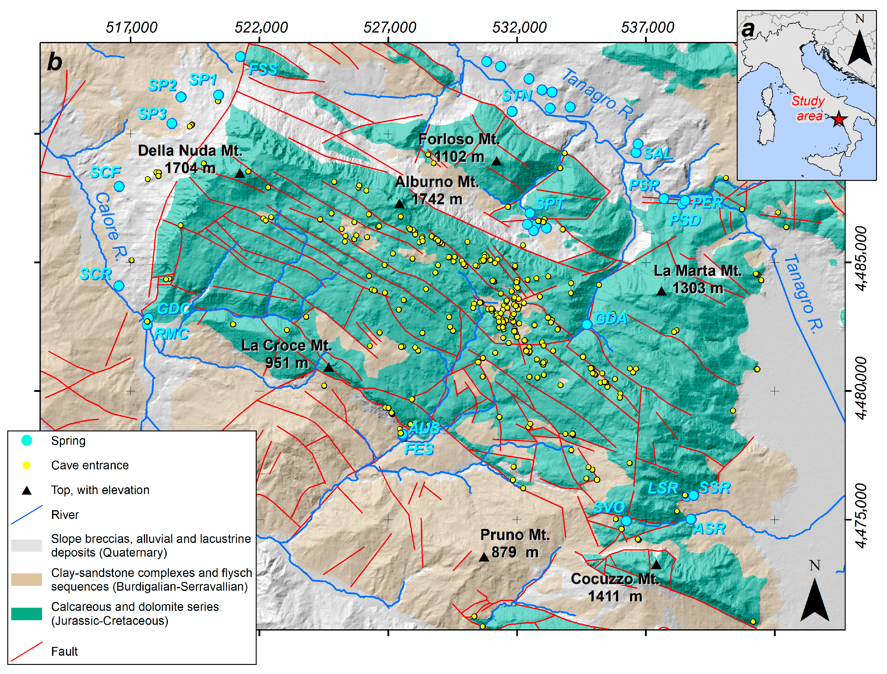
2. Study Area
3. Materials and Methods
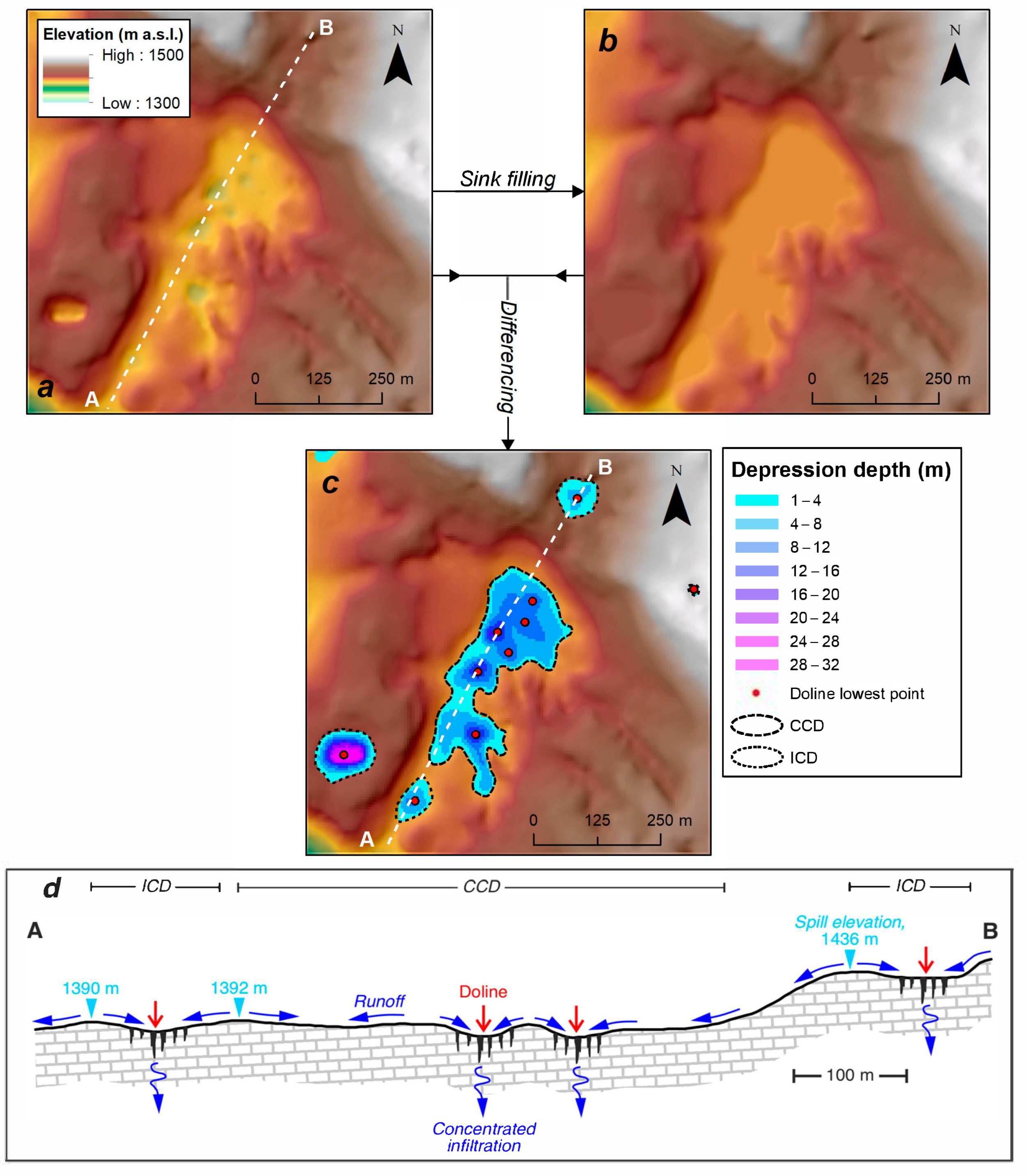
3.1. Types of Karst Closed Depressions
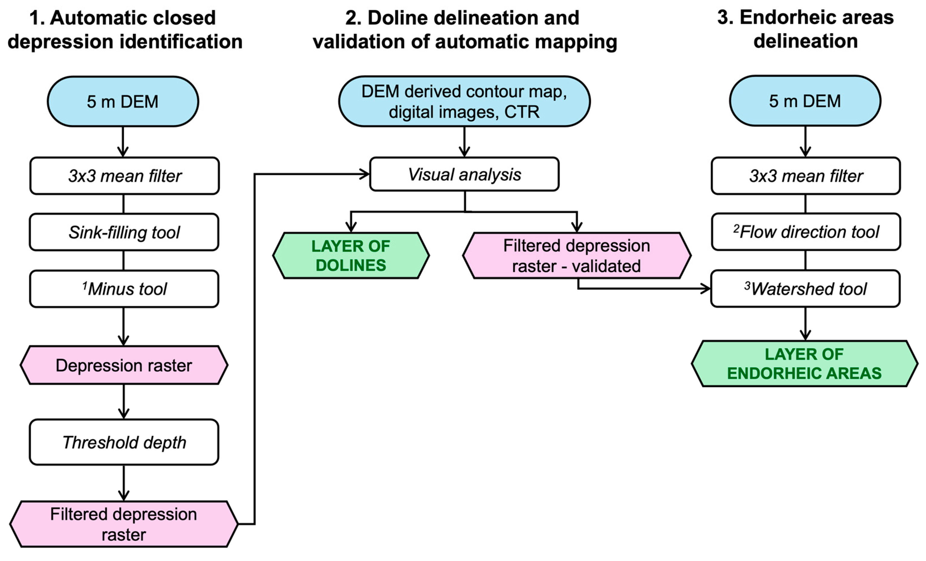
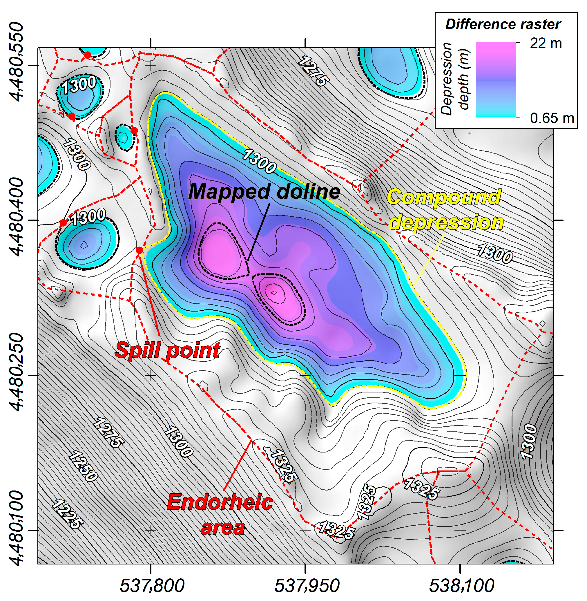
3.2. Closed Depression Mapping
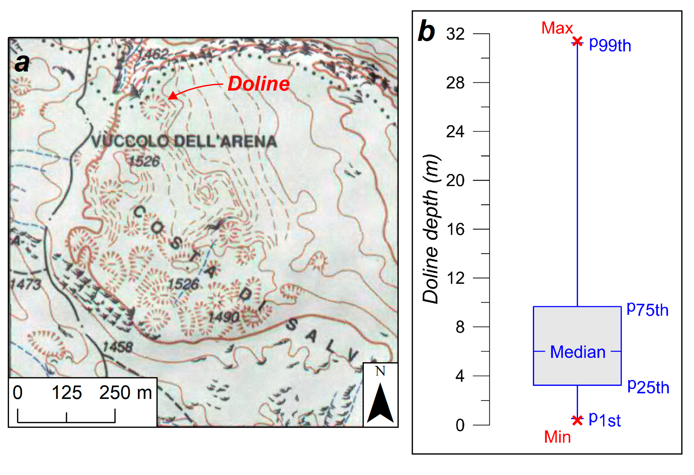
3.3. Doline Mapping
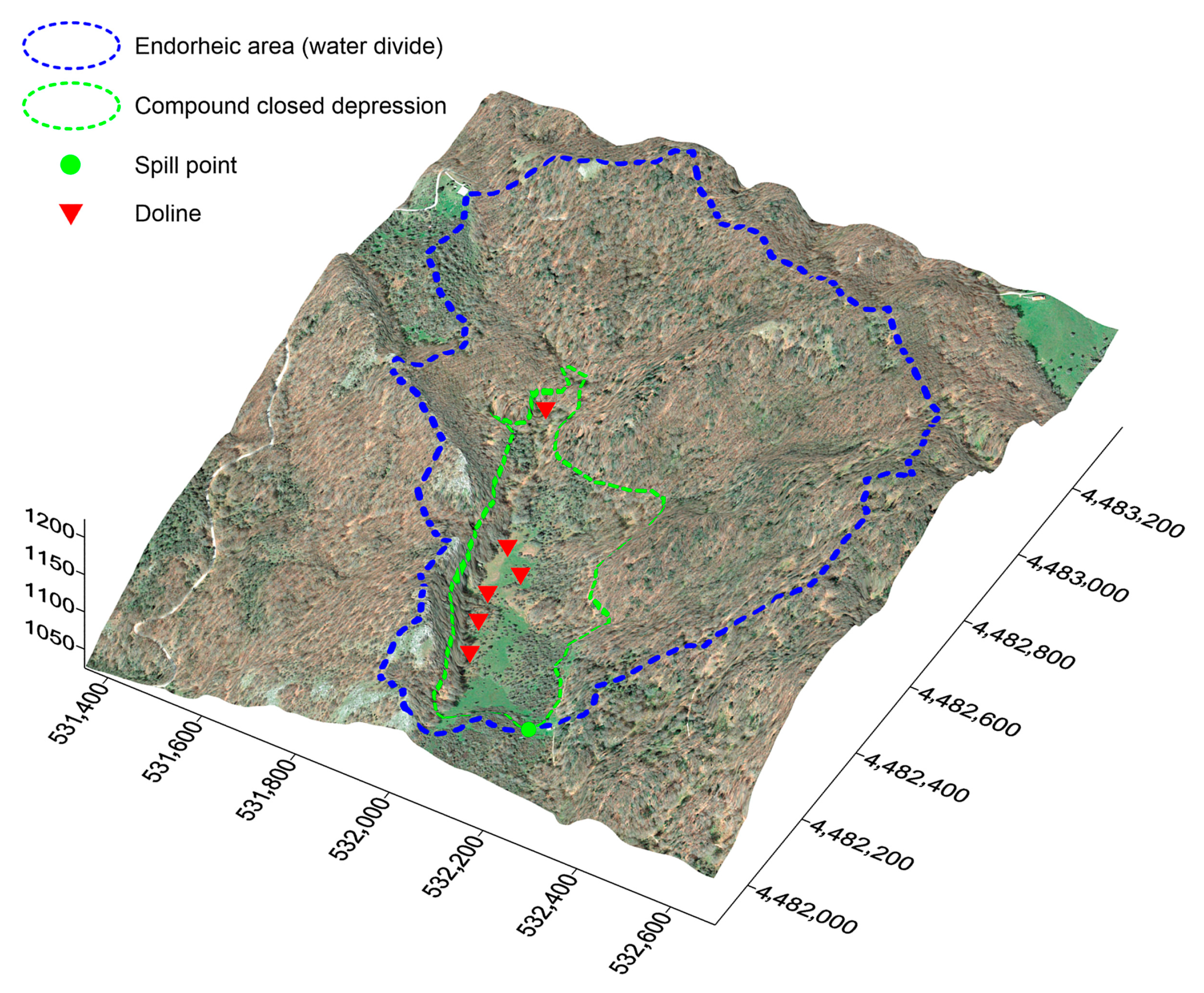
3.4. Automatic Mapping of Endorheic Areas
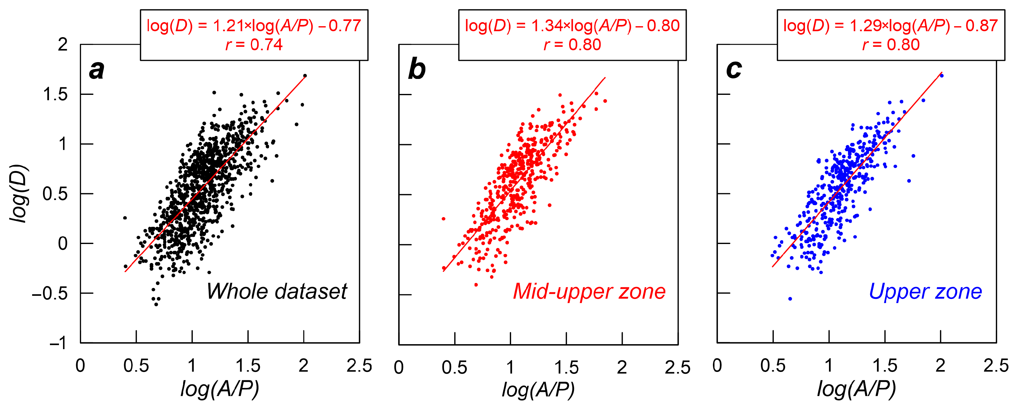
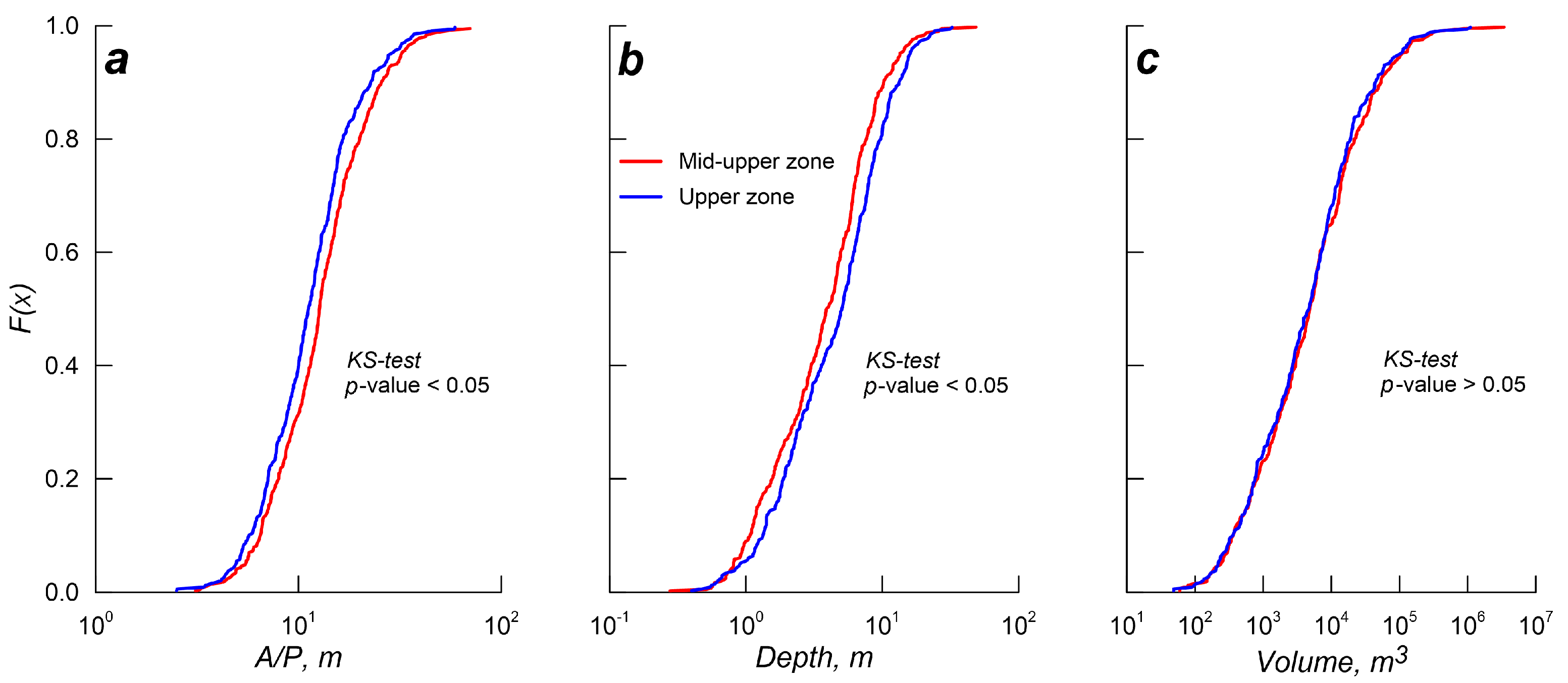
3.5. Morphometric Parameters
4. Results
5. Discussion
6. Conclusions
Author Contributions
Funding
Data Availability Statement
Acknowledgments
Conflicts of Interest
References
- Šegina, E.; Benac, Č.; Rubinić, J.; Knez, M. Morphometric Analyses of Dolines—The Problem of Delineation and Calculation of Basic Parameters. Acta Carsologica 2018, 47, 23–33. [Google Scholar] [CrossRef]
- Bondesan, A.; Meneghel, M.; Sauro, U. Morphometri Analysis of Dolines. Int. J. Speleol. 1992, 21, 1–55. [Google Scholar] [CrossRef]
- Wu, Q.; Deng, C.; Chen, Z. Automated Delineation of Karst Sinkholes from LiDAR-Derived Digital Elevation Models. Geomorphology 2016, 266, 1–10. [Google Scholar] [CrossRef]
- Kozar, M.D.; McCoy, K.J.; Weary, D.J.; Field, M.S.; Pierce, H.A.; Schill, W.B.; Joung, J.A. Geohydrology and Water Quality of the Leetown Area, West Virginia; U.S. Geological Survey Open-file Report; U.S. Geological Survey: Raystown, WV, USA, 2007.
- Doctor, D.H.; Young, J.A. An Evaluation of Automated GIS Tools for Delineating Karst Sinkholes and Closed Depressions From 1-Meter Lidar-Derived Digital Elevation Data. In Proceedings of the 13th Multidisciplinary Conference on Sinkholes and the Engineering and Environmental Impacts of Karst, Carlsbad, NM, USA, 6–10 May 2013; pp. 449–458. [Google Scholar]
- Hofierka, J.; Gallay, M.; Bandura, P.; Šašak, J. Identification of Karst Sinkholes in a Forested Karst Landscape Using Airborne Laser Scanning Data and Water Flow Analysis. Geomorphology 2018, 308, 265–277. [Google Scholar] [CrossRef]
- Čeru, T.; Šegina, E.; Gosar, A. Geomorphological Dating of Pleistocene Conglomerates in Central Slovenia Based on Spatial Analyses of Dolines Using LiDAR and Ground Penetrating Radar. Remote Sens. 2017, 9, 1213. [Google Scholar] [CrossRef]
- Stefanovski, S.; Kokalj, Ž.; Stepišnik, U. Sky-View Factor Enhanced Doline Delineation: A Comparative Methodological Review Based on Case Studies in Slovenia. Geomorphology 2024, 465, 109389. [Google Scholar] [CrossRef]
- Moreno-Gómez, M.; Liedl, R.; Stefan, C. A New GIS-Based Model for Karst Dolines Mapping Using LiDAR; Application of a Multidepth Threshold Approach in the Yucatan Karst, Mexico. Remote Sens. 2019, 11, 1147. [Google Scholar] [CrossRef]
- Andreo, B.; Vías, J.; Durán, J.J.; Jiménez, P.; López-Geta, J.A.; Carrasco, F. Methodology for Groundwater Recharge Assessment in Carbonate Aquifers: Application to Pilot Sites in Southern Spain. Hydrogeol. J. 2008, 16, 911–925. [Google Scholar] [CrossRef]
- Goldscheider, N.; Meiman, J.; Pronk, M.; Smart, C. Tracer Tests in Karst Hydrogeology and Speleology. Int. J. Speleol. 2008, 37, 27–40. [Google Scholar] [CrossRef]
- Goldscheider, N. Delineation of Spring Protection Zones. In Groundwater Hydrology of Springs; Krasic, N., Stevanovic, Z., Eds.; 2010; pp. 305–338. [Google Scholar]
- Gutiérrez, F.; Galve, J.P.; Lucha, P.; Castañeda, C.; Bonachea, J.; Guerrero, J. Integrating Geomorphological Mapping, Trenching, InSAR and GPR for the Identification and Characterization of Sinkholes: A Review and Application in the Mantled Evaporite Karst of the Ebro Valley (NE Spain). Geomorphology 2011, 134, 144–156. [Google Scholar] [CrossRef]
- Gutiérrez, F.; Parise, M.; De Waele, J.; Jourde, H. A Review on Natural and Human-Induced Geohazards and Impacts in Karst. Earth-Sci. Rev. 2014, 138, 61–88. [Google Scholar] [CrossRef]
- Fiorillo, F.; Pagnozzi, M.; Ventafridda, G. A Model to Simulate Recharge Processes of Karst Massifs. Hydrol. Process. 2015, 29, 2301–2314. [Google Scholar] [CrossRef]
- Fiorillo, F.; Pagnozzi, M.; Addesso, R.; Cafaro, S.; D’Angeli, I.M.; Esposito, L.; Leone, G.; Liso, I.S.; Parise, M. Uncertainties in Understanding Groundwater Flow and Spring Functioning in Karst. In Geophysical Monograph Series; Currell, M.J., Katz, B.G., Eds.; Wiley: New York, NY, USA, 2022; pp. 131–143. ISBN 978-1-119-81859-5. [Google Scholar]
- Marín, A.I.; Martín Rodríguez, J.F.; Barberá, J.A.; Fernández-Ortega, J.; Mudarra, M.; Sánchez, D.; Andreo, B. Groundwater Vulnerability to Pollution in Karst Aquifers, Considering Key Challenges and Considerations: Application to the Ubrique Springs in Southern Spain. Hydrogeol. J. 2021, 29, 379–396. [Google Scholar] [CrossRef]
- Palmer, A.N. Origin and Morphology of Limestone Caves. Geol. Soc. Am. Bull. 1991, 103, 1–21. [Google Scholar] [CrossRef]
- Klimchouk, A.B. Hypogene Speleogenesis: Hydrogeological and Morphogenetic Perspective; Special paper/National Cave and Karst Research Institute; National Cave and Karst Research Inst: Carlsbad, NM, USA, 2007; ISBN 978-0-9795422-0-6. [Google Scholar]
- Leone, G.; Catani, V.; Pagnozzi, M.; Ginolfi, M.; Testa, G.; Esposito, L.; Fiorillo, F. Hydrological Features of Matese Karst Massif, Focused on Endorheic Areas, Dolines and Hydroelectric Exploitation. J. Maps 2022, 19, 2144497. [Google Scholar] [CrossRef]
- Gutiérrez, F.; Guerrero, J.; Lucha, P. A Genetic Classification of Sinkholes Illustrated from Evaporite Paleokarst Exposures in Spain. Environ. Geol. 2008, 53, 993–1006. [Google Scholar] [CrossRef]
- Gunn, J. Point-Recharge of Limestone Aquifers—A Model from New Zealand Karst. J. Hydrol. 1983, 61, 19–29. [Google Scholar] [CrossRef]
- Sauro, U. Closed Depressions in Karst Areas. In Encyclopedia of Caves; Academic Press: Cambridge, MA, USA, 2012; pp. 140–155. [Google Scholar]
- Klingseisen, B.; Metternicht, G.; Paulus, G. Geomorphometric Landscape Analysis Using a Semi-Automated GIS-Approach. Environ. Model. Softw. 2008, 23, 109–121. [Google Scholar] [CrossRef]
- Bonacci, O.; Andrić, I. Karst Spring Catchment: An Example from Dinaric Karst. Environ. Earth Sci. 2015, 74, 6211–6223. [Google Scholar] [CrossRef]
- White, W.B. Karst Hydrology: Recent Developments and Open Questions. Eng. Geol. 2002, 65, 85–105. [Google Scholar] [CrossRef]
- Valente, A.; Catani, V.; Esposito, L.; Leone, G.; Pagnozzi, M.; Fiorillo, F. Groundwater Resources in a Complex Karst Environment Involved by Wind Power Farm Construction. Sustainability 2022, 14, 11975. [Google Scholar] [CrossRef]
- Santo, A.; Giulivo, I.; Russo, N.; Prete, S. Grotte e Speleologia Della Campania; Elio Sellino editore: Avellino, Italy, 2005; ISBN 88-88991-32-8. [Google Scholar]
- Brancaccio, L.; Civita, M.; Vallario, A. Prime Osservazioni Sui Problemi Idrogeologici Dell’Alburno (Campania). Boll. Della Soc. Geol. Dei Nat. Napoli 1973, 82, 13–35. [Google Scholar]
- Scandone, P. Studi Di Geologia Lucana: Carta Dei Terreni Della Serie Calcareo-Silico-Marnosa e Note Illustrative. Boll. Soc. Nat. 1972, 81, 225–300. [Google Scholar]
- Ippolito, F.; Ortolani, F.; Russo, M. Struttura Marginale Tirrenica Dell’Appennino Campano: Reinterpretazione Di Dati Di Antiche Ricerche Di Idrocarburi. Mem. Della Soc. Geol. Ital. 1973, 12, 227–250. [Google Scholar]
- Patacca, E.; Scandone, P. Geology of the Southern Apennines. Ital. J. Geosci. 2007, 7, 75–112. [Google Scholar]
- Pagnozzi, M.; Fiorillo, F.; Esposito, L.; Leone, G. Hydrological Features of Endorheic Areas in Southern Italy. Ital. J. Eng. Geol. Environ. 2019, 85–91. [Google Scholar] [CrossRef]
- Fiorillo, F. Spring Hydrographs as Indicators of Droughts in a Karst Environment. J. Hydrol. 2009, 373, 290–301. [Google Scholar] [CrossRef]
- Bellucci, F.; Giulivo, I.; Pelella, L.; Santo, A. Carsismo Ed Idrogeologia Del Settore Centrale Dei Mt. Alburni (Sa). Geol. Tec. 1991, 3, 5–12. [Google Scholar]
- Bellucci, F.; Giulivo, I.; Pelella, L.; Santo, A. Monti Alburni: Ricerche Speleologiche; De Angelis: Rome, Italy, 1995. [Google Scholar]
- Celico, P.; Pelella, L.; Stanzione, D.; Aquino, S. Sull’idrogeologia e l’idrogeochimica Dei Monti Alburni. Geol. Romana 1994, 30, 687–698. [Google Scholar]
- Ducci, D.; De Masi, G.; Delli Priscoli, G. Contamination Risk of the Alburni Karst System (Southern Italy). Eng. Geol. 2008, 99, 109–120. [Google Scholar] [CrossRef]
- Santo, A. Idrogeologia Dell’area Carsica Di Castelcivita (M. Alburni-SA). Geol. Appl. Idrogeol. 1993, 27, 663–673. [Google Scholar]
- Bolognini, M.; Celico, P.; Tescione, M.; Aquino, S. La Produttività Deii Pozzi in Acquiferi Carbonatici Molto Carsificati: L’esempio Dei Monti Alburni (SA). Geol. Romana 1994, 30, 671–686. [Google Scholar]
- Bonacci, O. Karst Hydrology with Special References to the Dinaric Karst; Springer: Berlin/Heidelberg, Germany, 1987. [Google Scholar]
- Klimchouk, A. The Formation of Epikarst and Its Role in Vadose Speleogenesis. In Speleogenesis: Evolution of Karst Aquifers; National Speleological Society: Huntsville, AL, USA, 2000. [Google Scholar]
- Veress, M. Covered Karsts; Springer Geology: Dordrecht, The Netherlands, 2016; ISBN 978-94-017-7516-8. [Google Scholar]
- Ford, D.; Williams, P. Karst Hydrogeology and Geomorphology; John Wiley & Sons Ltd.: West Sussex, UK, 2007; ISBN 978-1-118-68498-6. [Google Scholar]
- Ćalić, J. Karstic Uvala Revisited: Toward a Redefinition of the Term. Geomorphology 2011, 134, 32–42. [Google Scholar] [CrossRef]
- Gams, I. The polje; The problem of definition; With special regard to the Dinaric karst. Z. Fuer Geomorphol. 1978, 22, 170–181. [Google Scholar]
- Bonacci, O. 6.11 Poljes, Ponors and Their Catchments. In Treatise on Geomorphology; Elsevier: Amsterdam, The Netherlands, 2013; pp. 112–120. ISBN 978-0-08-088522-3. [Google Scholar]
- Field, M. Lexicon of Cave and Karst Terminology with Special Reference to Environmental Karst Hydrology; EPA National Center for Environmental Assessment: Washington, DC, USA, 2002; p. 214.
- De Carvalho, O.; Guimarães, R.; Montgomery, D.; Gillespie, A.; Trancoso Gomes, R.; De Souza Martins, É.; Silva, N. Karst Depression Detection Using ASTER, ALOS/PRISM and SRTM-Derived Digital Elevation Models in the Bambuí Group, Brazil. Remote Sens. 2013, 6, 330–351. [Google Scholar] [CrossRef]
- O’Callaghan, J.F.; Mark, D.M. The Extraction of Drainage Networks from Digital Elevation Data. Comput. Vis. Graph. Image Process. 1984, 28, 323–344. [Google Scholar] [CrossRef]
- Planchon, O.; Darboux, F. A Fast, Simple and Versatile Algorithm to Fill the Depressions of Digital Elevation Models. Catena 2002, 46, 159–176. [Google Scholar] [CrossRef]
- Wang, L.; Liu, H. An Efficient Method for Identifying and Filling Surface Depressions in Digital Elevation Models for Hydrologic Analysis and Modelling. Int. J. Geogr. Inf. Sci. 2006, 20, 193–213. [Google Scholar] [CrossRef]
- Verbovšek, T.; Gabor, L. Morphometric Properties of Dolines in Matarsko Podolje, SW Slovenia. Environ. Earth Sci. 2019, 78, 396. [Google Scholar] [CrossRef]
- Bauer, C. Analysis of Dolines Using Multiple Methods Applied to Airborne Laser Scanning Data. Geomorphology 2015, 250, 78–88. [Google Scholar] [CrossRef]
- Fiorillo, F.; Pagnozzi, M. Recharge Processes of Matese Karst Massif (Southern Italy). Environ. Earth Sci. 2015, 74, 7557–7570. [Google Scholar] [CrossRef]
- Troester, J.W.; White, E.L.; White, W.B. A comparison of sinkhole depth frequency distributions in temperate and tropical karst regions. In Sinkholes: Their geology, engineering, and environmental impact; Beck, B.F., Ed.; Balkema: Rotterdam, The Netherlands, 1984; pp. 65–73. [Google Scholar]
- Fiorillo, F.; Leone, G.; Pagnozzi, M.; Catani, V.; Testa, G.; Esposito, L. The Upwelling Groundwater Flow in the Karst Area of Grassano-Telese Springs (Southern Italy). Water 2019, 11, 872. [Google Scholar] [CrossRef]
- Caramanna, G.; Ciotoli, G.; Nisio, S. A Review of Natural Sinkhole Phenomena in Italian Plain Areas. Nat. Hazards 2008, 45, 145–172. [Google Scholar] [CrossRef]
- Borradaile, G. Statistics of Earth Science Data: Their Distribution in Time, Space, and Orientation; Springer: Berlin/Heidelberg, Germany, 2003; ISBN 978-3-642-07815-6. [Google Scholar]
- Santangelo, N.; Santo, A. Endokarst Processes in the Alburni Massif (Campania, Southern Italy): Evolution of Ponors and Hydrogeological Implications. Z. Für Geomorphol. 1997, 41, 229–247. [Google Scholar] [CrossRef]
- Santo, A. Alcune Osservazioni Sul Carsismo Ipogeo Dei M. Alburni. Appennino Meridionale Annu. Club Alpino Ital. Sez. Napoli 1988, 1, 71–88. [Google Scholar]
- Incoronato, A.; Nardi, G.; Ortolani, F. Assetto Strutturale Dei Massicci Carbonatici Della Campania Meridionale. Implicazioni Idrogeologiche. Rend. Accad. Sci. Fis. E Mat. Della Soc. Naz. Sci. Lett. E Arti Napoli 1978, 45, 479–493. [Google Scholar]
- Aucelli, P.P.C.; Cesarano, M.; Di Paola, G.; Filocamo, F.; Rosskopf, C.M. Geomorphological Map of the Central Sector of the Matese Mountains (Southern Italy): An Example of Complex Landscape Evolution in a Mediterranean Mountain Environment. J. Maps 2013, 9, 604–616. [Google Scholar] [CrossRef]
- Zumpano, V.; Pisano, L.; Parise, M. An Integrated Framework to Identify and Analyze Karst Sinkholes. Geomorphology 2019, 332, 213–225. [Google Scholar] [CrossRef]
- Jenson, S.K.; Domingue, J.O. Extracting Topographic Structure from Digital Elevation Data for Geographic Information-System Analysis. Photogramm. Eng. Remote Sens. 1988, 54, 1593–1600. [Google Scholar]
- Goldscheider, N. Karst Groundwater Vulnerability Mapping: Application of a New Method in the Swabian Alb, Germany. Hydrogeol. J. 2005, 13, 555–564. [Google Scholar] [CrossRef]
- Goldscheider, N.; Klute, M.; Sturm, S.; Hötzl, H. The PI Method—A GIS-Based Approach to Mapping Groundwater Vulnerability with Special Consideration of Karst Aquifers. Z. Angew. Geol. 2000, 46, 157–166. [Google Scholar]
- Doerfliger, N.; Jeannin, P.-Y.; Zwahlen, F. Water Vulnerability Assessment in Karst Environments: A New Method of Defining Protection Areas Using a Multi-Attribute Approach and GIS Tools (EPIK Method). Environ. Geol. 1999, 39, 165–176. [Google Scholar] [CrossRef]
- Vías, J.M.; Andreo, B.; Perles, M.J.; Carrasco, F.; Vadillo, I.; Jiménez, P. Proposed Method for Groundwater Vulnerability Mapping in Carbonate (Karstic) Aquifers: The COP Method: Application in Two Pilot Sites in Southern Spain. Hydrogeol. J. 2006, 14, 912–925. [Google Scholar] [CrossRef]
- Goldscheider, N.; Drew, D. Methods in Karst Hydrogeology; International Contributions to Hydrogeology; Taylor & Francis: London, UK, 2007; ISBN 978-0-415-42873-6. [Google Scholar]


| Label | Spring Name | Spring Group | Elevation m a.s.l. | Mean Discharge m3/s |
|---|---|---|---|---|
| PSP | Pertosa | Pertosa | 195 | 1.1 |
| SPT | Petina | 647 | 0.1 | |
| PSD | Santa Domenica | 243 | nd | |
| PER | Pertosa Caves | 263 | 1.1 | |
| AUS | Auso Resurgence | Auso | 280 | 1 |
| FES | Festola | 280 | nd | |
| RMC | Mulino di Castelcivita Resurgence | Castelcivita | 65 | nd |
| GDC | Castelcivita Caves | 94 | 1 to 4 | |
| STN | Tanagro | Lower Tanagro | 204 | >8.5 |
| SCR | Controne | Other springs | 100 | 0.1 |
| SP1 | Postiglione 1 | 570 | 0.1 | |
| SP2 | Postiglione 2 | 570 | 0.1 | |
| SP3 | Postiglione 3 | 570 | 0.1 | |
| SCF | Cafaro | 180 | nd | |
| FSS | Fontana Scorzo Sicignano | 363 | 0.01 | |
| SAL | Auletta | 235 | nd | |
| LSR | Lavatoio San Rufo | 669 | 0.01 | |
| SSR | San Rufo | 636 | nd | |
| ASR | Abbotituro San Rufo | 672 | 0.01 | |
| SVO | Valetorno | 848 | nd | |
| GDA | Dell’Acqua Caves | 875 | nd |
| Data | Year | Resolution or Scale | Author or Provider |
|---|---|---|---|
| Digital Elevation Model (DEM) | - | 5 m | - |
| Digital orthophoto | 2006, 2012 | 0.5 m | Geoportale Nazione, Ministero dell’Ambiente e della Sicurezza Energetica (MASE) |
| Google Earth satellite images | 2016–2023 | - | |
| Technical Regional Chart (CTR) | 2004 | 1:5000 | Territorial Informative System of Campania Region |
| Topographic Map | 1995 | 1:25,000 | Italian Military Geographic Institute (IGMI) |
Disclaimer/Publisher’s Note: The statements, opinions and data contained in all publications are solely those of the individual author(s) and contributor(s) and not of MDPI and/or the editor(s). MDPI and/or the editor(s) disclaim responsibility for any injury to people or property resulting from any ideas, methods, instructions or products referred to in the content. |
© 2025 by the authors. Licensee MDPI, Basel, Switzerland. This article is an open access article distributed under the terms and conditions of the Creative Commons Attribution (CC BY) license (https://creativecommons.org/licenses/by/4.0/).
Share and Cite
Esposito, L.; Leone, G.; Ginolfi, M.; Chenari, S.A.; Fiorillo, F. Mapping of Closed Depressions in Karst Terrains: A GIS-Based Delineation of Endorheic Catchments in the Alburni Massif (Southern Apennine, Italy). Hydrology 2025, 12, 186. https://doi.org/10.3390/hydrology12070186
Esposito L, Leone G, Ginolfi M, Chenari SA, Fiorillo F. Mapping of Closed Depressions in Karst Terrains: A GIS-Based Delineation of Endorheic Catchments in the Alburni Massif (Southern Apennine, Italy). Hydrology. 2025; 12(7):186. https://doi.org/10.3390/hydrology12070186
Chicago/Turabian StyleEsposito, Libera, Guido Leone, Michele Ginolfi, Saman Abbasi Chenari, and Francesco Fiorillo. 2025. "Mapping of Closed Depressions in Karst Terrains: A GIS-Based Delineation of Endorheic Catchments in the Alburni Massif (Southern Apennine, Italy)" Hydrology 12, no. 7: 186. https://doi.org/10.3390/hydrology12070186
APA StyleEsposito, L., Leone, G., Ginolfi, M., Chenari, S. A., & Fiorillo, F. (2025). Mapping of Closed Depressions in Karst Terrains: A GIS-Based Delineation of Endorheic Catchments in the Alburni Massif (Southern Apennine, Italy). Hydrology, 12(7), 186. https://doi.org/10.3390/hydrology12070186