
Time-Series Analysis of Monitoring Data from Springs to Assess the Hydrodynamic Characteristics of a Coastal Discharge Zone: Example of Jurjevska Žrnovnica Springs in Croatia


Abstract
1. Introduction
2. Methods
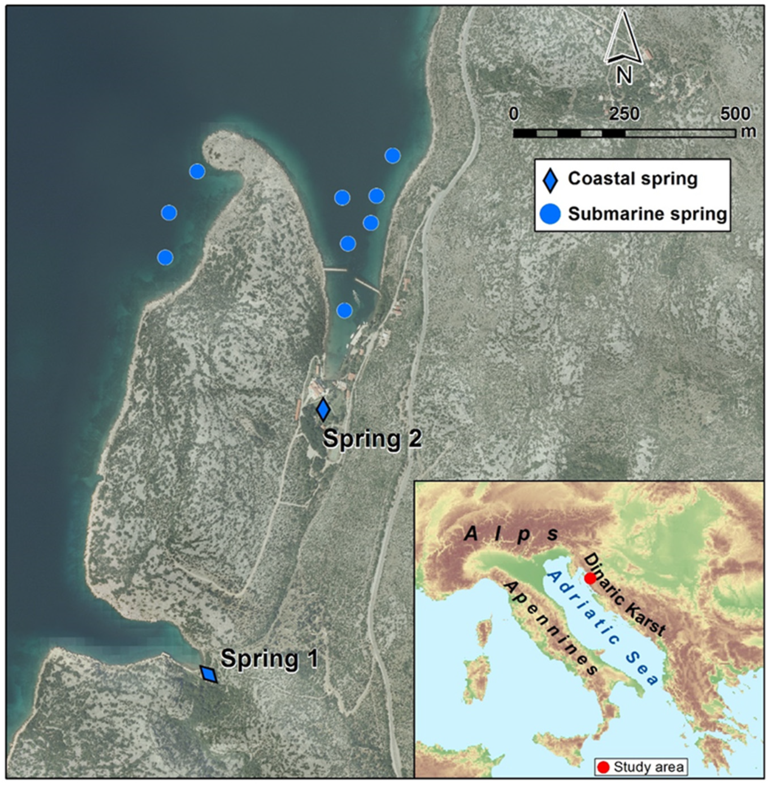
2.1. Data Collection
2.2. Analyses of Complete Hourly Time Series
2.3. Analysis of Daily Data
3. Results
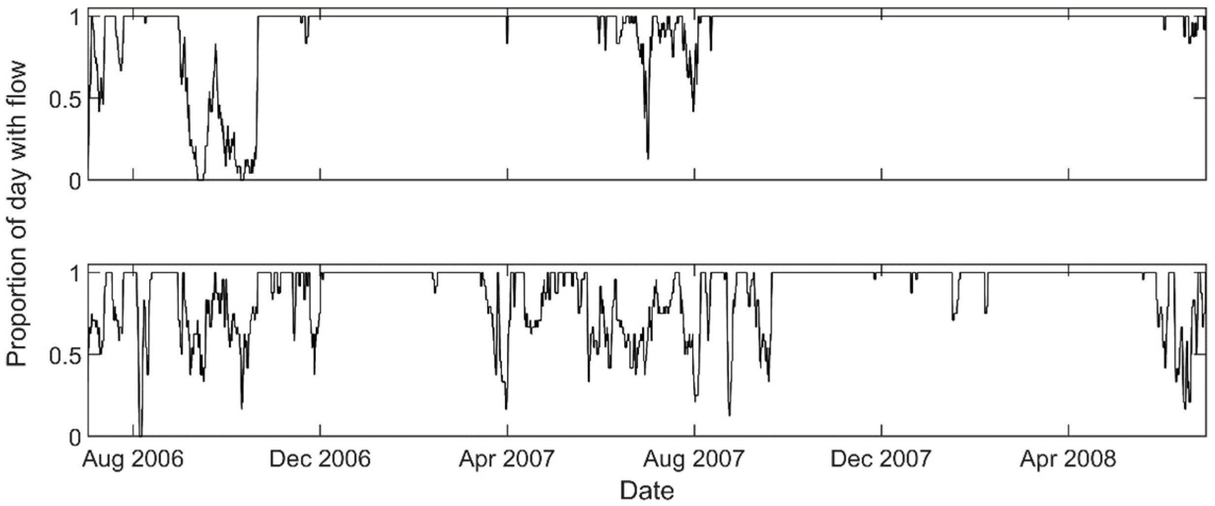
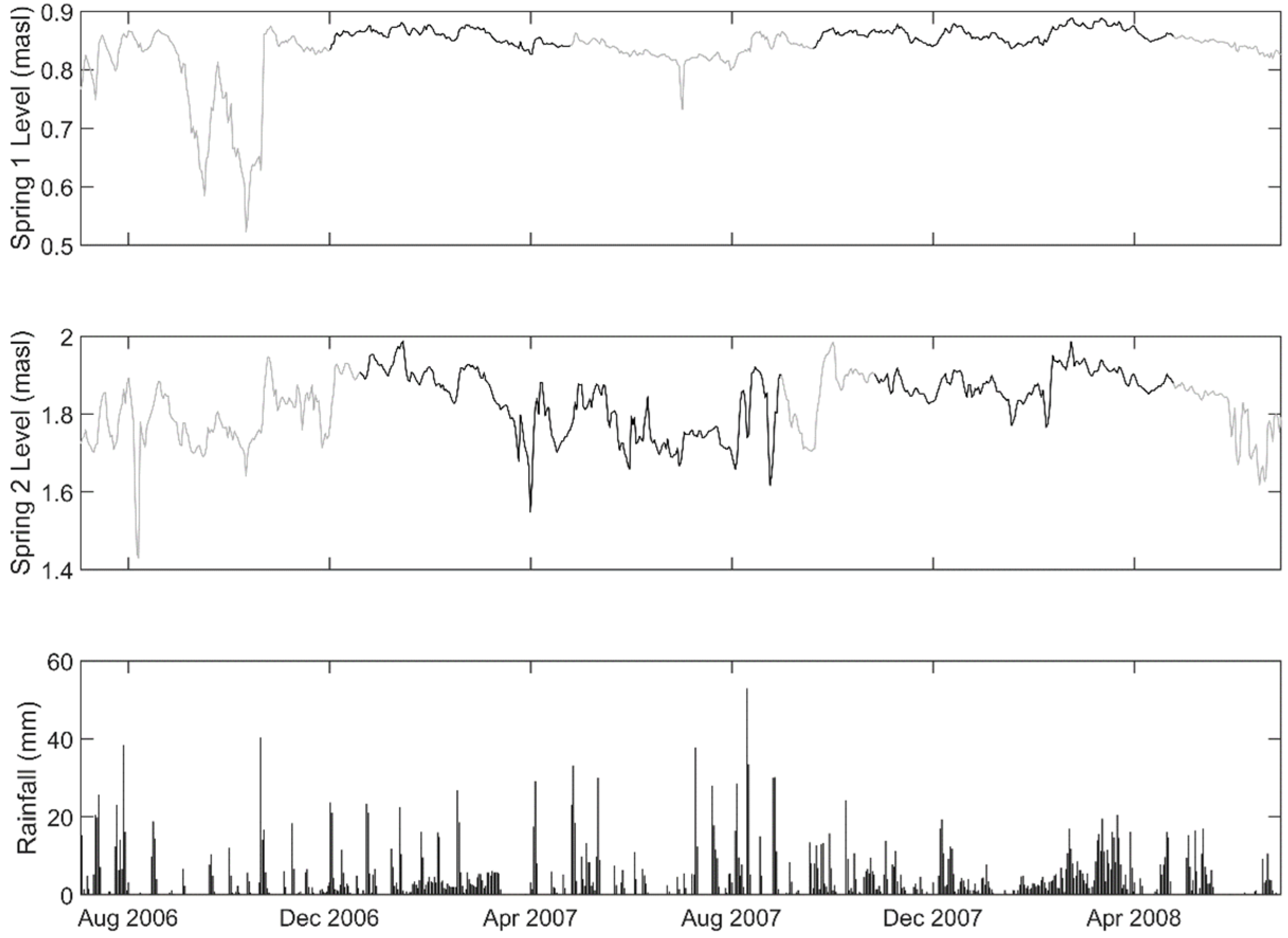
3.1. Data Summary
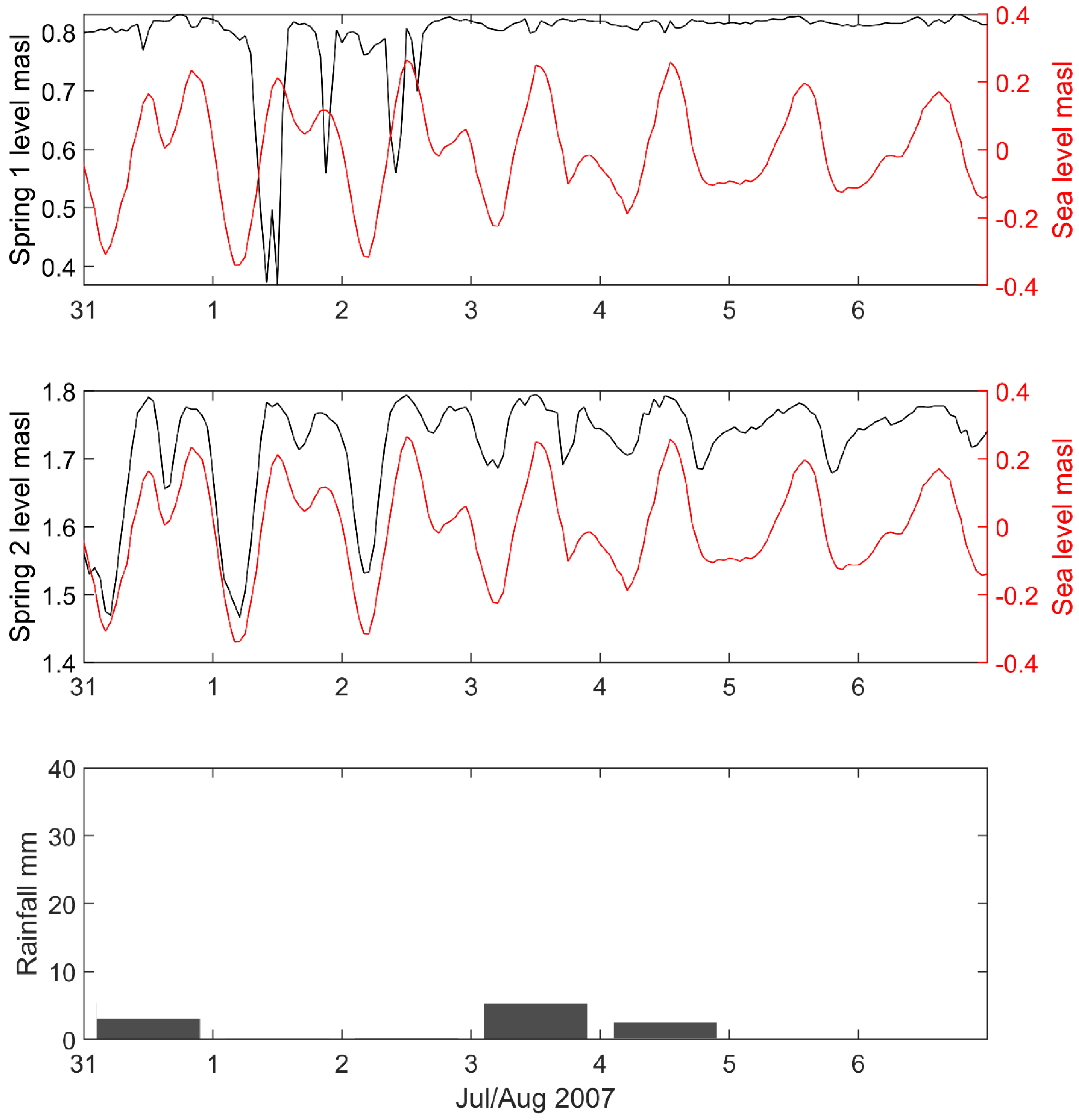
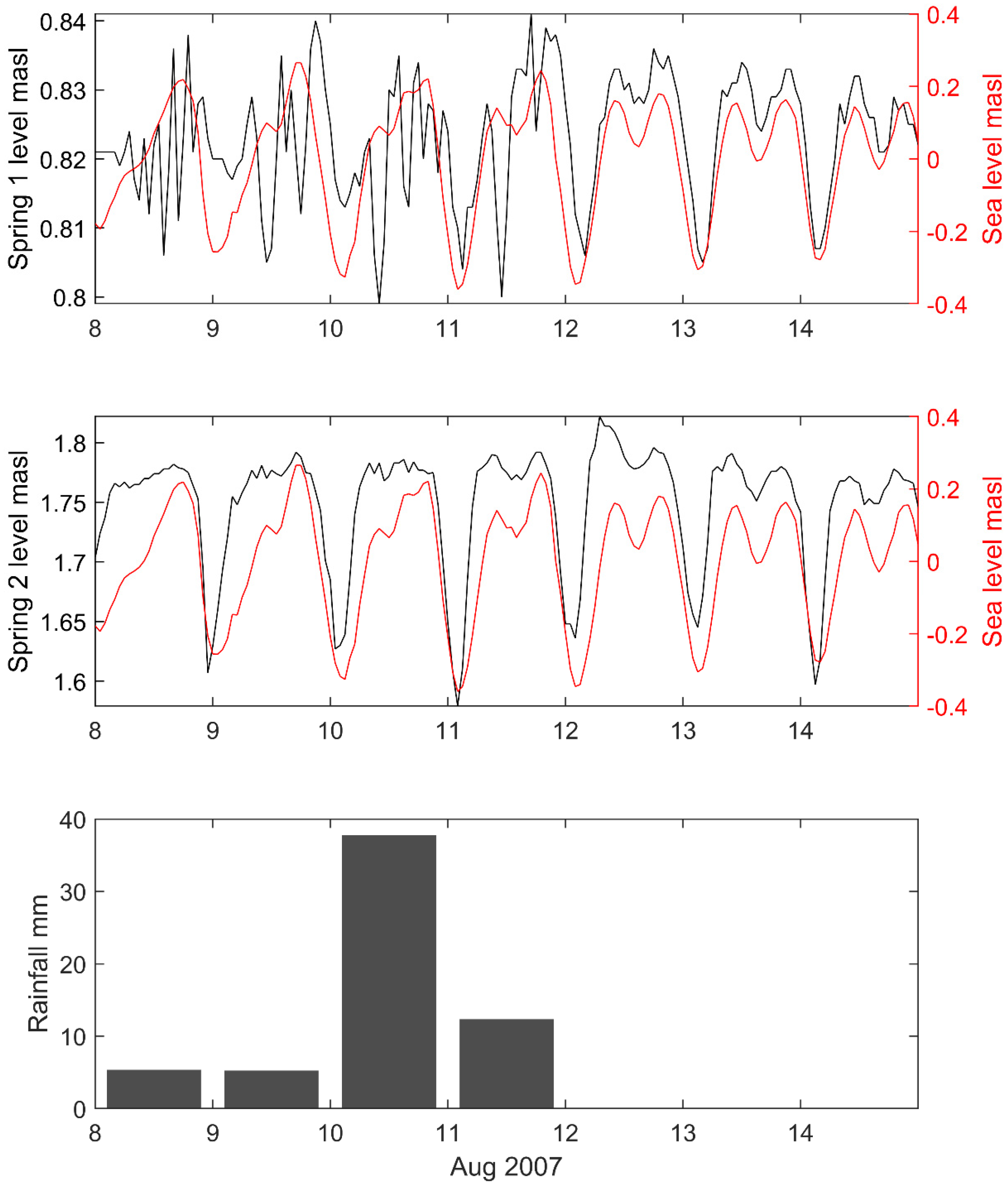
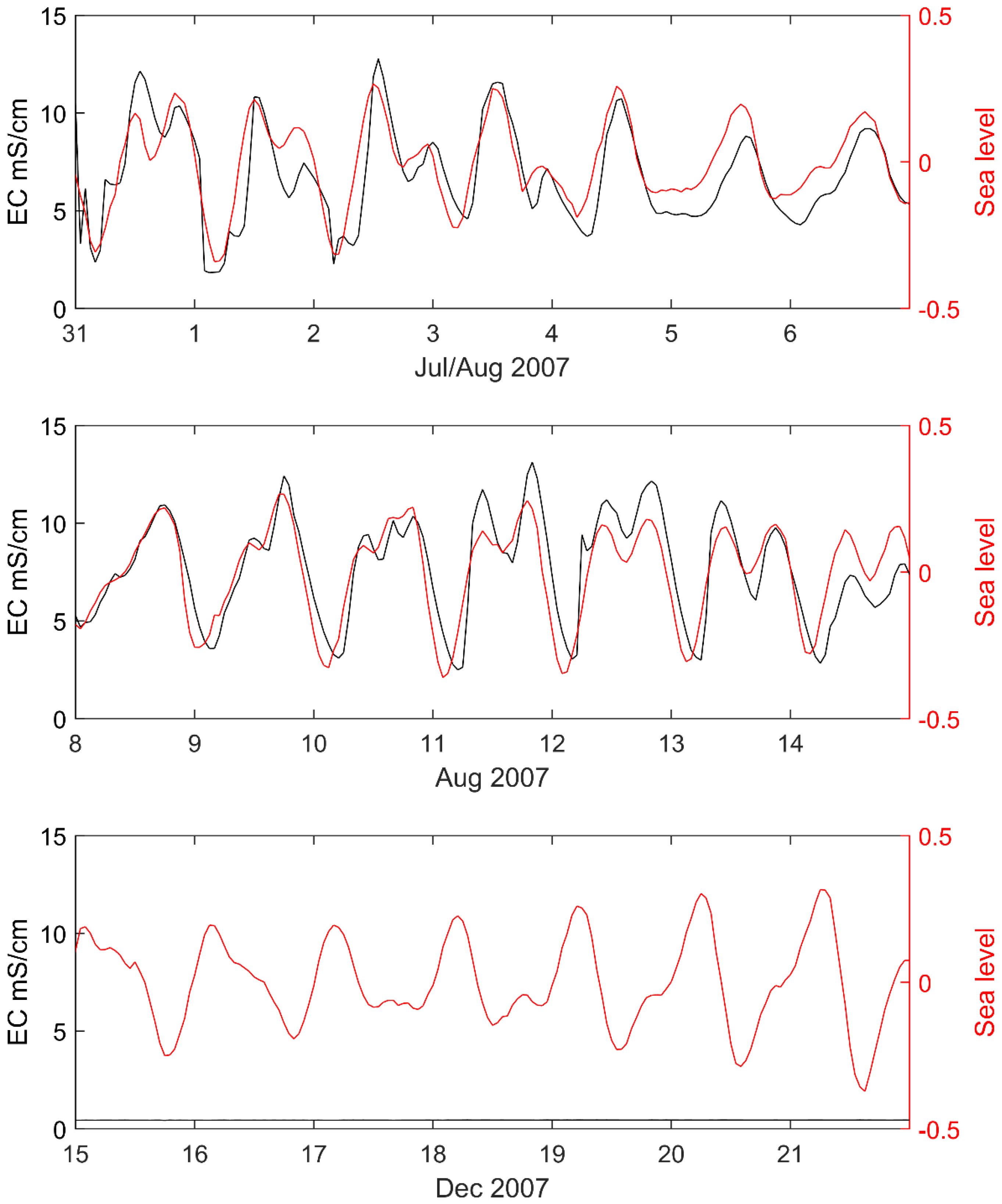
3.2. Analysis of Within-Day Spring and Sea Level Variation
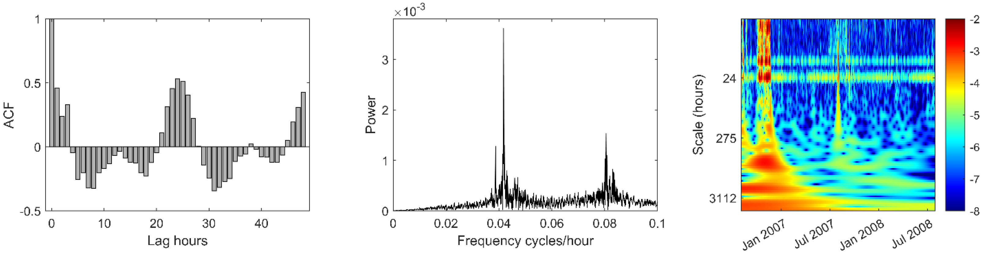
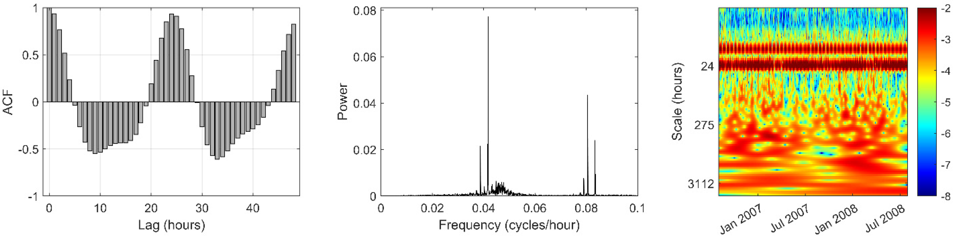
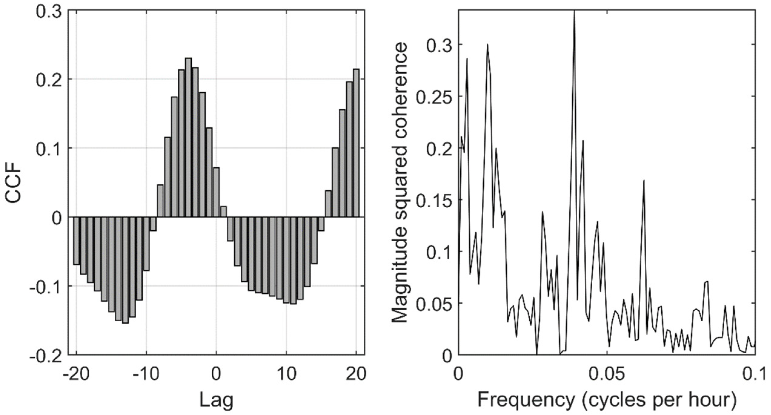
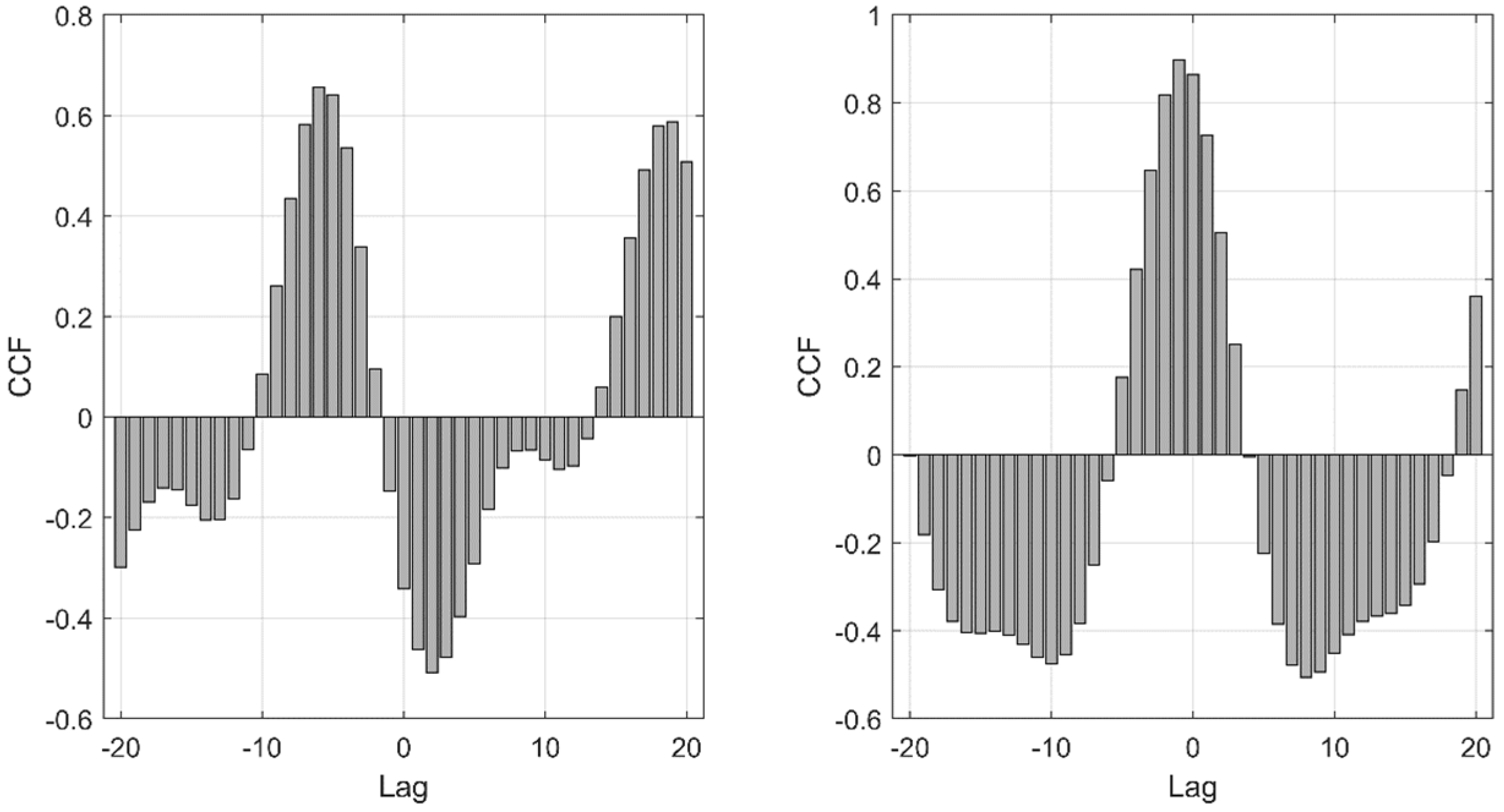
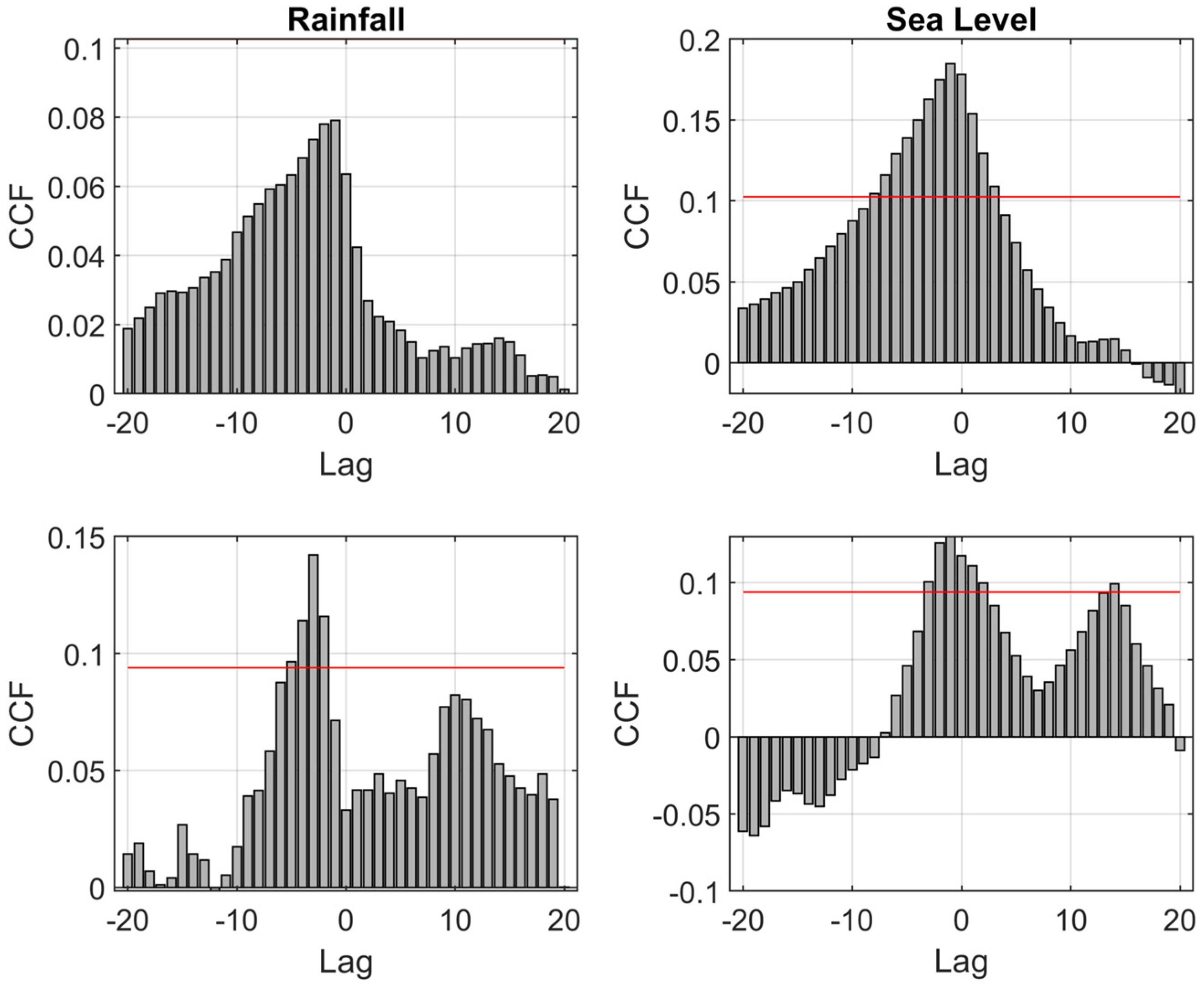
3.3. Auto-Correlation and Cross-Correlation Functions of Daily Data
3.4. Linear Mixed Model for Daily Variation in Levels
4. Discussion
4.1. Statistical Methodologies to Interpret Spring Level Time Series
4.2. Hydrogeological Implications of the Time-Series Analysis Results
5. Conclusions
Author Contributions
Funding
Data Availability Statement
Acknowledgments
Conflicts of Interest
Abbreviations
| AMSL | above mean sea level |
| EC | electrical conductivity |
| CCF | cross-correlation function |
| ACFs | auto-correlation functions |
| PACF | partial auto-correlation function |
| CWT | continuous wavelet transform |
| AIC | Akaike information criterion |
| IRFs | impulse response functions |
| AR | auto-regressive |
| XWT | cross-wavelet transform |
| BLUP | best linear unbiased predictor |
Appendix A. Theory
Appendix A.1. Time-Series Descriptive Statistics
Appendix A.2. Time-Series Analyses in Frequency Domain
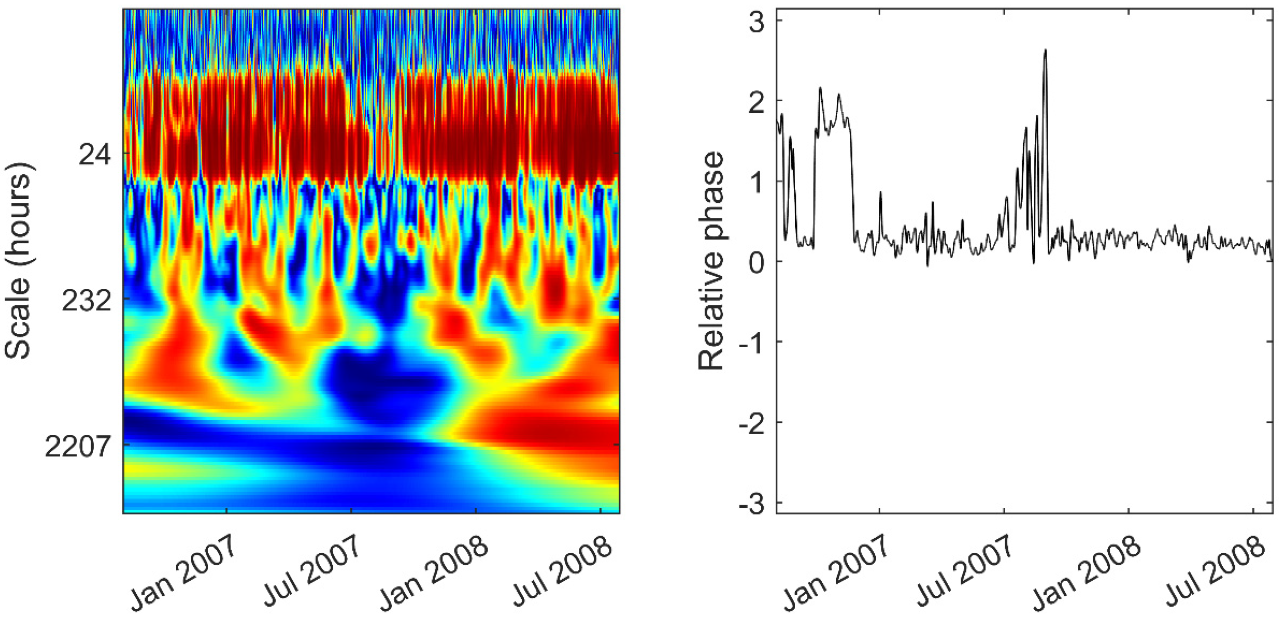
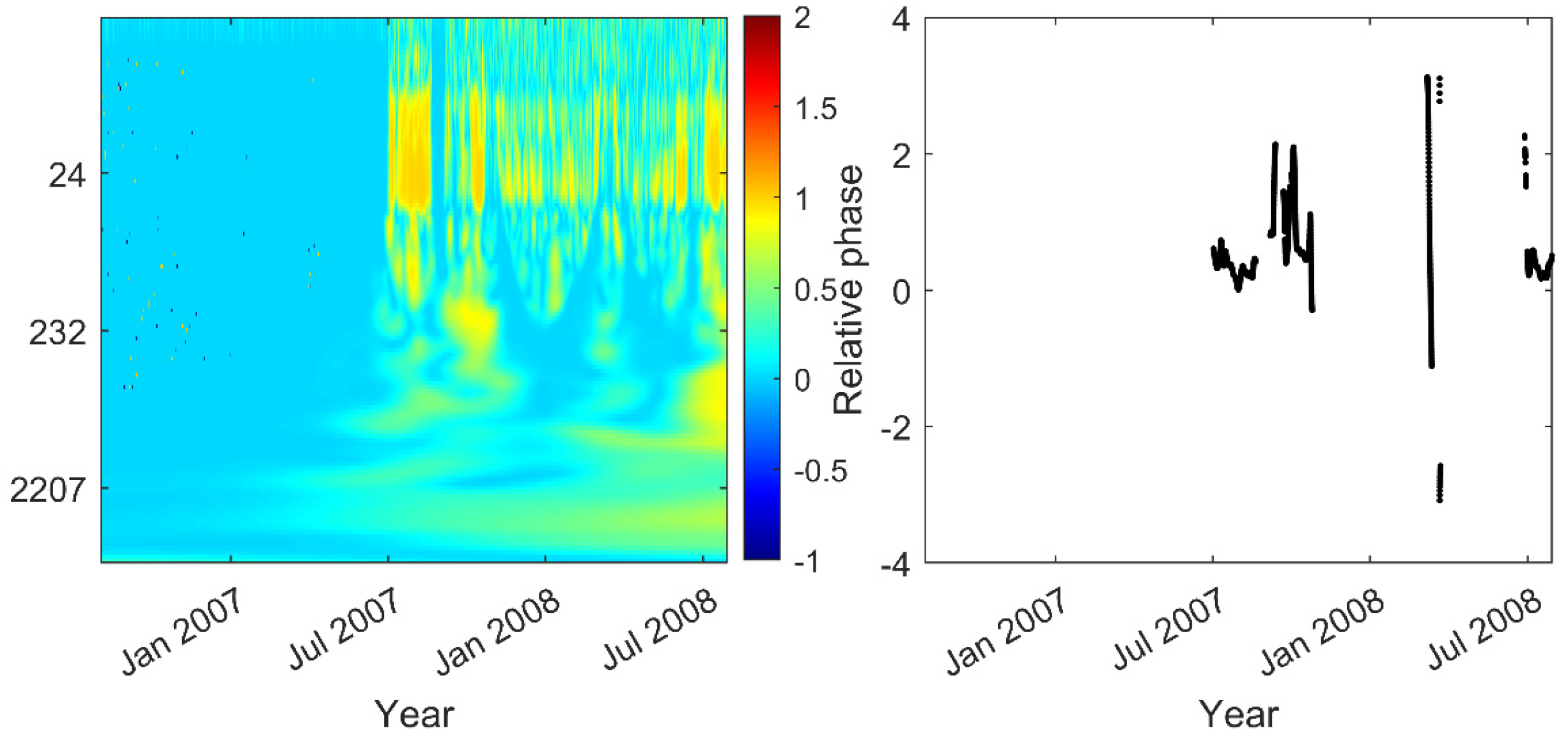
Appendix A.3. Wavelet Analyses for Time-Variant Time Series
Appendix A.4. Time-Series Modelling
References
- Bakalowicz, M. Karst and karst groundwater resources in the Mediterranean. Environ. Earth Sci. 2015, 74, 5–14. [Google Scholar] [CrossRef]
- Bear, J.; Cheng, A.H.D.; Sorek, S.; Ouazar, D.; Herrera, I. (Eds.) Seawater Intrusion in Coastal Aquifers: Concepts, Methods and Practices; Springer Science & Business Media: Berlin/Heidelberg, Germany, 1999; Volume 14. [Google Scholar]
- Gjurašin, K. Prilog Hidrografiji Primorskog Krša (Contribution to the Littoral Karst Hydrography); Tehnicki Vjesnik 59/4-6: Zagreb, Croatia, 1942; pp. 1–6. (In Croatian) [Google Scholar]
- Kuscer, I.; Kuscer, D. Observations on Brackish Karst Sources and Sea Swallow-Holes on the Yugoslav Coast; Mémoires A.I.H.; Réunion d’Athènes: Athènes, Greece, 1964; pp. 344–353. [Google Scholar]
- Fleury, P.; Bakalowicz, M.; de Marsily, G. Submarine springs and coastal karst aquifers: A review. J. Hydrol. 2007, 339, 79–92. [Google Scholar] [CrossRef]
- Chappell, J.; Shackleton, N. Oxygen isotopes and sea level. Nature 1986, 324, 137–140. [Google Scholar] [CrossRef]
- Stroj, A.; Paar, D. Water and air dynamics within a deep vadose zone of a karst massif: Observations from the Lukina jama–Trojama cave system (−1,431 m) in Dinaric karst (Croatia). Hydrol. Process. 2019, 33, 551–561. [Google Scholar] [CrossRef]
- Paar, D.; Mance, D.; Stroj, A.; Pavić, M. Northern Velebit (Croatia) karst hydrological system: Results of a preliminary 2H and 18O stable isotope study. Geol. Croat. 2019, 72, 205–213. [Google Scholar] [CrossRef]
- Bakšić, D.; Paar, D.; Stroj, A.; Lacković, D. Northern Velebit deep caves. In Proceedings of the 16th International Congress of Speleology, Brno, Czech Republic, 21–28 July 2013; Filippi, M., Bosak, P., Eds.; Czech Speleological Society and UIS: Brno, Czech Republic, 2013; Volume 2, pp. 24–29, ISBN 978-80-87857-08-3. [Google Scholar]
- Stroj, A. Underground Water Flows in the Hinterland of the Velebit Channel Coastal Karst Springs. Ph.D. Thesis, University of Zagreb, Zagreb, Republic of Croatia, 2010. [Google Scholar]
- Bonacci, O.; Roje-Bonacci, T. Sea water intrusion in coastal karst springs: Example of the Blaž Spring (Croatia). Hydrol. Sci. J. 1997, 42, 89–100. [Google Scholar] [CrossRef]
- Ploessel, M.R. Ghyben-Herzberg ratio. In Beaches and Coastal Geology; Encyclopedia of Earth Sciences Series; Springer: New York, NY, USA, 1982. [Google Scholar] [CrossRef]
- Biondić, R. Selected Coastal Karst Aquifers (Croatia): Jurjevska Žrnovnica. In The Main Karstic Aquifers of Southern Europe; Calaforra, J.M., Ed.; European Commission, Directorate–General for Research, EUR 20911 (Cost Action 621), EC: Brussels, Belgium, 2004; 123p. [Google Scholar]
- Padilla, A.; Pulido-Bosch, A. Study of hydrographs of karstic aquifers by means of correlation and cross-spectral analysis. J. Hydrol. 1995, 168, 73–89. [Google Scholar] [CrossRef]
- Larocque, M.; Mangin, A.; Razack, R.; Banton, O. Contribution of correlation and spectral analyses to the regional study of a large karst aquifer (Charente, France). J. Hydrol. 1998, 205, 217–231. [Google Scholar] [CrossRef]
- Jukić, D.; Denić-Jukić, V. Partial spectral analysis of hydrological time series. J. Hydrol. 2011, 400, 223–233. [Google Scholar] [CrossRef]
- Jukić, D.; Denić-Jukić, V. Investigating relationships between rainfall and karst-spring discharge by higher-order partial correlation functions. J. Hydrol. 2015, 530, 24–36. [Google Scholar] [CrossRef]
- Charlier, J.-B.; Ladouche, B.; Maréchal, J.-C. Identifying the impact of climate and anthropic pressures on karst aquifers using wavelet analysis. J. Hydrol. 2015, 523, 610–623. [Google Scholar] [CrossRef]
- Massei, N.; Dupont, J.P.; Mahler, B.J.; Laignel, B.; Fournier, M.; Valdes, D.; Ogier, S. Investigating transport properties and turbidity dynamics of a karst aquifer using correlation, spectral and wavelet analyses. J. Hydrol. 2006, 329, 244–257. [Google Scholar] [CrossRef]
- Rezaei, A.; Saatsaz, M. Large-scale climate indices teleconnections with hydrochemical and isotopic characteristics of a karst spring using wavelet analysis. Environ. Earth Sci. 2021, 80, 335. [Google Scholar] [CrossRef]
- Wu, L.; Wang, S.; Bai, X.; Chen, F.; Li, C.; Ran, C.; Zhang, S. Identifying the Multi-Scale Influences of Climate Factors on Runoff Changes in a Typical Karst Watershed Using Wavelet Analysis. Land 2022, 11, 1284. [Google Scholar] [CrossRef]
- Zhang, J.; Zhu, Z.; Hao, H. The Effects of Climate Variation and Anthropogenic Activity on Karst Spring Discharge Based on the Wavelet Coherence Analysis and the Multivariate Statistical. Sustainability 2023, 15, 8798. [Google Scholar] [CrossRef]
- Çeliker, M.; Uzun, S.; Yıldırım, G. Periodic variations of karstic spring discharge and precipitation from the perspective of wavelet analysis techniques: A case study of tacin spring (Kayseri, Türkiye). Environ. Earth Sci. 2025, 84, 46. [Google Scholar] [CrossRef]
- Lovrinović, I.; Srzić, V.; Matić, I.; Brkić, M. Combined Multilevel Monitoring and Wavelet Transform Analysis Approach for the Inspection of Ground and Surface Water Dynamics in Shallow Coastal Aquifer. Water 2022, 14, 656. [Google Scholar] [CrossRef]
- Treviño, J.; Rodríguez-Rodríguez, M.; Montes-Vega, M.J.; Aguilera, H.; Fernández-Ayuso, A.; Fernández-Naranjo, N. Wavelet Analysis on Groundwater, Surface-Water Levels and Water Temperature in Doñana National Park (Coastal Aquifer in Southwestern Spain). Water 2023, 15, 796. [Google Scholar] [CrossRef]
- Yang, G.; McCoy, K. Modeling groundwater-level responses to multiple stresses using transfer-function models and wavelet analysis in a coastal aquifer system. J. Hydrol. 2023, 627, 130426. [Google Scholar] [CrossRef]
- Akaike, H. Information theory and the maximum likelihood principle in 2nd International Symposium on Information Theory. In Proceedings of the 2nd International Symposium on Information Theory; Petrov, B.N., Csäki, F., Eds.; Akademiai Kiàdo: Budapest, Hungary, 1973. [Google Scholar]
- Mallat, J. A Wavelet Tour of Signal Processing; Academic Press: New York, NY, USA, 1999. [Google Scholar]
- Ferris, J.; Branch, G.S.G.W. Cyclic Fluctuations of Water Level as a Basis for Determining Aquifer Transmissibility; US Dept. of the Interior, Geological Survey. Water Resources Division, Ground Water Branch: Washington, DC, USA, 1952. [CrossRef]
- Merritt, M.L. Estimating Hydraulic Properties of the Floridan Aquifer System by Analysis of Earth-Tide, Ocean-Tide, and Barometric Effects, Collier and Hendry Counties, Florida; US Department of the Interior, US Geological Survey: Reston, VA, USA, 2004; No. 3. [CrossRef]
- Perriquet, M.; Leonardi, V.; Henry, T.; Jourde, H. Saltwater wedge variation in a non-anthropogenic coastal karst aquifer influenced by a strong tidal range (Burren, Ireland). J. Hydrol. 2014, 519, 2350–2365. [Google Scholar] [CrossRef]
- Zhang, H. Characterization of a multi-layer karst aquifer through analysis of tidal fluctuation. J. Hydrol. 2021, 601, 126677. [Google Scholar] [CrossRef]
- Ghyben, B.W. Nota in verband met de voorgenomen put boring nabij, Amsterdam Kononkl. Inst. Ing. Tijdschr. 1889, 1888–1889, 8–22. [Google Scholar]
- Herzberg, B. Die Wasserversorgung einiger Nordseebäder. J. Gasbeleucht. Wasserversorg. 1901, 44, 815–844. [Google Scholar]
- Williams, P.W. The role of the epikarst in karst and cave hydrogeology: A review. Int. J. Speleol. 2008, 37, 1–10. [Google Scholar] [CrossRef]
- Jones, W.K. Physical structure of the epikarst. Acta Carsologica 2013, 42, 311–314. [Google Scholar] [CrossRef]
- Stroj, A.; Briški, M.; Oštrić, M. Study of Groundwater Flow Properties in a Karst System by Coupled Analysis of Diverse Environmental Tracers and Discharge Dynamics. Water 2020, 12, 2442. [Google Scholar] [CrossRef]
- Diggle, P.J. Time Series: A Biostatistical Introduction; Oxford Science Publications: Oxford, UK, 1990. [Google Scholar] [CrossRef]
- Durbin, J. The fitting of time series models. ISI 1960, 28, 233–244. [Google Scholar] [CrossRef]
- Bracewell, R.N. The Fourier Transform and Its Applications; McGraw-Hill: New York, NY, USA, 1986. [Google Scholar] [CrossRef]
- Cooley, J.W.; Tukey, J.W. An algorithm for the machine calculation of complex Fourier series. Math. Comput. 1965, 19, 297–301. [Google Scholar] [CrossRef]
- Torrence, C.; Compo, G.P. A practical guide to wavelet analysis. Bull. Am. Meteorol. Soc. 1998, 79, 61–78. [Google Scholar] [CrossRef]
- Hipel, K.W.; McLeod, A.I. Time Series Modelling of Water Resources and Environmental Systems; Elsevier: Amsterdam, The Netherlands, 1994. [Google Scholar]
- Marchant, B.; Mackay, J.; Bloomfield, J. Quantifying uncertainty in predictions of groundwater levels using formal likelihood methods. J. Hydrol. 2016, 540, 699–711. [Google Scholar] [CrossRef]
- Webster, R.; Oliver, M.A. Geostatistics for Environmental Scientists; John Wiley & Sons: Chichester, UK, 2007. [Google Scholar] [CrossRef]
- Lark, R.M.; Cullis, B.R.; Welham, S.J. On spatial prediction of soil properties in the presence of a spatial trend: The empirical best linear unbiased predictor (E-BLUP) with REML. Eur. J. Soil Sci. 2006, 57, 787–799. [Google Scholar] [CrossRef]


| Spring | Fixed Effects | AIC | Bias m | Variance Explained % | Mean SSE | Variance Explained by Fixed Effects % |
|---|---|---|---|---|---|---|
| 1 | C | 218.54 | 0.00 | 95 | 0.86 | 0 |
| 1 | C+R | 157.06 | 0.00 | 96 | 0.96 | 49 |
| 1 | C+R+Sea | 110.71 | 0.00 | 96 | 1.00 | 59 |
| 1 | C+R+Sea+Seas | 104.52 | 0.00 | 96 | 1.00 | 70 |
| 2 | C | 292.05 | 0.00 | 96 | 0.75 | 0 |
| 2 | C+R | 257.72 | 0.00 | 96 | 0.81 | 17 |
| 2 | C+R+Sea | 243.82 | 0.00 | 96 | 0.81 | 17 |
| 2 | C+R+Sea+Seas | 219.51 | 0.00 | 96 | 0.78 | 69 |
Disclaimer/Publisher’s Note: The statements, opinions and data contained in all publications are solely those of the individual author(s) and contributor(s) and not of MDPI and/or the editor(s). MDPI and/or the editor(s) disclaim responsibility for any injury to people or property resulting from any ideas, methods, instructions or products referred to in the content. |
© 2025 by the authors. Licensee MDPI, Basel, Switzerland. This article is an open access article distributed under the terms and conditions of the Creative Commons Attribution (CC BY) license (https://creativecommons.org/licenses/by/4.0/).
Share and Cite
Stroj, A.; Lukač Reberski, J.; Maurice, L.D.; Marchant, B.P. Time-Series Analysis of Monitoring Data from Springs to Assess the Hydrodynamic Characteristics of a Coastal Discharge Zone: Example of Jurjevska Žrnovnica Springs in Croatia. Hydrology 2025, 12, 118. https://doi.org/10.3390/hydrology12050118
Stroj A, Lukač Reberski J, Maurice LD, Marchant BP. Time-Series Analysis of Monitoring Data from Springs to Assess the Hydrodynamic Characteristics of a Coastal Discharge Zone: Example of Jurjevska Žrnovnica Springs in Croatia. Hydrology. 2025; 12(5):118. https://doi.org/10.3390/hydrology12050118
Chicago/Turabian StyleStroj, Andrej, Jasmina Lukač Reberski, Louise D. Maurice, and Ben P. Marchant. 2025. "Time-Series Analysis of Monitoring Data from Springs to Assess the Hydrodynamic Characteristics of a Coastal Discharge Zone: Example of Jurjevska Žrnovnica Springs in Croatia" Hydrology 12, no. 5: 118. https://doi.org/10.3390/hydrology12050118
APA StyleStroj, A., Lukač Reberski, J., Maurice, L. D., & Marchant, B. P. (2025). Time-Series Analysis of Monitoring Data from Springs to Assess the Hydrodynamic Characteristics of a Coastal Discharge Zone: Example of Jurjevska Žrnovnica Springs in Croatia. Hydrology, 12(5), 118. https://doi.org/10.3390/hydrology12050118