Glacier, Wetland, and Lagoon Dynamics in the Barroso Mountain Range, Atacama Desert: Past Trends and Future Projections Using CA-Markov

Abstract

Glacial retreat is a major global challenge, particularly in arid and semi-arid regions where glaciers serve as critical water sources. This research focuses on glacial retreat and its impact on land cover and land use changes (LULC) in the Barroso Mountain range, Tacna, Peru, which is a critical area for water resources in the hyperarid Atacama Desert. Employing advanced remote sensing techniques through the Google Earth Engine (GEE) cloud computing platform, we analyzed historical trends (1985–2022) using Landsat satellite imagery. A normalized index classification was carried out to generate LULC maps for the years 1986, 2001, 2012, and 2022. Future projections until 2042 were developed using Cellular Automata–Markov (CA–Markov) modeling in QGIS, incorporating six predictive environmental variables. The resulting maps presented an overall accuracy (OA) greater than 83%. Historical analysis revealed a dramatic glacier reduction from 44.7 km² in 1986 to 7.4 km² in 2022. In contrast, wetlands expanded substantially from 5.70 km² to 12.14 km², indicating ecosystem shifts potentially driven by glacier meltwater availability. CA–Markov chain modeling projected further glacier loss to 3.07 km² by 2042, while wetlands are expected to expand to 18.8 km² and bodies of water will reach 4.63 km². These future projections (with accuracies above 84%) underline urgent implications for water management, environmental sustainability, and climate adaptation strategies, particularly with regard to downstream hydrological risks and ecosystem resilience.

1. Introduction

Over the past century, glaciers around the world have retreated at an unprecedented rate, threatening freshwater supplies in many arid and semi-arid regions. The Barroso mountain range, located within the hyperarid Atacama Desert, is experiencing rapid glacier loss with potential consequences for wetlands, water resources, and local communities. However, limited research has been conducted to quantify these changes and predict future trends. This study addresses this gap by integrating multi-temporal remote sensing analysis with predictive modeling to assess the impacts of glacial retreat on land use and hydrology in the region.

The Atacama Desert, in northern Chile, is a hyperarid non-polar coastal region almost 1000 km long located in South America [1]. Paleoclimatic records from the region are rare and mostly discontinuous, primarily capturing runoff from the eastern Precordillera rather than local precipitation [2]. Despite these extreme conditions, desert plants have evolved to survive in this environment [3]. However, changes in hydrological processes, including glacier retreat and groundwater depletion, may impact water availability and ecosystem resilience in this fragile landscape.

The Barroso mountain range, located in southern Peru and northern Chile, exhibits climatic conditions consistent with a hyperarid environment, with significant precipitation fluctuations between summer and winter [4,5]. In addition, groundwater plays a crucial role in sustaining various water-dependent sectors, but overexploitation and marine intrusion threaten the sustainability of key aquifers, such as the Caplina coastal aquifer [6,7]. Over the past century, this aquifer has been severely exploited, resulting in increasing salinization and minimal recharge, with fossil water now being the primary source of extraction [8]. The continued retreat of glaciers in the region may further reduce groundwater recharge, exacerbating water scarcity concerns. As glaciers shrink, meltwater contributes to the expansion of Wetlands (high-altitude wetlands). However, as glacier volume continues to decline, the long-term sustainability of these wetlands remains uncertain.

Wetlands are vital buffers in hydrological systems, regulating water flow and supporting biodiversity. In the Barroso region, glacial meltwater has historically contributed to the expansion of Wetlands (high-altitude wetlands). However, as glaciers continue to retreat, the balance between meltwater supply and wetland persistence is changing, with potential consequences for water retention and local biodiversity [9]. The wetlands and salt flats of the Atacama Desert were once freshwater lakes and shallow wet areas during the last glacial period [10]. The formation of salt crusts, primarily from groundwater evaporation, has given rise to dynamic halite layers, which help regulate humidity variations [10,11]. The continental salt flats of the Miocene are scattered in the Central Valley of the Atacama Desert, one of the driest areas on the planet. While some of these salt flats remain hydrologically inactive [10], high-altitude wetlands in the Barroso mountain range continue to play a crucial role in water retention and biodiversity conservation. However, glacial retreat may alter the balance between meltwater supply and wetland persistence, leading to uncertain future dynamics.

Traditional approaches to modeling glacier and wetland changes have been limited by data availability and computational constraints. The integration of Google Earth Engine (GEE) and the Ca–Markov model provides a robust framework for analyzing historical trends and forecasting future changes with high spatial and temporal resolution. Ca–Markov is a combined cellular automata/Markov chain/multicriteria/multiobjective land allocation (MOLA) LULC prediction procedure that adds an element of spatial contiguity as well as a knowledge base of the likely spatial distribution of transitions to the Markov chain analysis [12,13]. This method has been successfully applied to forecast wetland evolution over time [9], and to optimize the classification of multi-temporal land cover changes in various ecosystems [14]. Likewise, it is possible to use the integration of remote sensing data and the Ca–Markov model to analyze the dynamics of land use change and its future prediction [12,13].

In recent years, the availability, accessibility, and temporal and spatial continuity of satellite data (such as Landsat and Sentinel) [15,16,17] and the development of cloud computing platforms, such as Google Earth Engine (GEE) [18], have created an opportunity to map the historical evolution of land cover change, such as bodies of water and glaciers [19].

The implementation of advanced time series analysis methods and dynamic predictive models, combined with satellite data, significantly improves the accuracy of glacial retreat projections. This, in turn, allows for a better understanding of spatial patterns of change and contributes to more effective environmental management and water resource planning in the face of climate change. The impacts of these changes extend across the entire basin and are particularly evident in the lower reaches, such as the Seco River ravine in Tacna, Peru, a region located at the northern edge of the hyperarid core of the Atacama Desert.

This study aims to analyze the historical changes in glacier extent, wetlands, and lagoons in the Barroso mountain range from 1985 to 2022 using satellite imagery. Additionally, it seeks to predict future land cover transformations up to 2042 through the application of the Ca–Markov model. Furthermore, the research evaluates the hydrological implications of these landscape changes, with a particular focus on their impact on discharges in the Seco River ravine near Tacna, Peru. By addressing these objectives, this study provides critical insights for water resource management, climate adaptation strategies, and the preservation of fragile ecosystems in this hyperarid Andean region.

2. Materials and Methods

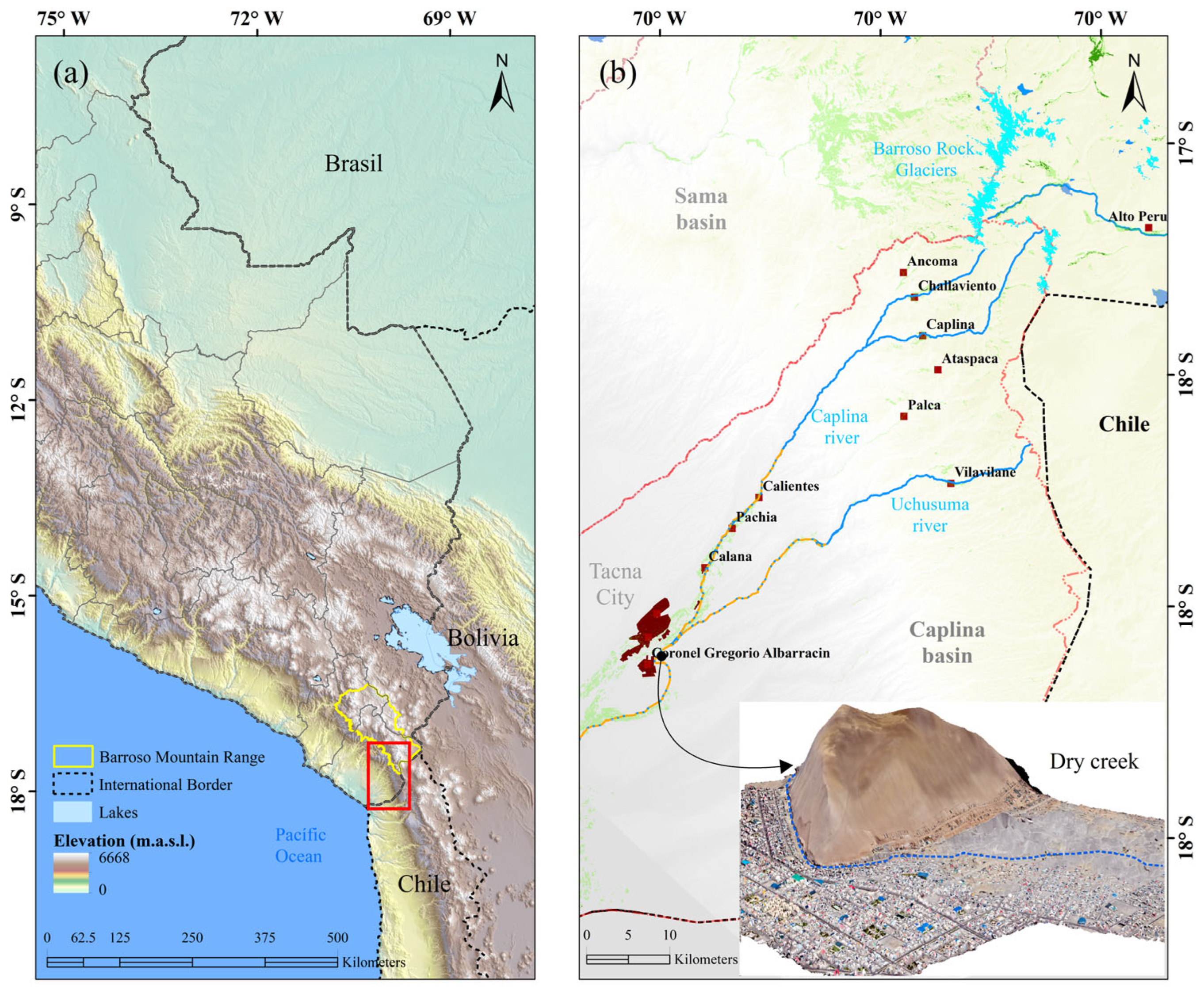
2.1. The Study Area

The study area is located at the headwaters of the Caplina River, covering altitudes from 500 to 4600 m above sea level. The climate is classified as semi-arid to hyperarid, with an average temperature range from 18.1 °C to 13.4 °C and extreme values reaching −15 °C in winter months. Annual precipitation averages 360 mm, with 78% of rainfall occurring between December and March (Figure 1). Hydrologically, the region is dominated by glacial melt contributions to the Caplina River, which serves as a major freshwater source for Tacna, Peru. However, glacial retreat in the Barroso Mountain range has significantly altered recharge processes, contributing to increasing water scarcity and wetland expansion. These dynamics highlight the critical need for predictive modeling of land cover changes in the region. Figure 2 shows the location of the study area; it is also located on the northern edge of the hyperarid core of the Atacama Desert.

2.2. Selection of Satellite Images

The main material used in this study consists of images from the LANDSAT-5 TM and LANDSAT-8 OLI software, with Landsat sensors: Thematic Mapper (TM) and Operational Land Imager (OLI) [20]. On board the Landsat 5 and Landsat 8 satellites, the image collections used were accessed through the GEE platform [18] “https://earthengine.google.com (accessed on 22 January 2025), respectively, they cover the multi-year analysis periods from 1985 to 2022 (

Table 1. Imágenes de reflectancia TOA del programa Landsat.

Collection	Sensor	Periods
LANDSAT/LT05/C02/T1_TOA	TM	1984-03–2012-05
LANDSAT/LE07/C02/T1_TOA	ETM+	1999-05–2022-04
LANDSAT/LC08/C02/T1_TOA	OLI/TIRS	2013-03–present

).

The top-of-the-atmosphere (TOA) images available in the GEE catalog were used to collect data, which offers access to a vast amount of preprocessed satellite images. These TOA images are ideal for reflectance analysis studies, as they provide radiation reflected by the Earth’s surface without interference from the atmosphere [21] with orthorectification and a spatial resolution of 30 m in the spectral bands [22].

The selection of satellite images was based on data availability, cloud cover constraints, and key hydrological periods identified in the study area. The years were chosen to capture multi-decadal trends in glacial retreat and wetland expansion. The Landsat TOA reflectance product was selected due to its pre-processing advantages and radiometric consistency across multiple sensors. However, potential limitations, such as seasonal cloud contamination and spectral mixing in mountainous terrain, were accounted for using cloud-masking algorithms and visual inspections.

2.3. Cloud-Based Processing

This study used the free cloud computing platform Google Earth Engine (GEE). GEE is a cloud-based tool designed for geospatial analysis on a planetary scale [18]. The processing power of Google’s supercomputer is used to address problems of global relevance [23]. This platform provides online access to quickly and efficiently pre-processed data, available through the Google Earth Engine API. It also uses client libraries in programming languages, such as JavaScript ECMAScript 6.0 and Python 3.13.2, to facilitate the analysis and visualization of geospatial data [24].

The data processing included the selection of Landsat scenes (TM and OLI) available in GEE, corresponding to the period of Julian days 135 to 227, which covers the dry season in the study area. Then, an algorithm was applied to obtain an image without clouds or shadows. Subsequently, normalized indices were used for analysis. Finally, the types of land cover (glaciers, lakes, and wetlands) were identified using thresholds in the indices Table …… Results of glacier surface, wetlands and bodies of water in (km²) in the Barroso mountain range to calculate the surface extensions of the last 37 years. 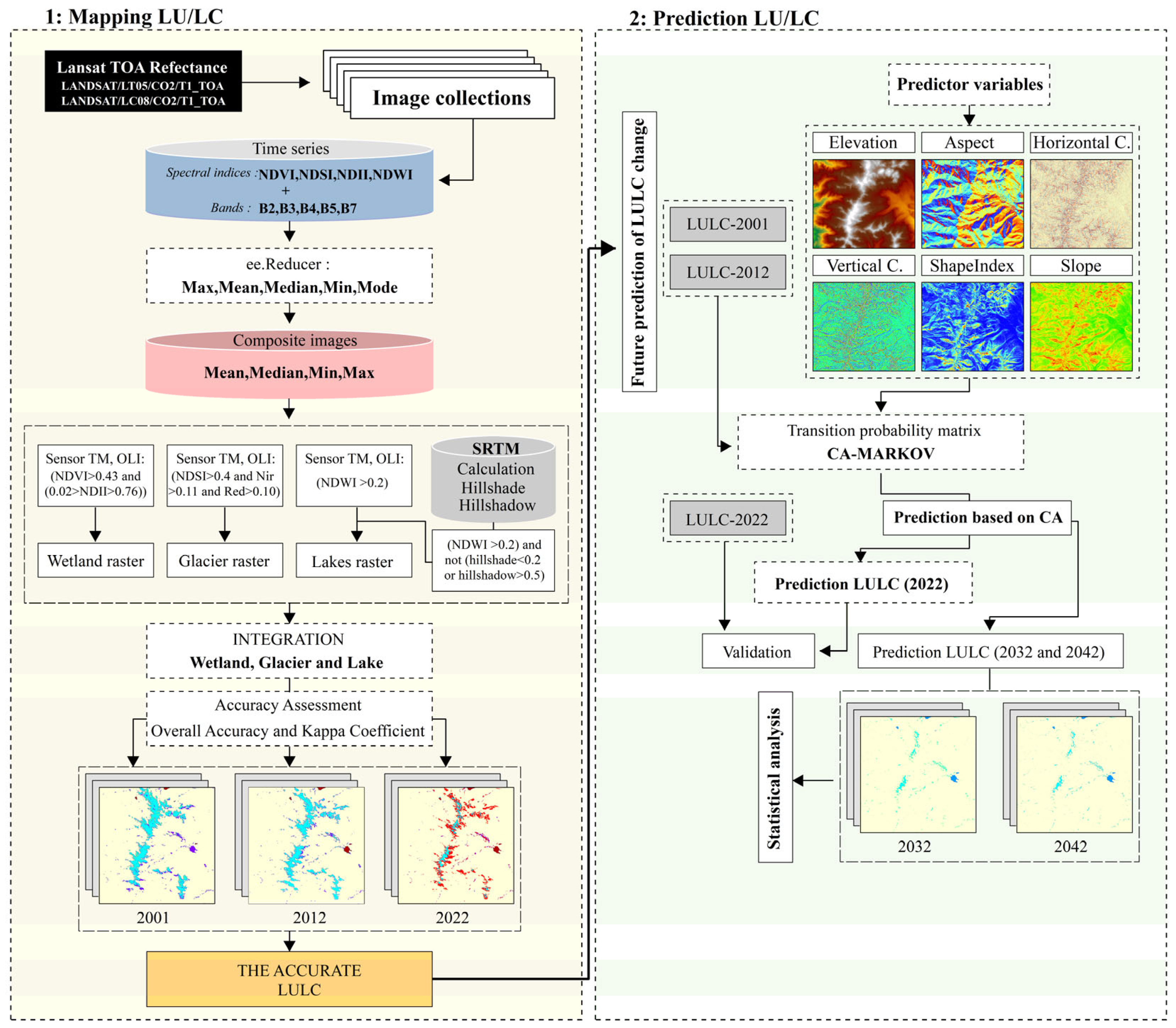Figure 3 shows the methodological diagram of this work.

2.4. Image Collection Reduction

To simplify the collection of images (Image Collection), the imageCollection.reduce() tool in GEE was used; this allowed for transforming the collection of images into a single one. In particular, the calculation is performed at the pixel level, so that each pixel in the resulting image reflects the median value of all images corresponding to the selected period and location within the collection [19].

2.5. Glacier Identification

The methodology used consists of 5 processes: (1) selection and masking of clouds in satellite images, (2) calculation of the Normalized Difference Snow Index (NDSI), (3) generation of annual Landsat mosaics, (4) annual classification of glaciers, and (5) evaluation of the model accuracy.

This work is focused on glacial surfaces that are mostly clean or only slightly contaminated. Glaciers covered by debris have an extremely low representativeness, representing approximately 5.4% of the total glacial areas in tropical regions [25].

Glacier extent was classified using the Normalized Difference Snow Index (NDSI) with an empirically determined threshold of 0.20, based on historical spectral profiles of glacier surfaces in the study region. Since debris-covered glaciers may lead to classification errors, visual inspections and manual corrections were applied to reduce false positives. The wetland classification method integrated NDVI (threshold > 0.43) and NDII (0.02 < NDII < 0.76), leveraging elevation data (SRTM DEM > 3700 m) to refine wetland boundaries.

2.6. Normalized Difference Snow Index

The normalized difference snow index (NDSI) is used to identify snow in comparison to other cover characteristics and estimate the area covered by snow in satellite images [26]. In this way, it can also be used to identify glacial coverage. The NDSI was previously calculated sectioned and masked, the expression of the equation is as follows:

$$NDSI={\displaystyle \frac{\left(GREEN-SWIR\right)}{\left(GREEN+SWIR\right)}},$$

(1)

where GREEN is the reflectance of the green band and SWIR is the reflectance of the shortwave infrared band. To classify annual glaciers, an empirical decision tree with thresholds α, β, and γ was used that has varied depending on the year and type of sensor (TM and OLI), with average values of the thresholds α = 0.20 β = 0.11, and γ = 0.10, respectively. The thresholds have been adjusted with visual monitoring of the classification and year [19].

2.7. Lagoon Identification

Lagoon identification is an NDWI-based extraction method that completely and accurately extracts water from remote sensing images with superior performance compared to other methods [27], offering a more accurate assessment of water availability [28]. The NDWI index was previously calculated, sectioned, and masked. The expression of the equation is as follows:

$${\mathrm{N}\mathrm{D}\mathrm{W}\mathrm{I}}_{\left(\mathrm{M}\mathrm{c}\mathrm{F}\mathrm{e}\mathrm{e}\mathrm{t}\mathrm{e}\mathrm{r}\mathrm{s}\right)} ={\displaystyle \frac{\left(\mathrm{G}\mathrm{R}\mathrm{E}\mathrm{E}\mathrm{N}-\mathrm{N}\mathrm{I}\mathrm{R}\right)}{\left(\mathrm{G}\mathrm{R}\mathrm{E}\mathrm{E}\mathrm{N}+\mathrm{N}\mathrm{I}\mathrm{R}\right)}}.$$

(2)

The Western mountain range generates shadows in satellite images due to its mountainous terrain and low solar angles, especially outside of summer. Terrain modeling was used to identify areas in Landsat scenes affected by shadows, which complicate the detection of water bodies in the NDWI index.

Digital elevation models (DEM) are essential to calculate the angle of solar incidence and the shadow produced by the relief [29]. In this analysis, the DEM SRTM (Shuttle Radar Topography Mission) was used with a resolution of 1 arc second, available on the GEE platform with the ID (USGS/SRTMGL1_003) [30]. The angle of solar incidence is determined using the following equation [31].

$$\mathrm{i}=\mathrm{a}\mathrm{r}\mathrm{c}\mathrm{o}\mathrm{s}\left(\cos \left(\mathsf{\theta }\right)\cos \left(\mathrm{e}\right)+\sin \left(\mathsf{\theta }\right)\mathrm{s}\mathrm{i}\mathrm{n}\left(\mathrm{e}\right)\cos \left(\phi \mathrm{m}-\phi \mathrm{s}\right)\right),$$

(3)

where i represents the angle of solar incidence, θ is the solar zenith angle, e is the inclination, φm aspect, and φs solar azimuth.

The algorithm for calculating the shading value is described in the following equation:

$$\mathrm{H}\mathrm{i}\mathrm{l}\mathrm{l}\mathrm{s}\mathrm{h}\mathrm{a}\mathrm{d}\mathrm{e}=\mathrm{c}\mathrm{o}\mathrm{s}\left(\mathsf{\theta }\right)\mathrm{c}\mathrm{o}\mathrm{s}\left(\mathrm{e}\right)+\mathrm{s}\mathrm{i}\mathrm{n}\left(\mathsf{\theta }\right) \mathrm{\ast }\sin \left(\mathrm{e}\right) \mathrm{\ast } \mathrm{c}\mathrm{o}\mathrm{s}\left(\phi \mathrm{m}-\phi \mathrm{s}\right).$$

(4)

On the GEE platform, the Hillshade was calculated using the “ee.Terrain.hillshade” tool, and the HillShadow was calculated using the “ee.Algorithms.HillShadow” tool. To obtain a shadow map for each period of the year and each collection of images, the minimum values calculated in the Hillshade and the maximum values of the HillShadow were combined.

To obtain the lake raster, the NDWI index was classified with the threshold (NDWI > 0.2) and, in order not to be confused with mountain shadow, additional restrictions were applied (hillShade < 0.2 or hillShadow > 0.5) [32].

2.8. Identification of Wetlands

The classification of the wetlands was carried out using two normalized indices. NDVI is used to map and monitor wetlands and to classify contents within wetland boundaries [33,34,35]. The second normalized difference infrared index, NDII, was used to identify soil moisture and vegetation, allowing a more precise evaluation of wet and dry areas within wetlands (

Table 2. Normalized spectral indices used for the classification of wetlands.

Index	Formula	Reference
Normalized Difference Vegetation Index	$\mathrm{N}\mathrm{D}\mathrm{V}\mathrm{I}={\displaystyle \frac{(\mathrm{N}\mathrm{I}\mathrm{R}-\mathrm{R}\mathrm{E}\mathrm{D})}{(\mathrm{N}\mathrm{I}\mathrm{R}+\mathrm{R}\mathrm{E}\mathrm{D})}}$	[39]
Infrared Normalized Difference Index	$\mathrm{N}\mathrm{D}\mathrm{I}\mathrm{I}={\displaystyle \frac{(\mathrm{N}\mathrm{I}\mathrm{R}-\mathrm{S}\mathrm{W}\mathrm{I}\mathrm{R})}{(\mathrm{N}\mathrm{I}\mathrm{R}+\mathrm{S}\mathrm{W}\mathrm{I}\mathrm{R})}}$	[40]

) [36,37,38].

In addition to the NDVI and NDII indices, wetland classification was refined using elevation, land cover, and slope data. The digital elevation model SRTM was used to obtain information on altitude, considering areas located above 3700 m above sea level. To obtain the wetland raster, two indices were classified, namely NDVI and NDII with the conditional (and) and with the following thresholds: (NDVI > 0.43) and (0.02 < NDII < 0.76) [41].

3. Results

3.1. Regression Analysis on Coverage Influenced by Glaciers

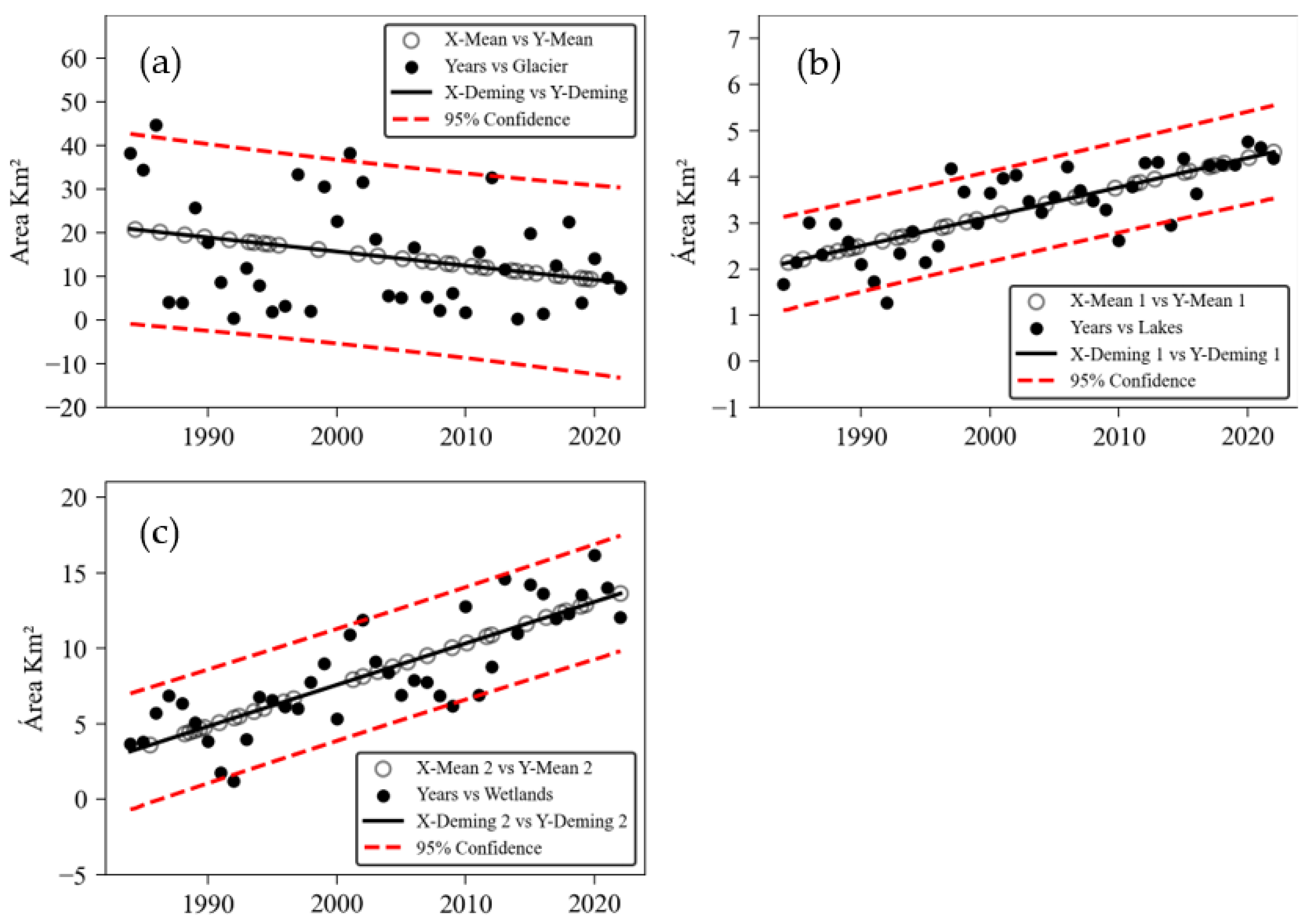
Figure 4 shows the variation in different area-related variables over time in glaciers, lakes, and wetlands. Regression lines help visualize the data’s trend, while 95% confidence bands indicate the variability and certainty of these trends. The data show a negative trend in glaciers and a positive trend in wetlands and lagoons of glacial origin.

Table 3. Results of glacier surface, wetlands, and bodies of water (in km²) in the Barroso mountain range.

Año	Glacier	Variation	Wetland	Variation	Lagoon	Variation
1984	38,149		3650		1667
1985	34,467	−3682	3795	0.146	2143	0.476
1986	44,642	10,175	5700	1904	3013	0.870
1987	4103	−40,539	6849	1149	2317	−0.696
1988	4011	−0.092	6343	−0.506	2979	0.662
1989	25,749	21,738	5052	−1291	2592	−0.387
1990	17,817	−7932	3848	−1205	2109	−0.483
1991	8725	−9092	1773	−2074	1727	−0.382
1992	0.472	−8253	1188	−0.585	1269	−0.457
1993	11,938	11,467	3972	2784	2340	1.070
1994	7935	−4003	6777	2805	2808	0.468
1995	1912	−6023	6548	−0.230	2151	−0.657
1996	3312	1399	6154	−0.393	2510	0.359
1997	33,340	30,028	6004	−0.150	4180	1670
1998	2027	−31,312	7751	1748	3681	−0.499
1999	30,536	28,508	8974	1223	2997	−0.684
2000	22,592	−7943	5337	−3638	3646	0.649
2001	38,272	15,680	10,879	5543	3970	0.324
2002	31,558	−6714	11,878	0.999	4033	0.063
2003	18,504	−13,054	9106	−2772	3468	−0.565
2004	5613	−12,891	8407	−0.699	3232	−0.236
2005	5119	−0.494	6886	−1521	3572	0.340
2006	16,582	11,463	7862	0.976	4214	0.642
2007	5368	−11,215	7742	−0.120	3710	−0.504
2008	2255	−3113	6853	−0.889	3487	−0.223
2009	6125	3870	6173	−0.680	3288	−0.199
2010	1861	−4264	12,771	6599	2625	−0.663
2011	15,552	13,691	6901	−5871	3785	1160
2012	32,631	17,080	8759	1859	4301	0.516
2013	11,561	−21,070	14,609	5849	4315	0.014
2014	0.253	−11,308	10,974	−3635	2959	−1356
2015	19,884	19,631	14,216	3242	4399	1440
2016	1515	−18,369	13,601	−0.616	3629	−0.770
2017	12,576	11,061	11,962	−1638	4247	0.618
2018	22,482	9905	12,309	0.346	4267	0.020
2019	3953	−18,529	13,538	1229	4263	−0.004
2020	14,114	10,161	16,157	2619	4756	0.493
2021	9666	−4448	14,019	−2138	4635	−0.121
2022	7413	−2253	12,067	−1953	4394	−0.241
Mean		−0.809		0.2215		0.0718

and Figure 5 show the area covered by glaciers, with a complex polynomial trend indicating variations in the surface over time. From the fluctuations and shape of the curve, there were periods of decrease and increase in the glacier surface, but it maintained a negative trend.

A fluctuating trend is observed in the surface of the lakes with a slight decrease in some periods, but the positive trend remains. In the wetlands, it is similar to the glaciers, and the wetlands also show considerable variability in their area over time, maintaining a positive trend.

Multi-temporal studies carried out by other researchers in the Cordillera Blanca, Peru, indicate that the reduction in glaciers contributes to the increased water level in the wetlands, which could be generating their expansion [42]. It could be stated that there is an inverse correlation between glacial retreat and the increase in wetland coverage.

The observed fluctuations in glacier surface (Figure 4) suggest that glacial retreat is not linear but responds to interannual climate variability. For example, years with increased glacier surface (1989, 1997, 2012) may be linked to anomalous precipitation or cold periods, whereas rapid declines (2001, 2016) align with warm phases or droughts. Studies in the Cordillera Blanca, Peru, have shown similar patterns, where ENSO phases significantly influence glacial mass balance [42]. Further investigation into temperature trends, precipitation shifts, and glacier mass balance records is recommended.

3.2. Historical Transformation of Glacial Cover, Lakes and Wetlands

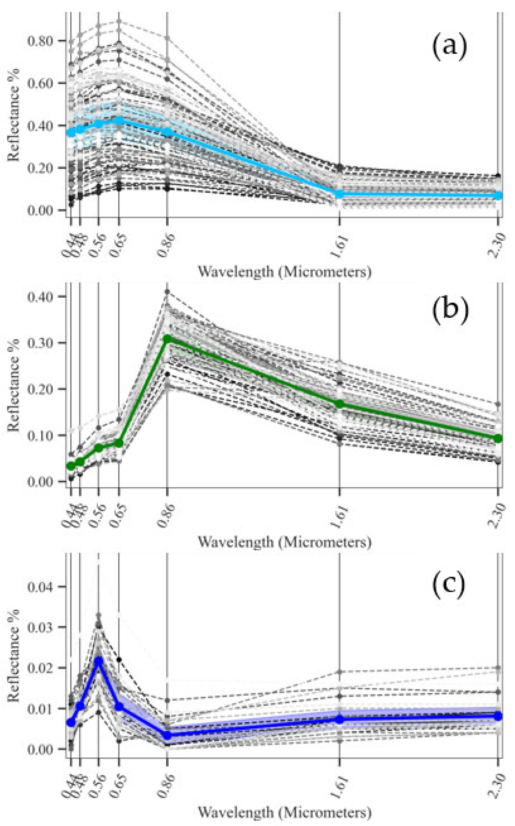
In the work process, 250 points were selected randomly within the layers corresponding to glaciers, wetlands, and lakes, to extract the reflectance associated with each type of coverage. Subsequently, spectral profile graphs were generated to analyze and contrast the quality of the pixels in each coverage.

Figure 5 shows the relationship between reflectance (%) and wavelength in micrometers (μm) of the glacier, wetlands, and lake, highlighting how this varies under different conditions or scenarios. In case (a) glaciers, a reflectance peak is observed in the range of the visible spectrum (approximately between 0.45 and 0.67 μm), characteristic of clean and pure ice. In case (b), the vegetation of the wetland cover, in the visible range (0.45–0.67 μm) the reflectance is low due to the absorption of light by the pigments, mainly chlorophyll [42,43]. At the green peak, approximately 0.56 μm the vegetation reflects more light in the green band, which gives it its characteristic color. In case (c), the spectral signature of water is shown, characterized by a reflectance peak at 0.55 µm due to light scattering, followed by a decrease between 0.65 and 0.86 µm due to high absorption in the red and near-infrared. At SWIR 1.6 and 2.3 µm, the reflectance is almost zero due to the extreme absorption of water.

Overall, the observed expansion of wetlands (Figure 6) suggests that glacial meltwater contributes directly to their growth. However, the exact hydrological mechanism remains uncertain. Possible explanations include increased meltwater runoff recharging high-altitude wetlands or a shift in the groundwater balance that favors wetland persistence. Recent studies in the Andes of Peru have shown that deglaciation contributes to short-term wetland expansion but may lead to long-term instability due to reduced baseflow [43].

3.3. Precision of the Methodology in Coverage Mapping

The validation of the annual maps of glaciers, lakes of glacial origin, and wetlands throughout the study years 1986, 2001, 2012, 2018, and 2022 is shown in

Table 4. Evaluation of the accuracy of the LULC period 1986 to 2022.

Year	LULC	OT	BO	GL	CA	Total	Accuracy User	Omission Error	Kappa Coefficient
1986	Others (OT)	139	0	2	3	144	0.97	0.03	0.94
	Wetlands (BO)	6	93	0	1	100	0.93	0.07
	Glacier (GL)	1	0	97	2	100	0.97	0.03
	Body of water (CA)	2	0	0	38	40	0.95	0.05
	Total	148	93	99	44	384
	Producer accuracy	0.94	1.00	0.98	0.86
	Omission error	0.06	0.00	0.02	0.14
	Overall Accuracy	0.97
2001	Others (OT)	159	19	17	2	197	0.81	0.19	0.83
	Wetlands (BO)	2	78	1	0	81	0.96	0.04
	Glacier (GL)	1	0	66	0	67	0.99	0.01
	Body of water (CA)	2	0	0	37	39	0.95	0.05
	Total	164	97	84	39	384
	Producer accuracy	0.97	0.80	0.79	0.95
	Omission error	0.03	0.20	0.21	0.05
	Overall Accuracy	0.89
2012	Others (OT)	169	9	4	2	184	0.92	0.08	0.92
	Wetlands (BO)	4	56	0	0	60	0.93	0.07
	Glacier (GL)	1	0	79	0	80	0.99	0.01
	Body of water (CA)	1	0	0	59	60	0.98	0.02
	Total	175	65	83	61	384
	Producer accuracy	0.97	0.86	0.95	0.97
	Omission error	0.03	0.14	0.05	0.03
	Overall Accuracy	0.92
2022	Others (OT)	133	20	1	0	154	0.86	0.14	0.90
	Wetlands (BO)	1	89	0	0	90	0.99	0.01
	Glacier (GL)	3	1	76	0	80	0.95	0.05
	Body of water (CA)	1	0	1	58	60	0.97	0.03
	Total	138	110	78	58	384
	Producer accuracy	0.96	0.81	0.97	1.00
	Omission error	0.04	0.19	0.03	0.00
	Overall Accuracy	0.87

. A random sampling of 384 points in the study area was considered, considering a confidence level of 95%, with a normal distribution z = 1.96, with a correct proportion p = 95%. and maximum tolerable error e = 1.4%. The review of each point was carried out with the QGIS 24.6 software and the AcATaMa thematic map accuracy evaluation plugin, based on which the error matrix was generated [44].

3.4. Time Series Classification

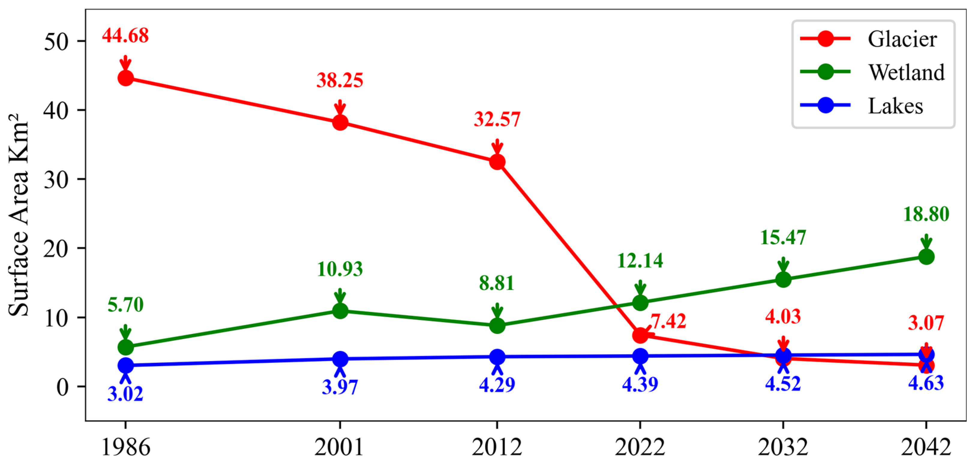
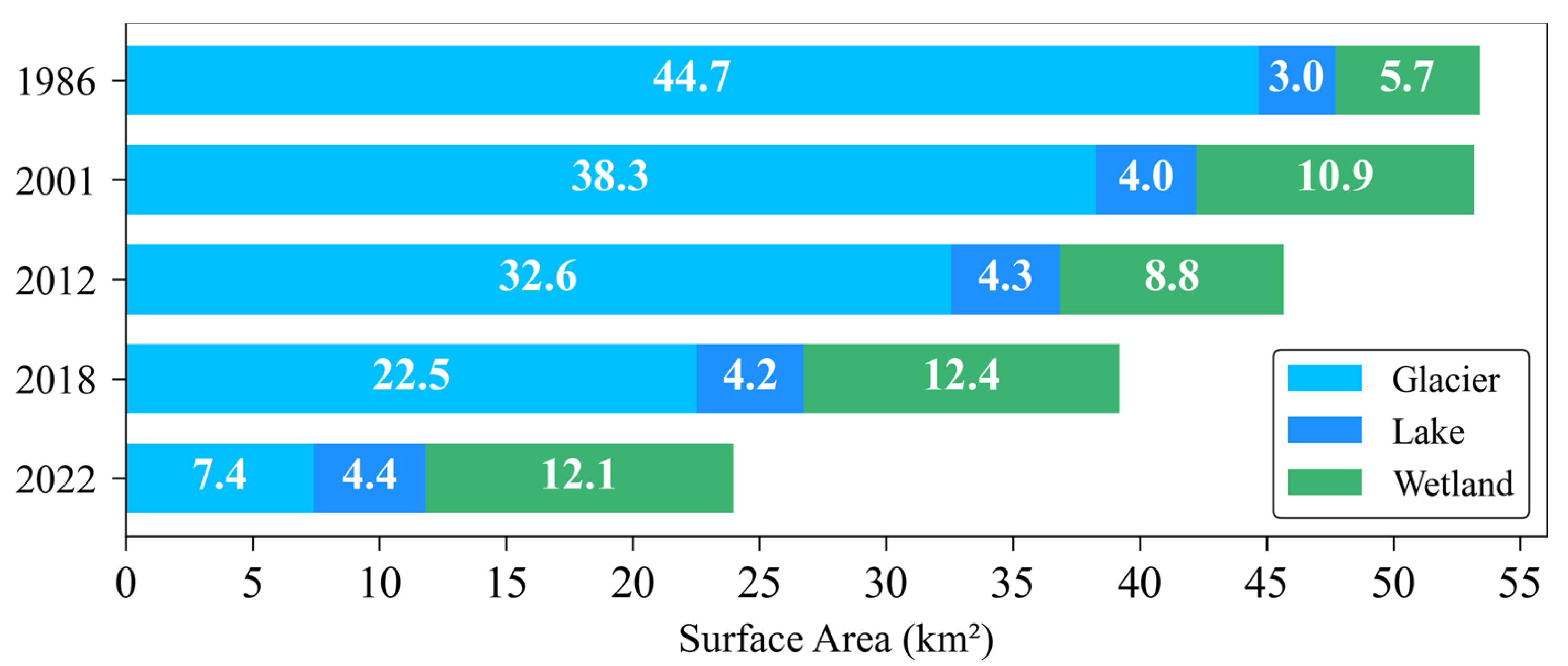
Figure 7 shows the variation in the areas in the three elements analyzed in this work. It can be observed that the lakes have not registered significant changes. In this sense, the analysis of results focuses on the glaciers and wetlands.

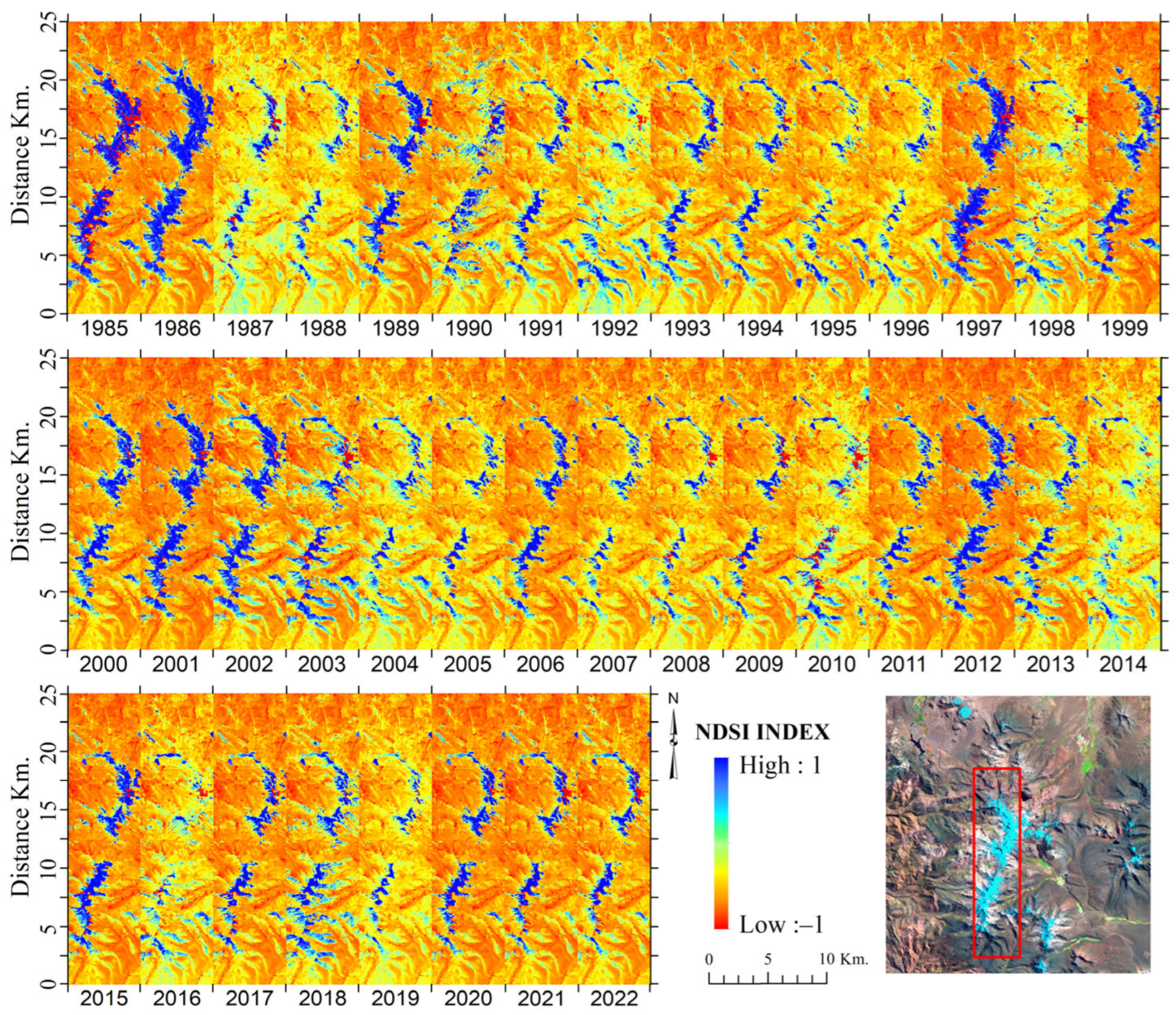
Figure 8 shows the time series of the NDSI, which reveals a prevalence of high values in the years 1985, 1986, 1989, 1997, 2000, 2001, 2002, and 2012, indicating greater snow coverage in these periods. In contrast, in the other years low values predominate, reflecting less snow coverage. The interannual variability shows that climatic factors, such as temperature and winter precipitation, exert a determining influence on the coverage and altitude of the snowline [45]. The analysis of the box plots shown in Figure 9 provides complementary evidence to the time series images, confirming the fluctuations in snow coverage, depending on the values of the NDSI. This correlation reinforces the interpretation that climatic conditions and other environmental factors may have contributed to these declines.

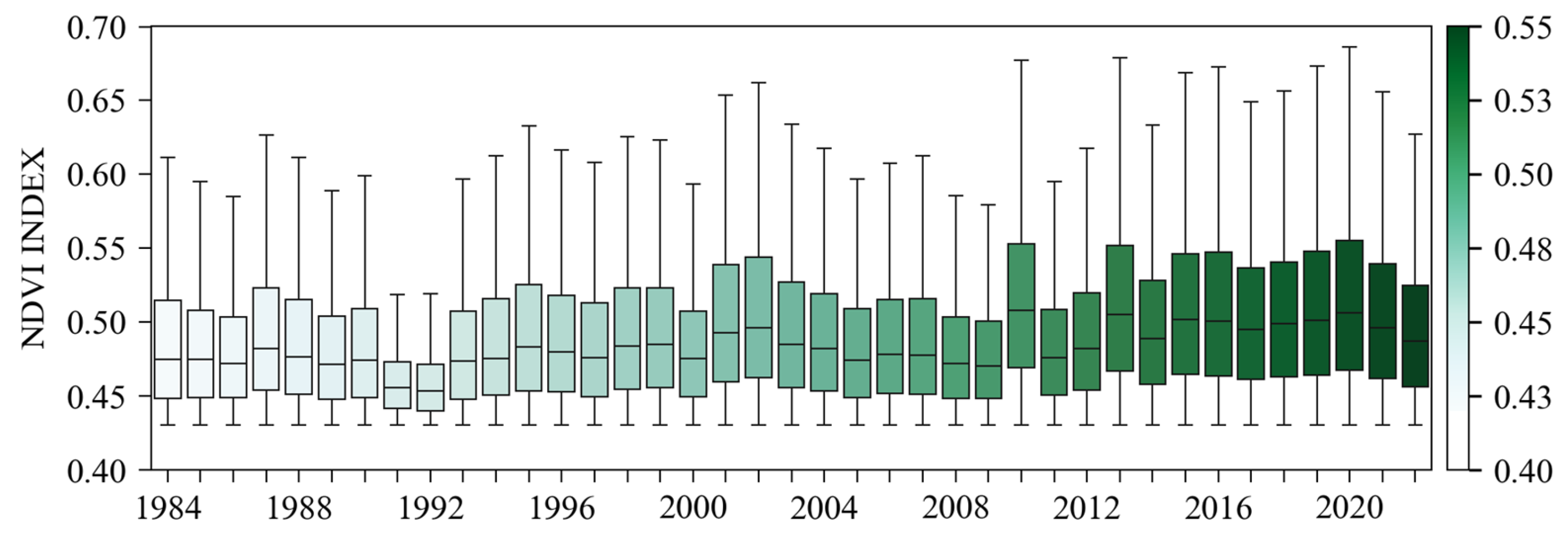
Figure 10 shows the time series of the NDVI index, the color scale ranging between −1 and 0.71. Greener colors indicate a greater density of vegetation, while purple and yellow represent less vegetation or areas without vegetation cover. Throughout the multi-year series, the patterns of vegetation loss or gain cannot be identified; in this sense, we rely on the box plots in Figure 11.

A gradual increase in the average NDVI is observed throughout the period, which could be interpreted as a general improvement in the vegetation density or in the ecological conditions of the region. In recent years, since 2000, the boxes have been taller and shifted towards higher NDVI values. Likewise, the whiskers show relatively low median values in the years 1991 and 1992, with a correlation with the NDSI, which suggests possible unfavorable conditions, such as droughts, deforestation, local fluctuations, or extreme events that affected the vegetation cover.

3.5. Scenarios, Future Projections

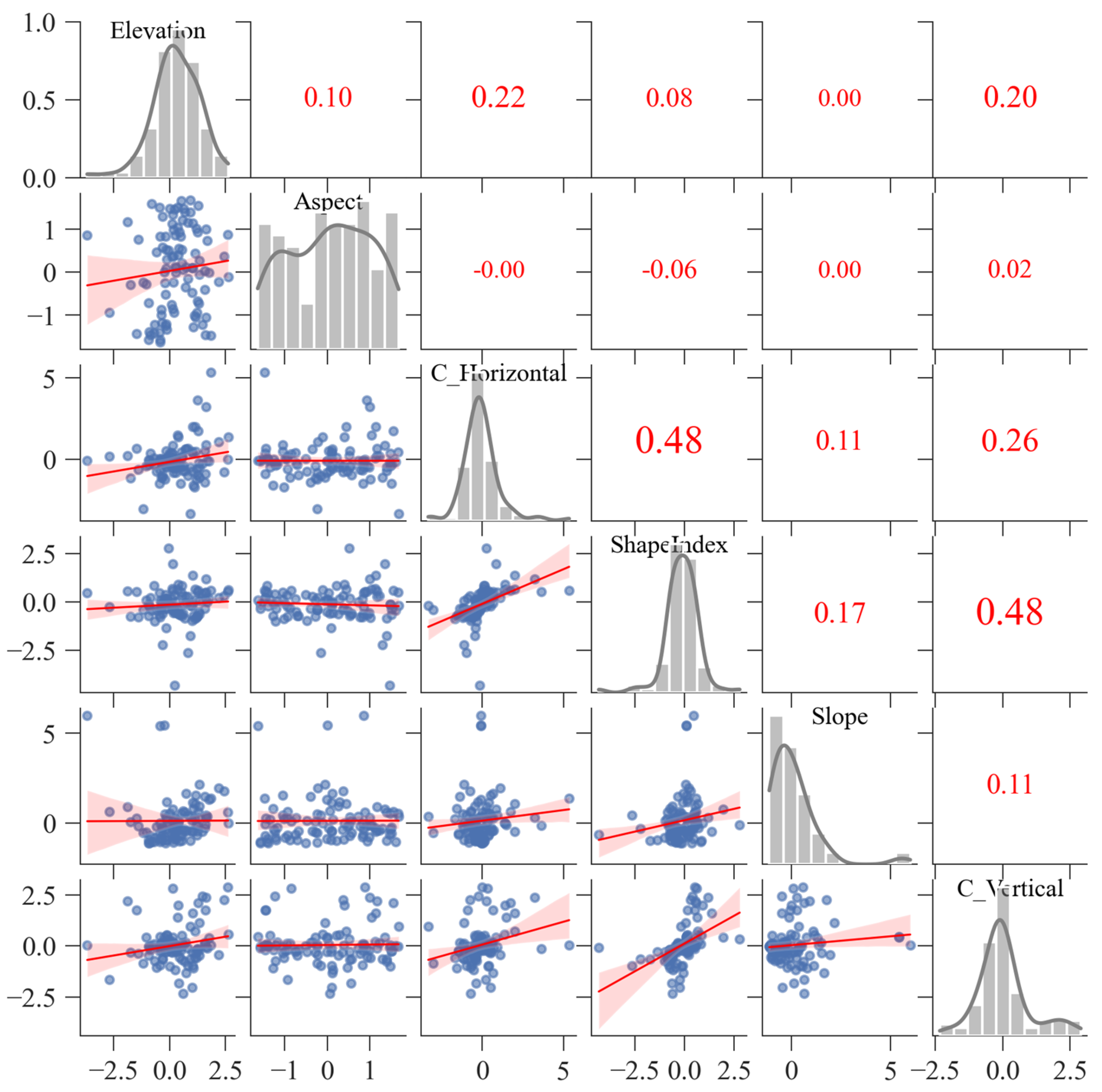
3.5.1. Evaluation of Spatial Predictor Variables

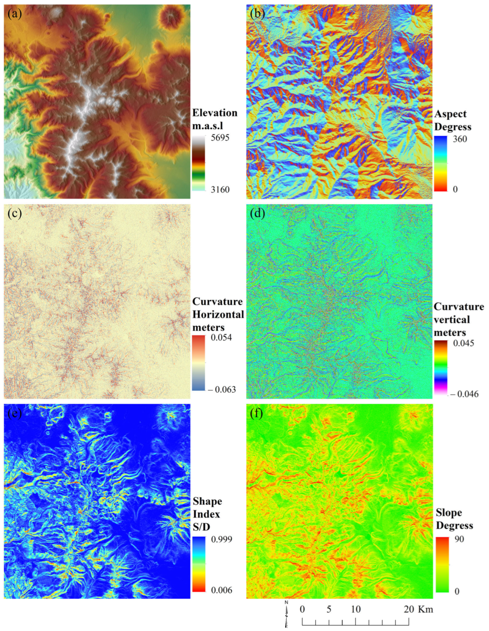
Spatial variables were processed in the MOLUSCE plugin of QGIS to analyze historical trends in land use changes and project future changes in the study area. Altitude, aspect, horizontal curvature, vertical curvature, shadow relief, and slope were included; these variables directly affect the dynamics of land use coverage [19]. Figure 12 and Figure 13 show the variables used to predict the dynamics of glaciers, lakes of glacial origin, and wetlands.

3.5.2. Modeling Transition Potential

The modeling of the transition potential in MOLUSCE-generated area changes statistics and a transition probability matrix for the study area. The results show a percentage decrease in glacier cover of 1.73% between 2012 and 2022. In contrast, there was a greater gain for the wetland class at 0.22%, as well as a slight increase in the water bodies class at 0.007%, and the other coverages class recorded an increase of 1.49%. Additionally, the transition probability matrix also revealed that the wetland and water bodies classes were the most stable and maintained their state during the 2012–2022 analysis period, reporting a change probability of 0.84 and 0.94, respectively.

3.5.3. Future Scenario Validation Model

The model was prepared for simulation using the land use maps of 2001 and 2012 to predict the land use map of 2022. The result of the prediction was the simulated map for 2022 and was validated with the classified map for the same year, reporting an accuracy of 84%. The MOLUSCE model allowed a map comparison to be carried out. For the prediction to 2032 and 2042, a total of 4000 stratified sampling points and a 3 × 3 neighborhood were used for the ANN learning process. The following inputs were used to customize the model: a learning rate of 0.001 pulse, 0.05 with 100 maximum iterations and 10 hidden layers. The overall Kappa coefficient achieved after 100 iterations in MOLUSCE was 72%, which can be considered an acceptable precision.

While the Ca–Markov model provides valuable insights into land cover transitions, its accuracy depends on assumptions about historical trends that will continue into the future. This model does not explicitly account for changing climate conditions, extreme weather events, or changes in human activity, which can influence glacier retreat and wetland stability. Integrating regional climate models (RCMs) or hydrologic models could improve the reliability of future projections by incorporating temperature and precipitation variability.

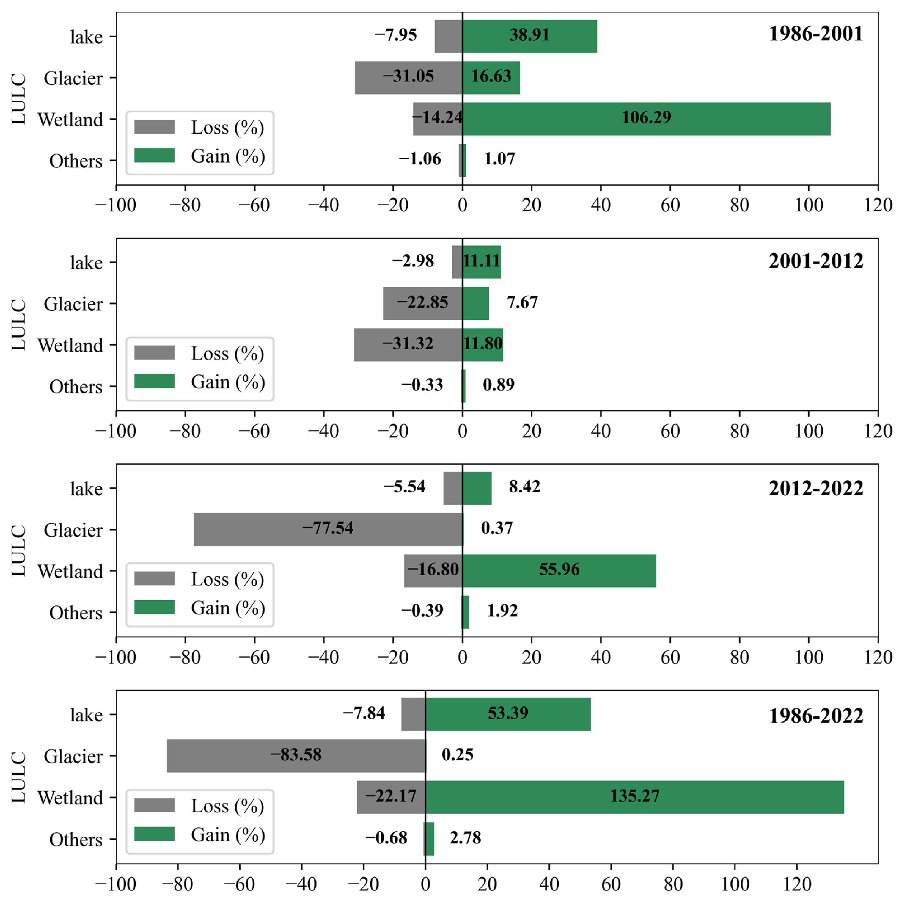
3.6. Estimation of Historical and Future Changes

The gain and loss metrics due to coverage of historical data (Figure 14) reveal that, in the period from 1986 to 2001, the surface of the wetland class maintained the greatest net change of 92.04%, followed by the bodies of water (30.96%) and glacier (14.42%), with gains of 106.29%, 38.91%, and 16.63%.

In the second period (2001–2012), the greatest net change occurred in the class of wetlands (BO) (19.52%), glaciers (GL) (15.18%), and bodies of water (CA) (8.13%) with gains of 11.80%, 11.11%, and 7.67%, respectively. In the third period (2012–2022), the GL and BO classes reported the largest net changes with 77.17 and 39.15%, and the gains were 0.37% and 55.96%. In the first period, classes GL, BO, and CA reported losses on their surfaces between 7.95 and 31.05%. This could be related to climate change and being in an arid area with accumulated annual precipitation of 400 mm [46]. In the second and third periods, the patterns are repeated in the GL classes with surface losses of up to 77.54%. In the case of CA and BO, it could be related to the dynamics of glacier coverage.

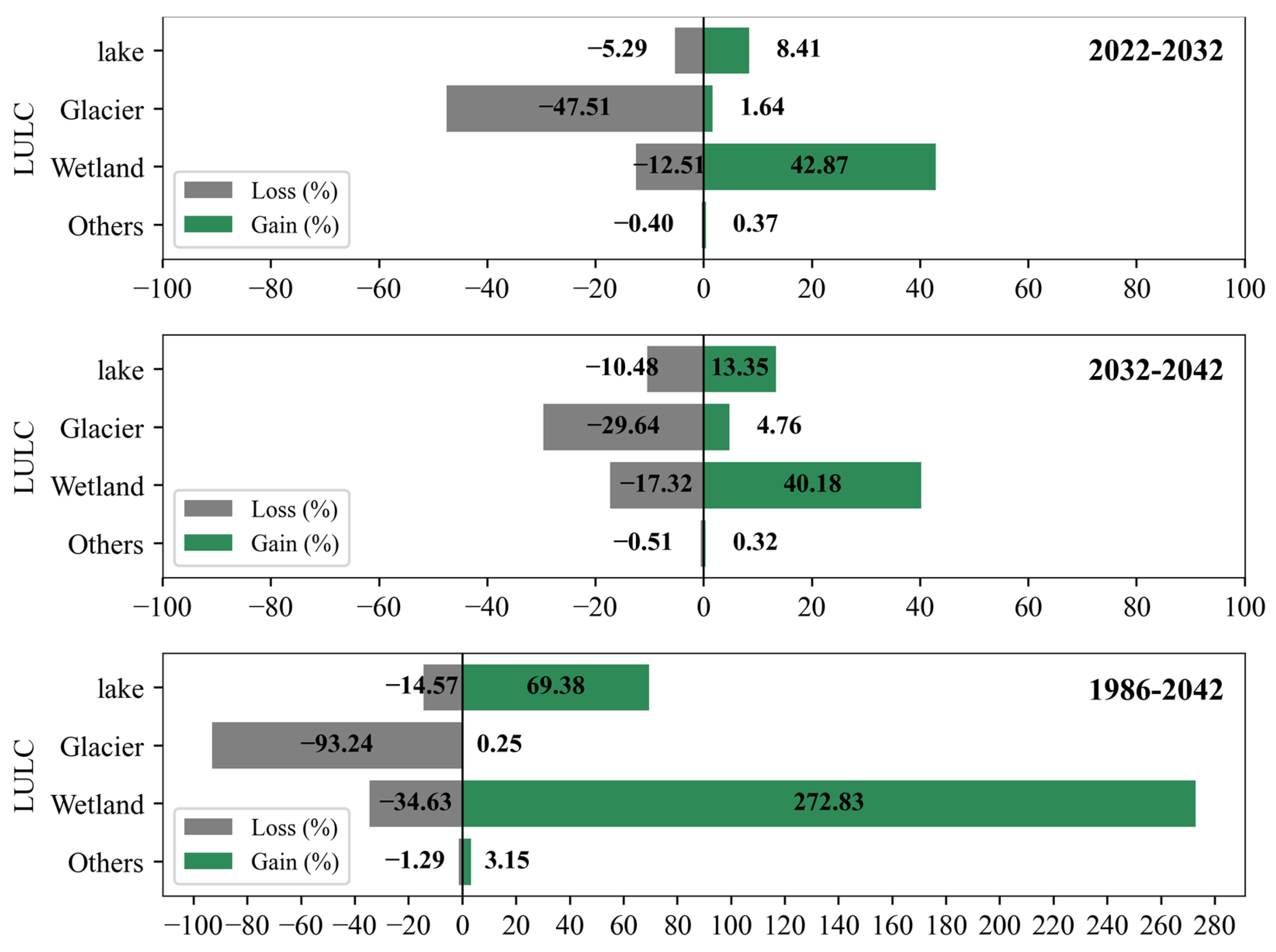
Figure 15 presents the gain and loss metrics corresponding to each land cover category, obtained from the data predicted by the model, highlighting the most significant transformation patterns throughout the study period. In the period (2022–2032) the GL class shows a significant decrease in surface area by 47.51% while the BO class experiences an increase of 42.87%. This scenario is repeated in the period 2032–2042 with the additional loss of the GL class by 29.64% and an increase of 40.18% in the BO class. Likewise, in the scenario of the observed and predicted period 1986–2042, a drastic reduction of 93.24% in the GL surface is observed, accompanied by a notable growth of 272.83% in BO and 69.38% in CA. These results provide a solid basis for evaluating the potential impacts of such changes and for designing strategies for sustainable management of natural resources.

The reduction in glacial cover (Figure 15) suggests a potential decline in meltwater contributions to the Caplina River system, which may lead to lower flows during the dry season. However, wetland expansion could provide temporary water storage, mitigating immediate losses but not compensating for long-term reductions in baseflow. Studies in other Andean basins indicate that glacier-fed rivers experience a phase shift, where peak flows shift earlier in the year due to reduced ice reserves [47].

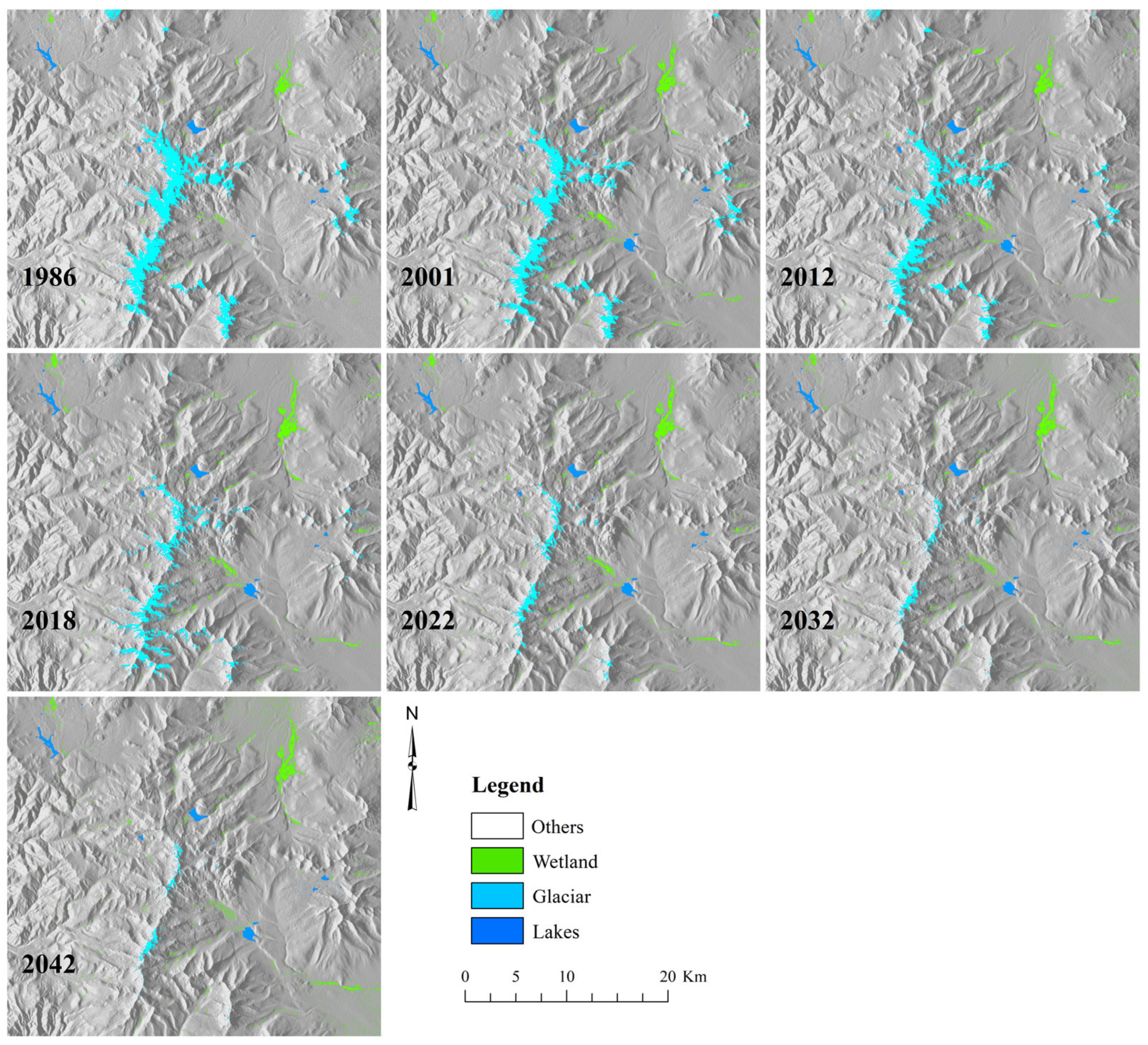
Figure 16 and Figure 17 show the historical and future distribution of the analyzed surfaces. A decrease in glacial extension and redistribution of wetlands and bodies of water is observed, which shows transformations in glacial systems due to the effects of climate change and its implications on the ecosystem services of the area. The estimate of future changes in the surface of the glaciers indicates that by 2032, it will be 4.03 km², while by 2042, it will decrease to 3.07 km², which represents a total reduction of 0.96 km². As for wetlands, a significant increase is projected: by 2032, their surface area will increase by 15.47 km² and will continue to grow until reaching a cumulative increase of 18.80 km² in 2042. On the other hand, bodies of water will show a slight increase, moving to a surface area of 4.52 km² in 2032 and reaching 4.63 km² by 2042.

These changes reflect a panorama of transformation in ecosystems due to the impact of factors such as climate change. The reduction in glaciers could have repercussions on the availability of water resources, while the growth of wetlands and bodies of water suggests modifications in humidity and water storage patterns. These data underline the need to implement sustainable management strategies to mitigate adverse effects and take advantage of changes in a beneficial way.

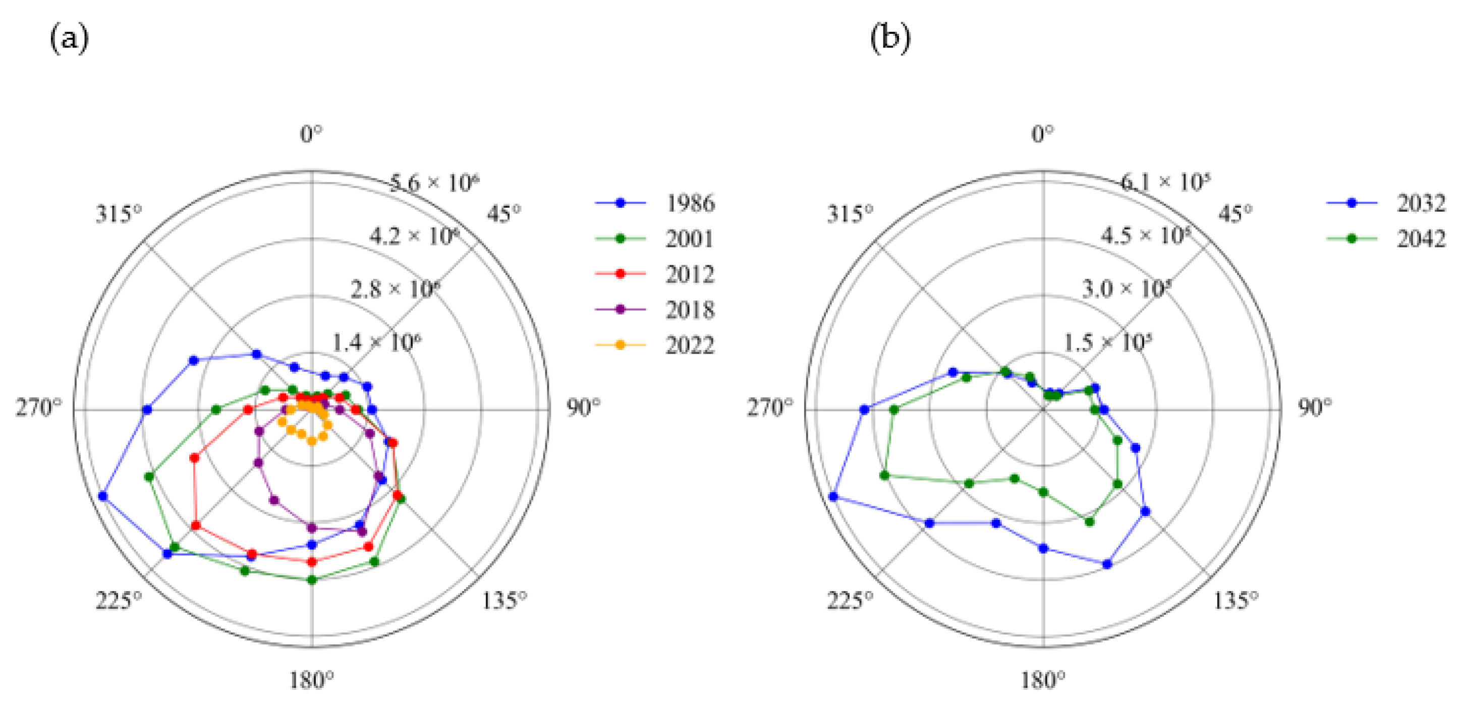
Figure 18 presents a polar diagram that shows the loss of glacial coverage due to historical and projected orientations. A marked Andean orientation stands out from northwest to southeast, corresponding to the divortium aquarum, which divides the Atlantic hydrographic unit to the northeast and the Pacific hydrographic unit to the south. In the latter are the sources of the Caplina River basin, which flows predominantly in a northeast–southwest direction until it reaches the Pacific Ocean.

In the study area, the Caplina River originates from the precipitation and melting of snow-capped mountains associated with the Barroso mountain range. According to the graph, the northeast orientation shows a decrease in glacial coverage from 2032 to 2042, which suggests a loss of glacial mass that could reduce the surface flow of the Caplina River, affecting its flow, especially in dry seasons, by reducing the contribution of the streams and tributary rivers born in the snow-capped mountains of this mountain range.

4. Discussion

The results obtained show a significant reduction in glacial coverage, accompanied by modifications in the extension of wetlands and bodies of water in the Barroso Mountain Range. These changes reflect the interaction between climate change and anthropogenic activities in the dynamics of high mountain ecosystems, highlighting the vulnerability of these environments to environmental alterations and increasing human pressure.

The analysis of the NDSI and NDVI indices shows that snow and vegetation coverage are being affected by climatic and environmental factors, which suggests a direct relationship with the variability in winter temperature and precipitation [45]. The identification of trends in both time series indicates that extreme events and long-term changes are altering the water availability and stability of high Andean ecosystems. The reduction in snow not only compromises the dynamics of wetlands and glacial lakes but could also modify the biogeochemical cycles and energy balance in the region. Given this scenario, continuous monitoring and the development of adaptation strategies are essential to mitigate impacts on water resources and biodiversity.

In this work, it was found that there is a sustained reduction in the glacier surface between 1984 and 2022. Previous studies have identified similar trends in other Andean regions, where glacial retreat has had an impact on water availability and ecosystem stability [48,49,50]. This process has increased surface water flow in the short term [51]. However, this trend may not be sustainable in the long term, given that the continued decline of glaciers would compromise the water supply in the region.

On the other hand, it is revealed that lower altitude areas have experienced the greatest impact of glacial retreat, with a considerable loss of surface below 5150 m.a.s.l. This finding is consistent with previous studies on the effects of climate change in glacial areas [52,53]. Likewise, the spatial distribution of glacial retreat suggests a more pronounced decrease in the northern and eastern orientations. This trend indicates that the melting rate is influenced by morphological and topographic factors and differential exposure to solar radiation [54,55].

In contrast, an expansion of wetlands and bodies of water has been observed, possibly related to the water supply from glacial melt. Previous research [55] has documented that the reduction in glacial cover favors the increase in water levels in wetlands and lakes, supporting the findings of the present study. However, this phenomenon could be transitory: as the glaciers continue to retreat, water flow will decrease, which could affect the sustainability of these ecosystems. The persistence of wetlands and bodies of water will depend on the availability of alternative water sources and the adaptive capacity of ecosystems in the face of these changes.

In the predictive analysis of changes in land use and cover (LULC), the hybrid CA–MARKOV model is presented as a valuable tool. However, its performance largely depends on the stability of historical LULC patterns [52]. Furthermore, its ability to generate accurate spatial predictions may be limited in scenarios of high temporal and spatial variability. Since land use changes are strongly influenced by human activity and regional planning policies, the prediction of these phenomena cannot reach absolute accuracy.

The accuracy of the Ca–Markov model bases its predictions on transition probabilities calculated from historical changes. The combination with hydrological and artificial intelligence models would allow complex environmental dynamics to be captured [56]. Furthermore, the inclusion of socio-environmental variables, such as urban expansion and land use policies, would more realistically reflect human influence on landscape changes, while the incorporation of climate scenarios and extreme events would strengthen the predictive capacity of the model.

To improve the reliability of projections, it is essential to complement these models with updated data and interdisciplinary approaches that integrate climatic, ecological and socioeconomic variables. Despite these limitations, dynamic models remain key tools in formulating hypotheses and making strategic decisions about land cover evolution. LULC projections have been widely recognized as fundamental instruments in the management of natural resources, facilitating the design of mitigation and conservation strategies to minimize environmental impacts and guarantee sustainable use of the territory [55,57,58,59].

Historically, the Caplina River has been susceptible to flash flooding, especially during periods of rain [47,60]. Precipitation and melting of the glaciers of the Barroso mountain range in the Andean zone cause an increase in the main flows of the basin [8,61,62]. The Caplina and Uchusuma rivers converge, activating the Seco River, which crosses the district of Gregorio Albarracín and flows into the Los Palos Spa in the Pacific Ocean. Evapotranspiration is fundamental in hydrological processes and plays an important role in water balances, which give rise to abrupt discharges from rivers, especially in arid areas, such as the headland of the Atacama Desert [63].

Given the evidence of the retreat of the glacial surface and its implications for water availability, it is essential to comprehensively address the impacts in downstream areas. Not only does it alter the balance of high Andean ecosystems but it also compromises the supply of water for agricultural irrigation, regional supply, and the regulation of river flow, increasing vulnerability to extreme events, such as droughts and flash floods.

In this context, it is recommended that local governments and water resources’ managers strengthen real-time hydrometeorological monitoring systems to anticipate variations in water availability. Likewise, it is essential to implement efficient water resource management policies, optimize storage and distribution infrastructure, and promote innovative technologies for water conservation. Additionally, the development of risk management plans that integrate climate change adaptation strategies and specific measures for flood mitigation in highly vulnerable regions is urged, thus guaranteeing water resilience and sustainability of ecosystems and communities dependent on the resource.

The rapid glacial retreat in the Barroso Mountain Range is directly linked to the sustained increase in temperatures in Peru, with an increase of 0.75 °C in the last century and a more marked trend in recent decades [64]. This phenomenon has altered water availability in high Andean ecosystems, generating a temporary increase in water bodies due to the greater melt flow.

5. Conclusions

This study analyzed the historical and projected land cover transformations of glaciers, wetlands, and lagoons in the Barroso mountain range, located within the hyperarid Atacama Desert. Deming linear regressions highlighted a constant retreat of glaciers and a progressive growth in wetlands and glacial lakes, supported by 95% confidence bands, allowing trends and their variability to be accurately assessed. A sixth-degree polynomial correlation complemented this analysis, capturing the complexity of temporal fluctuations and providing a more detailed representation of ecosystem transformation processes.

Using geographic information systems and cloud processing techniques in combination with cellular automata, we evaluated glacier retreat and its influence on land cover and land use changes. The analysis identified three land cover types: glaciers, wetlands, and bodies of water. Over the last 36 years, glaciers experienced a drastic decline from 44.7 km² to 7.4 km², while bodies of water and wetlands expanded by 1.4 km² and 6.4 km², respectively. These dynamics reflect a substantial transformation of high mountain ecosystems, probably influenced by glacial retreat and changes in precipitation patterns.

The accelerated retreat of glaciers in the Barroso range is consistent with broader global trends of cryospheric change. Similar patterns have been documented in the Cordillera Blanca, Peru, and the Bolivian Andes, where glacier loss is significantly altering regional hydrological balances. These findings contribute to the growing body of research on glacier-fed water systems in arid and semi-arid environments and highlight the urgent need for sustainable water management strategies in the face of increasing climate variability. The analysis of the glacier distribution coverage based on elevations reveals very clear patterns; in 1986, most glacier coverage was between 4950 m.a.s.l. and 7750 m.a.s.l. Since 2001, the reduction was most notable at lower elevations, with a total disappearance below 4950 m.a.s.l. in 2012. By 2022, the lowest elevations reached 5150 m.a.s.l., reflecting a loss of approximately 200 m. This pattern highlights the greater vulnerability of glacial areas at lower altitudes, highlighting the impact of climate change in these areas.

Orientation analysis of glacier loss indicates a decrease in 1986, the south and west orientations concentrated most of the glacier mass. Beginning in 2001, the loss was most pronounced in north and east orientations, with a complete disappearance of coverage in those directions. By 2018, the glaciers disappeared from the west orientation, and in 2022, only remnants remained on the south orientation. This pattern reflects the accelerated reduction in glaciers.

The time series analysis of NDSI and NDVI indices shows fluctuations in snow and vegetation coverage over time. Snow peaks occurred in 1985, 1986, 1989, 1997, 2000, 2001, 2002, and 2012, while periods of lower coverage were recorded in 1992, 1998, 2016, and 2024. Since 2000, the NDVI index has shown an increase in vegetation density, although low values in 1991 and 1992 suggest adverse climatic events that affected both snow and vegetation.

Analysis of observed coverage gains and losses between 1986 and 2022 shows that wetlands (BO) experienced the largest increase, especially between 1986 and 2001, with an increase of 92.04%. Glaciers (GL) and bodies of water (CA) also increased but to a lesser extent. Between 2001 and 2012, glaciers began to reduce their surface, while the wetlands continued to grow. From 2012 to 2022, glaciers lost 77.17% of their area, while wetlands increased by 39.15%. These changes are linked to climate change and the arid conditions of the region.

The modeling of future scenarios carried out from the land cover and use maps and MOLUSCE showed that projections for the next few years indicate a drastic reduction in glacier cover (GL), with an estimated loss of 93.24% between 1986 and 2042. This decrease is accompanied by a notable growth of wetlands (BO), which could increase by 272.83% in the same period. In addition, bodies of water (CA) will also experience growth, although to a lesser extent of 69.38%.

The Caplina River demonstrates a transformative dynamic influenced by climatic factors, such as exceptional rainfall in the Andean zone. These rains cause an increase in the flow in the basin, activating dry channels and generating a risk of flash floods in urbanized areas along their route. This phenomenon, similar to the glacial retreat observed in other regions, reflects an alteration of natural patterns and a greater vulnerability of the low areas of the Caplina basin, especially the Seco River ravine, which runs alongside the city of Tacna, which highlights the need for greater attention to the effects of climate change on the basins and surrounding ecosystems.

While the observed expansion of wetlands suggests a temporary increase in available water from glacial melt, the long-term sustainability of these ecosystems remains uncertain. As glaciers continue to retreat, meltwater contributions are likely to decrease, potentially leading to a change in wetland hydrodynamics and a decrease in water storage capacity. This could impact downstream hydrology, particularly in semiarid basins such as the Quebrada del Río Seco. Future studies should investigate the resilience of these wetlands under scenarios of prolonged glacial loss.

The results of this study underscore the urgency of implementing adaptive water management strategies in glacier-dependent watersheds. Given the projected decline in glacier mass and potential changes in wetland dynamics, policymakers should prioritize integrated water resources planning considering both short-term hydrological changes and long-term sustainability challenges. Future efforts should focus on developing mitigation strategies that balance ecosystem conservation with human water needs in a rapidly changing climate.

References

- Gómez-Silva, B.; Batista-García, R.A. The Atacama Desert: A Biodiversity Hotspot and Not Just a Mineral-Rich Region. Front. Microbiol. 2022, 13, 812842. [Google Scholar] [CrossRef] [PubMed]
- Ritter, B.; Wennrich, V.; Medialdea, A.; Brill, D.; King, G.; Schneiderwind, S.; Niemann, K.; Fernández-Galego, E.; Diederich, J.; Rolf, C.; et al. Climatic Fluctuations in the Hyperarid Core of the Atacama Desert during the Past 215 Ka. Sci. Rep. 2019, 9, 5270. [Google Scholar] [CrossRef] [PubMed]
- Eshel, G.; Araus, V.; Undurraga, S.; Soto, D.C.; Moraga, C.; Montecinos, A.; Moyano, T.; Maldonado, J.; Díaz, F.P.; Varala, K.; et al. Plant Ecological Genomics at the Limits of Life in the Atacama Desert. Proc. Natl. Acad. Sci. USA 2021, 118, e2101177118. [Google Scholar] [CrossRef] [PubMed]
- Pino-Vargas, E. Caplina Aquifer, after 100 Years of Exploitation as a Sustenance for Agriculture in Arid Zones. Proc. IAHR World Congr. 2022, 2928, 090004. [Google Scholar]
- Pino-Vargas, E.; Espinoza-Molina, J.; Chávarri-Velarde, E.; Quille-Mamani, J.; Ingol-Blanco, E. Impacts of Groundwater Management Policies in the Caplina Aquifer, Atacama Desert. Water 2023, 15, 2610. [Google Scholar] [CrossRef]
- Pino-Vargas, E.; Ascencios-Templo, D. La Implementación de Veda Como Una Herramienta Para Controlar La degradación del Acuífero Costero La Yarada, Tacna, Perú. Diálogo Andin. 2021, 66, 489–496. [Google Scholar] [CrossRef]
- Pocco, V.; Chucuya, S.; Huayna, G.; Ingol-Blanco, E.; Pino-Vargas, E. A Multi-Criteria Decision-Making Technique Using Remote Sensors to Evaluate the Potential of Groundwater in the Arid Zone Basin of the Atacama Desert. Water 2023, 15, 1344. [Google Scholar] [CrossRef]
- González-Domínguez, J.; Mora, A.; Chucuya, S.; Pino-Vargas, E.; Torres-Martínez, J.A.; Dueñas-Moreno, J.; Ramos-Fernández, L.; Kumar, M.; Mahlknecht, J. Hydraulic Recharge and Element Dynamics during Salinization in an Overexploited Coastal Aquifer of the World’s Driest Zone: Atacama Desert. Sci. Total Environ. 2024, 954, 176204. [Google Scholar] [CrossRef]
- Zhang, Z.; Hu, B.; Jiang, W.; Qiu, H. Identification and Scenario Prediction of Degree of Wetland Damage in Guangxi Based on the CA-Markov Model. Ecol. Indic. 2021, 127, 107764. [Google Scholar] [CrossRef]
- Pfeiffer, M.; Latorre, C.; Santoro, C.M.; Gayo, E.M.; Rojas, R.; Carrevedo, M.L.; McRostie, V.B.; Finstad, K.M.; Heimsath, A.; Jungers, M.C.; et al. Chronology, Stratigraphy and Hydrological Modelling of Extensive Wetlands and Paleolakes in the Hyperarid Core of the Atacama Desert during the Late Quaternary. Quat. Sci. Rev. 2018, 197, 224–245. [Google Scholar] [CrossRef]
- Finstad, K.; Pfeiffer, M.; McNicol, G.; Barnes, J.; Demergasso, C.; Chong, G.; Amundson, R. Rates and Geochemical Processes of Soil and Salt Crust Formation in Salars of the Atacama Desert, Chile. Geoderma 2016, 284, 57–72. [Google Scholar] [CrossRef]
- Surabuddin Mondal, M.; Sharma, N.; Kappas, M.; Garg, P.K. Modeling of Spatio-Temporal Dynamics of Land Use and Land Cover in a Part of Brahmaputra River Basin Using Geoinformatic Techniques. Geocarto Int. 2013, 28, 632–656. [Google Scholar] [CrossRef]
- Yulianto, F.; Maulana, T.; Khomarudin, M.R. Analysis of the Dynamics of Land Use Change and Its Prediction Based on the Integration of Remotely Sensed Data and CA-Markov Model, in the Upstream Citarum Watershed, West Java, Indonesia. Int. J. Digit. Earth 2019, 12, 1151–1176. [Google Scholar] [CrossRef]
- Liu, C.; Song, W.; Lu, C.; Xia, J. Spatial-Temporal Hidden Markov Model for Land Cover Classification Using Multitemporal Satellite Images. IEEE Access 2021, 9, 76493–76502. [Google Scholar] [CrossRef]
- Zhu, Z. Change Detection Using Landsat Time Series: A Review of Frequencies, Preprocessing, Algorithms, and Applications. ISPRS J. Photogramm. Remote Sens. 2017, 130, 370–384. [Google Scholar] [CrossRef]
- Kozhikkodan Veettil, B.; Pereira, S.F.R.; Wang, S.; Valente, P.T.; Grondona, A.E.B.; Rondón, A.C.B.; Rekowsky, I.C.; De Souza, S.F.; Bianchini, N.; Bremer, U.F.; et al. Un Análisis Comparativo Del Comportamiento Diferencial de Los Glaciares En Los Andes Tropicales Usando Teledetección. Investig. Geográficas 2016, 51, 3–36. [Google Scholar] [CrossRef]
- Veettil, B.K. Glacier Mapping in the Cordillera Blanca, Peru, Tropical Andes, Using Sentinel-2 and Landsat Data. Singap. J. Trop. Geogr. 2018, 39, 351–363. [Google Scholar] [CrossRef]
- Gorelick, N.; Hancher, M.; Dixon, M.; Ilyushchenko, S.; Thau, D.; Moore, R. Google Earth Engine: Planetary-Scale Geospatial Analysis for Everyone. Remote Sens. Environ. 2017, 202, 18–27. [Google Scholar] [CrossRef]
- Turpo-Cayo, E.Y.; Borja, M.O.; Espinoza-Villar, R.; Moreno, N.; Camargo, R.; Almeida, C.; Hopfgartner, K.; Yarleque, C.; Souza, C.M. Mapping Three Decades of Changes in the Tropical Andean Glaciers Using Landsat Data Processed in the Earth Engine. Remote Sens. 2022, 14, 1974. [Google Scholar] [CrossRef]
- Wulder, M.A.; White, J.C.; Loveland, T.R.; Woodcock, C.E.; Belward, A.S.; Cohen, W.B.; Fosnight, E.A.; Shaw, J.; Masek, J.G.; Roy, D.P. The Global Landsat Archive: Status, Consolidation, and Direction. Remote Sens. Environ. 2016, 185, 271–283. [Google Scholar] [CrossRef]
- Teixeira Pinto, C.; Jing, X.; Leigh, L. Evaluation Analysis of Landsat Level-1 and Level-2 Data Products Using In Situ Measurements. Remote Sens. 2020, 12, 2597. [Google Scholar] [CrossRef]
- Townshend, J.R.; Masek, J.G.; Huang, C.; Vermote, E.F.; Gao, F.; Channan, S.; Sexton, J.O.; Feng, M.; Narasimhan, R.; Kim, D.; et al. Global Characterization and Monitoring of Forest Cover Using Landsat Data: Opportunities and Challenges. Int. J. Digit. Earth 2012, 5, 373–397. [Google Scholar] [CrossRef]
- Amani, M.; Ghorbanian, A.; Ahmadi, S.A.; Kakooei, M.; Moghimi, A.; Mirmazloumi, S.M.; Moghaddam, S.H.A.; Mahdavi, S.; Ghahremanloo, M.; Parsian, S.; et al. Google Earth Engine Cloud Computing Platform for Remote Sensing Big Data Applications: A Comprehensive Review. IEEE J. Sel. Top. Appl. Earth Obs. Remote Sens. 2020, 13, 5326–5350. [Google Scholar] [CrossRef]
- Markert, K. Cartoee: Publication Quality Maps Using Earth Engine. J. Open Source Softw. 2019, 4, 1207. [Google Scholar] [CrossRef]
- Herreid, S.; Pellicciotti, F. The State of Rock Debris Covering Earth’s Glaciers. Nat. Geosci. 2020, 13, 621–627. [Google Scholar] [CrossRef]
- Salomonson, V.V.; Appel, I. Estimating Fractional Snow Cover from MODIS Using the Normalized Difference Snow Index. Remote Sens. Environ. 2004, 89, 351–360. [Google Scholar] [CrossRef]
- Qiao, C.; Luo, J.; Sheng, Y.; Shen, Z.; Zhu, Z.; Ming, D. An Adaptive Water Extraction Method from Remote Sensing Image Based on NDWI. J. Indian Soc. Remote Sens. 2012, 40, 421–433. [Google Scholar] [CrossRef]
- Gao, B. NDWI—A Normalized Difference Water Index for Remote Sensing of Vegetation Liquid Water from Space. Remote Sens. Environ. 1996, 58, 257–266. [Google Scholar] [CrossRef]
- Corripio, J.G. Vectorial Algebra Algorithms for Calculating Terrain Parameters from DEMs and Solar Radiation Modelling in Mountainous Terrain. Int. J. Geogr. Inf. Sci. 2003, 17, 1–23. [Google Scholar] [CrossRef]
- Farr, T.G.; Rosen, P.A.; Caro, E.; Crippen, R.; Duren, R.; Hensley, S.; Kobrick, M.; Paller, M.; Rodriguez, E.; Roth, L.; et al. The Shuttle Radar Topography Mission. Rev. Geophys. 2007, 45. [Google Scholar] [CrossRef]
- Macander, M.J.; Swingley, C.S.; Joly, K.; Raynolds, M.K. Landsat-Based Snow Persistence Map for Northwest Alaska. Remote Sens. Environ. 2015, 163, 23–31. [Google Scholar] [CrossRef]
- Hanshaw, M.N.; Bookhagen, B. Glacial Areas, Lake Areas, and Snow Lines from 1975 to 2012: Status of the Cordillera Vilcanota, Including the Quelccaya Ice Cap, Northern Central Andes, Peru. Cryosphere 2014, 8, 359–376. [Google Scholar] [CrossRef]
- White, D.C.; Lewis, M.M.; Green, G.; Gotch, T.B. A Generalizable NDVI-Based Wetland Delineation Indicator for Remote Monitoring of Groundwater Flows in the Australian Great Artesian Basin. Ecol. Indic. 2016, 60, 1309–1320. [Google Scholar] [CrossRef]
- Kaplan, G.; Avdan, U. Mapping and Monitoring Wetlands Using Sentinel-2 Satellite Imagery. ISPRS Ann. Photogramm. Remote Sens. Spat. Inf. Sci. 2017, IV-4/W4, 271–277. [Google Scholar] [CrossRef]
- Ashok, A.; Rani, H.P.; Jayakumar, K.V. Monitoring of Dynamic Wetland Changes Using NDVI and NDWI Based Landsat Imagery. Remote Sens. Appl. Soc. Environ. 2021, 23, 100547. [Google Scholar] [CrossRef]
- Xu, C.; Qu, J.J.; Hao, X.; Wu, D. Monitoring Surface Soil Moisture Content over the Vegetated Area by Integrating Optical and SAR Satellite Observations in the Permafrost Region of Tibetan Plateau. Remote Sens. 2020, 12, 183. [Google Scholar] [CrossRef]
- Sriwongsitanon, N.; Gao, H.; Savenije, H.H.G.; Maekan, E.; Saengsawang, S.; Thianpopirug, S. Comparing the Normalized Difference Infrared Index (NDII) with Root Zone Storage in a Lumped Conceptual Model. Hydrol. Earth Syst. Sci. 2016, 20, 3361–3377. [Google Scholar] [CrossRef]
- Hunt, J.E.R.; Yilmaz, M.T. Remote Sensing of Vegetation Water Content Using Shortwave Infrared Reflectances; Gao, W., Ustin, S.L., Eds.; 2007; p. 667902. Available online: https://www.spiedigitallibrary.org/conference-proceedings-of-spie/6679/1/Remote-sensing-of-vegetation-water-content-using-shortwave-infrared-reflectances (accessed on 28 February 2025). [CrossRef]
- Torres, M.; Pierantozzi, P.; Searles, P.; Rousseaux, M.C.; García-Inza, G.; Miserere, A.; Bodoira, R.; Contreras, C.; Maestri, D. Olive Cultivation in the Southern Hemisphere: Flowering, Water Requirements and Oil Quality Responses to New Crop Environments. Front. Plant Sci. 2017, 8, 1830. [Google Scholar] [CrossRef]
- Ni, W.; Yu, T.; Pang, Y.; Zhang, Z.; He, Y.; Li, Z.; Sun, G. Seasonal Effects on Aboveground Biomass Estimation in Mountainous Deciduous Forests Using ZY-3 Stereoscopic Imagery. Remote Sens. Environ. 2023, 289, 113520. [Google Scholar] [CrossRef]
- Garcia, D.J.; Willems, B.; Espinoza, V.R. Mapeo de Bofedales En Cabeceras de Cuenca Mediante Imágenes de Los Satélites Landsat. Rev. Glaciares y Ecosistemas Montaña 2016, 38, 92–108. [Google Scholar]
- Polk, M.H.; Young, K.R.; Baraer, M.; Mark, B.G.; McKenzie, J.M.; Bury, J.; Carey, M. Exploring Hydrologic Connections between Tropical Mountain Wetlands and Glacier Recession in Peru’s Cordillera Blanca. Appl. Geogr. 2017, 78, 94–103. [Google Scholar] [CrossRef]
- Knipling, E.B. Physical and Physiological Basis for the Reflectance of Visible and Near-Infrared Radiation from Vegetation. Remote Sens. Environ. 1970, 1, 155–159. [Google Scholar] [CrossRef]
- Mas, J.-F.; Kolb, M.; Paegelow, M.; Camacho Olmedo, M.T.; Houet, T. Inductive Pattern-Based Land Use/Cover Change Models: A Comparison of Four Software Packages. Environ. Model. Softw. 2014, 51, 94–111. [Google Scholar] [CrossRef]
- Aranda, F.; Medina, D.; Castro, L.; Ossandón, Á.; Ovalle, R.; Flores, R.P.; Bolaño-Ortiz, T.R. Snow Persistence and Snow Line Elevation Trends in a Snowmelt-Driven Basin in the Central Andes and Their Correlations with Hydroclimatic Variables. Remote Sens. 2023, 15, 5556. [Google Scholar] [CrossRef]
- Rau, P.; Bourrel, L.; Labat, D.; Ruelland, D.; Frappart, F.; Lavado, W.; Dewitte, B.; Felipe, O. Assessing Multidecadal Runoff (1970–2010) Using Regional Hydrological Modelling under Data and Water Scarcity Conditions in Peruvian Pacific Catchments. Hydrol. Process. 2019, 33, 20–35. [Google Scholar] [CrossRef]
- Pino-Vargas, E.; Eduardo, C.V. Evidence of Climate Change in the Hyper-Arid Region of the Southern Coast of Peru, Head of the Atacama Desert. Tecnol. y Ciencias del Agua 2022, 13, 333–376. [Google Scholar] [CrossRef]
- Cepeda Arias, E.; Cañon Barriga, J.; Salazar, J.F. Changes of Streamflow Regulation in an Andean Watershed with Shrinking Glaciers: Implications for Water Security. Hydrol. Sci. J. 2022, 67, 1755–1770. [Google Scholar] [CrossRef]
- Caro, A.; Condom, T.; Rabatel, A.; Champollion, N.; García, N.; Saavedra, F. Hydrological Response of Andean Catchments to Recent Glacier Mass Loss. Cryosphere 2024, 18, 2487–2507. [Google Scholar] [CrossRef]
- Madrigal-Martínez, S.; Puga-Calderón, R.J.; Bustínza Urviola, V.; Vilca Gómez, Ó. Spatiotemporal Changes in Land Use and Ecosystem Service Values Under the Influence of Glacier Retreat in a High-Andean Environment. Front. Environ. Sci. 2022, 10, 941887. [Google Scholar] [CrossRef]
- Vuille, M.; Francou, B.; Wagnon, P.; Juen, I.; Kaser, G.; Mark, B.G.; Bradley, R.S. Climate Change and Tropical Andean Glaciers: Past, Present and Future. Earth-Science Rev. 2008, 89, 79–96. [Google Scholar] [CrossRef]
- Thompson, L.G.; Davis, M.E.; Mosley-Thompson, E.; Porter, S.E.; Corrales, G.V.; Shuman, C.A.; Tucker, C.J. The Impacts of Warming on Rapidly Retreating High-Altitude, Low-Latitude Glaciers and Ice Core-Derived Climate Records. Glob. Planet. Chang. 2021, 203, 103538. [Google Scholar] [CrossRef]
- Cao, B.; Pan, B.; Guan, W.; Wen, Z.; Wang, J. Changes in Glacier Volume on Mt. Gongga, Southeastern Tibetan Plateau, Based on the Analysis of Multi-Temporal DEMs from 1966 to 2015. J. Glaciol. 2019, 65, 366–375. [Google Scholar] [CrossRef]
- Olson, M.; Rupper, S. Impacts of Topographic Shading on Direct Solar Radiation for Valley Glaciers in Complex Topography. Cryosphere 2019, 13, 29–40. [Google Scholar] [CrossRef]
- Asif, M.; Kazmi, J.H.; Tariq, A.; Zhao, N.; Guluzade, R.; Soufan, W.; Almutairi, K.F.; Sabagh, A.E.; Aslam, M. Modelling of Land Use and Land Cover Changes and Prediction Using CA-Markov and Random Forest. Geocarto Int. 2023, 38, 2210532. [Google Scholar] [CrossRef]
- Peng, H.; Yang, W.; Nadine Ferrer, A.S.; Xiong, S.; Li, X.; Niu, G.; Lu, T. Hydrochemical Characteristics and Health Risk Assessment of Groundwater in Karst Areas of Southwest China: A Case Study of Bama, Guangxi. J. Clean. Prod. 2022, 341, 130872. [Google Scholar] [CrossRef]
- Arfasa, G.F.; Owusu-Sekyere, E.; Doke, D.A. Predictions of Land Use/Land Cover Change, Drivers, and Their Implications on Water Availability for Irrigation in the Vea Catchment, Ghana. Geocarto Int. 2023, 38, 2243093. [Google Scholar] [CrossRef]
- Ruben, G.B.; Zhang, K.; Dong, Z.; Xia, J. Analysis and Projection of Land-Use/Land-Cover Dynamics through Scenario-Based Simulations Using the CA-Markov Model: A Case Study in Guanting Reservoir Basin, China. Sustainability 2020, 12, 3747. [Google Scholar] [CrossRef]
- Matlhodi, B.; Kenabatho, P.K.; Parida, B.P.; Maphanyane, J.G. Analysis of the Future Land Use Land Cover Changes in the Gaborone Dam Catchment Using CA-Markov Model: Implications on Water Resources. Remote Sens. 2021, 13, 2427. [Google Scholar] [CrossRef]
- Pino-Vargas, E.; Chávarri-Velarde, E.; Ingol-Blanco, E.; Mejía, F.; Cruz, A.; Vera, A. Impacts of Climate Change and Variability on Precipitation and Maximum Flows in Devil’s Creek, Tacna, Peru. Hydrology 2022, 9, 10. [Google Scholar] [CrossRef]
- Avendaño-Jihuallanga, C.; Pino-Vargas, E.; Espinoza-Molina, J.; Cabrera-Olivera, F.; Ramos-Fernández, L.; Chávarri-Velarde, E.; Ingol-Blanco, E.; Vera-Barrios, B.; Ascencios, D. El Impacto de Las Inundaciones en la Zona Norte del Desierto de Atacama: Una Revisión Histórica Sistemática de los Eventos en el Periodo 1911 A 2022. Diálogo Andin. 2024, 75, 48–67. [Google Scholar] [CrossRef]
- Machaca-Pillaca, R.; Pino-Vargas, E.; Ramos-Fernández, L.; Quille-Mamani, J.A.; Torres-Rua, A.F. Estimation of Evapotranspiration for Irrigation Purposes in Real Time of an Olive Grove from Drone Images in Arid Areas, Case of La Yarada, Tacna, Peru. Idesia 2022, 40. [Google Scholar] [CrossRef]
- Cruz-Baltuano, A.; Huarahuara-Toma, R.; Silva-Borda, A.; Chucuya, S.; Franco-León, P.; Huayna, G.; Ramos-Fernández, L.; Pino-Vargas, E. Assessment of Observed and Projected Extreme Droughts in Perú—Case Study: Candarave, Tacna. Atmosphere 2025, 16, 18. [Google Scholar] [CrossRef]
- López-Moreno, J.I.; Morán-Tejeda, E.; Vicente-Serrano, S.M.; Bazo, J.; Azorin-Molina, C.; Revuelto, J.; Sánchez-Lorenzo, A.; Navarro-Serrano, F.; Aguilar, E.; Chura, O. Recent Temperature Variability and Change in the Altiplano of Bolivia and Peru. Int. J. Climatol. 2016, 36, 1773–1796. [Google Scholar] [CrossRef]
Figure 1.
Climatic variables in the study region.
Figure 2.
Location of the study area. (a) Barroso mountain in the Andes mountain range. (b) Scheme of the glacier zone to the arid region, Seco River area, City of Tacna.
Figure 3.
Flowchart of the methodology used, modified from Turpo–Cayo (2022) [
19].
Figure 4.
Regression analysis in the cover classes. (a) Regression of glacier cover, (b) regression of lake cover, and (c) regression of wetland cover of the study area.
Figure 5.
Temporal evolution of coverage. Polynomial equations of the sixth degree provide a better representation of the complex and non-linear trends observed. Glacier: −7.7 × 10−9 x6 + 6.2 × 10−5 x5 – 0.16 x4 + 0.25 x3 + 6.2 × 105 x2 − 109 x + 5 × 10¹¹, Lakes: −9.8 × 10−11 x6 + 7.9 × 10−7 x5 – 0.002 x4 + 0.014 x3 + 8 × 103 x2 – 1.3 × 10⁷ x + 6.5 × 10⁹, Wetlands: −1.3 × 10−9 x6 + 1.1 × 10−5 x5 – 0.027 x4 – 0.016 x3 + 1.1 × 105 x2 – 1.7 × 10⁸ x + 8.5 × 10¹⁰.
Figure 6.
Spectral signature extracted from the 100 random points of (a) glacier, (b) wetlands and (c) lake. The lines of different colors represent the mean values for each class.
Figure 7.
Temporal variation and future projection of the surfaces of the analyzed elements during the period from 1986 to 2042.
Figure 8.
NDSI multi-year time series between 1985 and 2022 in the Barroso mountain range.
Figure 9.
Box plot, multi-year statistics of the NDSI glacier cover index.
Figure 10.
NDVI multi-year time series between the years 1985 to 2022, in the Barroso mountain range.
Figure 11.
Boxplot, multi-year statistics of the NDVI vegetation cover index.
Figure 12.
Correlation of predictor variables. Blue dots: Represent the individual data in each pair of variables. Each point is an observation with its values in the two corresponding variables. Red line: This is a linear regression line fitted to the data in each scatter plot. It shows the trend of the relationship between the two variables in comparison. Shaded area around the red line: Represents the confidence interval of the regression. Indicates the uncertainty in the estimate of the trend line; the wider this region, the greater the variability in the relationship between the two variables.
Figure 13.
Prediction spatial component input variables. (a) Altitude. (b) Appearance. (c) Horizontal Curvature. (d) Vertical curvature. (e) Highlight shadow. (f) Slope.
Figure 14.
Historical LULC gains and losses.
Figure 15.
Projected future profits and losses of LULCs.
Figure 16.
Historical and future distribution of surfaces lakes, glaciers, and wetlands.
Figure 17.
Historical percentage distribution of surfaces lakes, glaciers, and wetlands.
Figure 18.
Loss of Glacier coverage due to. (a) historical orientations. (b) projected.