Time-Varying Bivariate Modeling for Predicting Hydrometeorological Trends in Jakarta Using Rainfall and Air Temperature Data

Abstract

Changes in rainfall patterns and irregular air temperature have become essential issues in analyzing hydrometeorological trends in Jakarta. This study aims to select the best copula of the stationary and non-stationary copula models and visualize and explore the relationship between rainfall and air temperature to predict hydrometeorological trends. The methods used include combining univariate Lognormal and Generalized Extreme Value (GEV) distributions with Clayton, Gumbel, and Frank copulas, as well as parameter estimation using the fminsearch algorithm, Markov Chain Monte Carlo (MCMC) simulation, and a combination of both. The results show that the best model is the non-stationary Clayton copula estimated using MCMC simulation, which has the lowest Akaike Information Criterion (AIC) value. This model effectively captures extreme dependence in the lower tail of the distribution, indicating a potential increase in extreme low events such as cold droughts. Visualization of the best model through contour plots shows a shifting center of the distribution over time. This study contributes to developing dynamic hydrometeorological models for adaptation planning of changing hydrometeorological trends in Indonesia.

1. Introduction

The climate of Indonesia exhibits distinctive characteristics, and its formation mechanisms remain only partially understood [1]. Climate is typically defined as the long-term statistical behavior of weather variables over a specified period, whereas weather refers to the atmospheric conditions at a particular moment. Among the key elements shaping climate, precipitation and air temperature are paramount. Variations in rainfall and temperature are also critical determinants of regional hydrometeorological trends. Indonesia is one of the countries that is very vulnerable to hydrometeorological disasters, such as floods and droughts. Rainfall patterns and air temperature changes influence these hydrometeorological disasters through several climate variables [2]. Changes in these two variables can reflect atmospheric and hydrological dynamics, so monitoring hydrometeorological trends is essential to understand patterns of extreme events that may occur.

A global temperature increase of 1.1 °C has already impacted hydrological systems, with a projected rise of up to 1.5 °C in the next two decades [3]. Global warming and changes in precipitation patterns and air temperature can cause hydrometeorological risk hazards, such as increasing the frequency and intensity of extreme weather events over a long period [4]. In Jakarta, Indonesia’s largest urbanized center, the urban heat island (UHI) phenomenon has intensified the increase in surface temperature. In addition, the impacts of global climate phenomena such as El Niño and the Indian Ocean Dipole (IOD) exacerbate the unpredictability of rainfall patterns, resulting in seasonal flooding and clean water crises [5]. Therefore, it is essential to understand Jakarta’s regional climatological dynamics within broader global trends.

Scientists can analyze rainfall and temperature patterns to predict regional hydrometeorological trends. These trends play a role in determining mitigation and adaptation strategies for extreme events that significantly impact people’s lives. Researchers have conducted various analyses, including the traditional hydrometeorological frequency analysis based on stationary assumptions. Researchers have questioned this approach in recent years because of evidence showing changes in hydrometeorological patterns in recent decades. Therefore, a change in design and strategy is needed by developing non-stationary models to predict hydrometeorological trends in a region [6].

At the international level, researchers have widely conducted non-stationary hydrometeorological frequency analyses, and public awareness of hydrometeorological risks has increased [7,8,9]. In recent years, studies have applied non-stationary approaches to accommodate changes in chance parameters and describe patterns of extreme hydrometeorological variables in univariate analysis [10,11,12,13]. Univariate analysis only looks at each variable separately, so to understand the impact of hydrometeorology in more depth, the relationship between several variables needs to be known. Some researchers have developed non-stationary univariate analysis into non-stationary multivariate analysis. One of these studies was conducted by [6], which discusses non-stationary flood risk assessment using the time-varying copula method to analyze the relationship between annual daily maximum intensity and extreme annual rainfall volume in the Heihe river basin [14]. Conducted research on the impact of temperature fluctuations, precipitation, and oscillation indices on water availability in China with non-stationary low flow frequency analysis through the GAMLSS method.

Most research in Indonesia still focuses on stationary data models, where the data pattern is considered unchanging over time. Research employing non-stationary models remains limited, such as [15], which applied Extreme Value Theory (EVT) under both stationary and non-stationary approaches to analyze extreme rainfall in Surabaya and Mojokerto, and [16], which explored stationary and non-stationary univariate distribution models for rainfall and air temperature data in Jakarta using the fminsearch algorithm.

Previous research in Indonesia has mostly focused on analyzing non-stationary univariate or stationary multivariate. Researchers must conduct further studies to analyze non-stationary multivariate models, especially in Jakarta, a major Indonesian city vulnerable to hydrometeorological impacts. The author is interested in analyzing the multivariate model of non-stationary hydrometeorological trends in Jakarta by combining the distribution of rainfall and air temperature using the copula method. This study aims to (1) select the best copula model from stationary and non-stationary copulas to describe the relationship between rainfall and air temperature in Jakarta; and (2) visualize and analyze the relationship pattern between rainfall and air temperature using the best copula model to predict hydrometeorological trends in Jakarta. The copula method is used because it is flexible in capturing dependencies between variables without strict marginal distribution assumptions and is robust to extreme data [17]. This study emphasizes developing and testing a time-varying bivariate framework for Jakarta’s annual maxima (rainfall, temperature) that complements trend detection by explicitly modeling evolving dependence relevant to compound risk.

While researchers have established the marginal models (time-varying Lognormal and GEV) and Archimedean copulas, our contribution is methodological and contextual: (i) this study formulates a fully time-varying dependence model for Jakarta’s rainfall–temperature annual maxima by linking the copula parameter to time and estimating it with MCMC for robust uncertainty quantification; (ii) this study couples non-stationary margins and a non-stationary copula, avoiding the common stationary-dependence simplification, and show that allowing $\theta \left(t\right)$ materially improves AIC; (iii) this study provides century-and-a-half–long inference on dependence dynamics at a tropical megacity, yielding interpretable lower-tail signals (Clayton) that matter for compound dry–cool conditions. Together, these choices provide a dynamic, tail-aware view of compound hydro-climate behavior in Jakarta that standard stationary or univariate analyses would miss.

2. Materials and Methods

2.1. Study Area

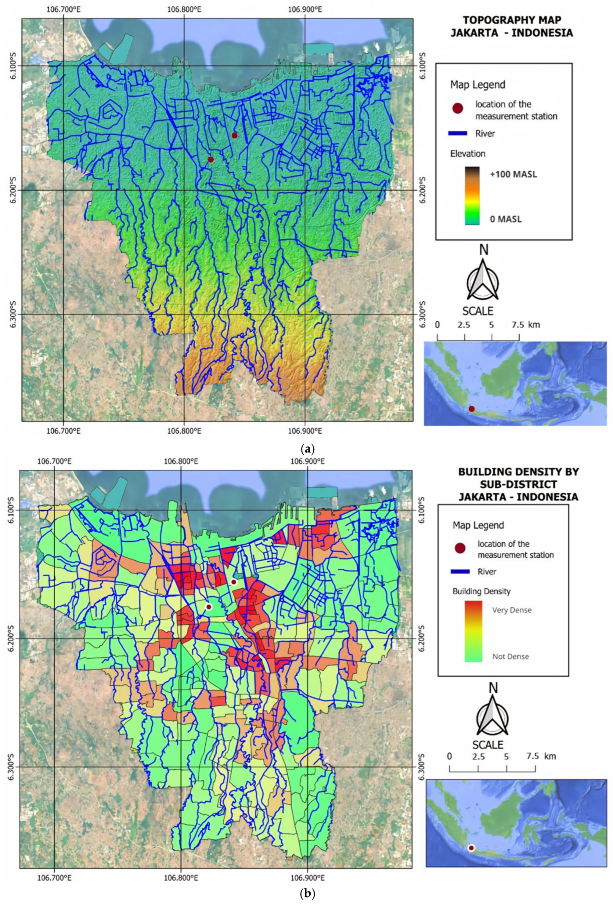
Jakarta is a megacity that has undergone rapid urbanization and expansion of built-up areas over the past decades. These changes have affected social and economic conditions and influenced the local climate, for instance, through urban heat island effects (UHI) [18]. High population density, infrastructure development, and changes in land cover can generate significant microclimatic variations, particularly affecting temperature and rainfall patterns. These factors provide an essential context for the analysis of long-term climate data. They may also contribute to potential inhomogeneities observed in meteorological time series from stations in the area. Figure 1 presents a map of Jakarta, showing the topography, river network, building density, and the location of the measurement stations, providing a visual overview of the study area.

The map shows the low-lying terrain and dense built-up areas that characterize the city, essential factors influencing local climate conditions. Jakarta has a tropical monsoon climate (Am, tropical monsoon according to the Köppen climate classification, which features a short dry season and high annual precipitation), characterized by two main seasons, namely the rainy season (October to April) and the dry season (May to September) [5]. Westerly monsoon winds and convective activity caused by surface heating influence rainfall patterns [19]. Meanwhile, due to urbanization, air temperature is influenced by the intensity of solar radiation, cloud cover, and the density and structure of buildings. Topographically, Jakarta is a low-lying area directly adjacent to the Java Sea, making it highly vulnerable to climate change, such as rising extreme temperatures, increased rainfall intensity, and flood risk. Global climatological phenomena such as El Niño and the Indian Ocean Dipole (IOD) influence Jakarta’s local climate variability [5]. The long-term trend of rising temperatures and fluctuating precipitation reflects an increasingly complex hydrometeorological risk [6]. Therefore, this region is strategic for study using a non-stationary statistical approach to predict future hydrometeorological trends.

2.2. Data Sources and Description

This research focuses on Jakarta and utilizes annual maximum monthly rainfall (mm) and air temperature (°C) data. The rainfall data (mm) used in this study are the annual maximum data from the total daily data in a month. In contrast, the air temperature data (°C) is the annual maximum data from the average daily data in a month. The data is time series data covering the period from 1864 to 2020. Data for 1864–1990 were obtained from the KNMI Jakarta-Kemayoran/Java station (−6.17° latitude, 106.82° longitude; elevation 7 m), which was part of the Royal Meteorological and Magnetic Institute during the Dutch colonial period and later integrated into the Indonesian meteorological system under BMG. We obtained the 1991–2020 data from the BMKG Kemayoran station (−6.16° latitude, 106.84° longitude; elevation 4 m). Although the data come from two different institutional sources, both stations sit in the same urban area with relatively similar environmental conditions, and the small elevation difference (3 m) is unlikely to affect climate measurements significantly. Measurements followed standard BMKG procedures using calibrated instruments, ensuring accuracy and reliability of the data [20].

The difference in data sources raises concerns regarding data homogeneity. The homogeneity test using [21] showed that rainfall data are homogeneous (p-value = 0.0671), while the test identified the air-temperature data as inhomogeneous (p-value = 0.0047). In general, inhomogeneities in climate data can arise from non-climatic factors such as station relocation, changes in instrumentation, observation procedures, or environmental modifications [22,23]. This condition is more likely to reflect the influence of climate and urbanization in Jakarta rather than artificial changes due to station relocation or instrument differences, considering that both stations sit in close spatial proximity and follow the same measurement standards [21]. Therefore, despite the identified inhomogeneity, the dataset represents the longest and reliable climate record for Jakarta.

This research uses the longest homogeneous record available for Jakarta (1864–2020) to maximize power to detect slow, structural changes in margins and dependence. WMO guidance recognizes the value of long, quality-controlled single-station series for climate analysis where spatial coverage is limited, provided researchers address metadata and homogeneity. Our case-study focus (i) isolates methodology and (ii) establishes a baseline that researchers can later extend to multi-site or higher-frequency datasets.

2.3. Methodology

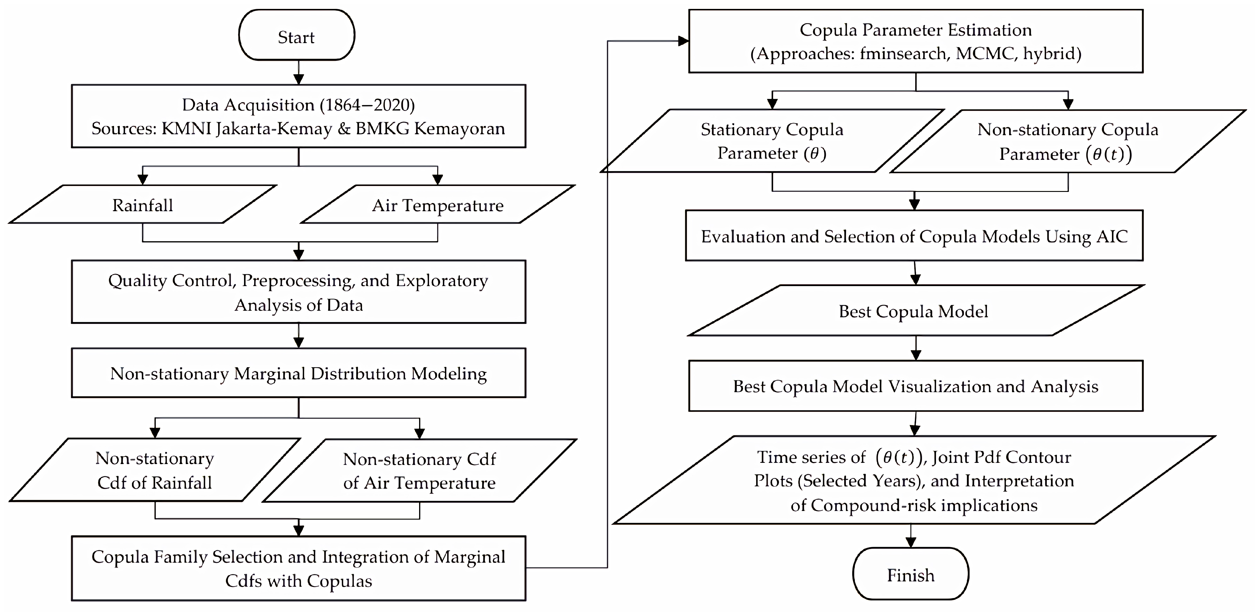
The Materials and Methods section presents the framework for analyzing Jakarta’s rainfall and air temperature extremes. To clarify, the overall workflow is summarized in Figure 2, offering a visual overview of the sequence of analysis steps.

2.3.1. Marginal Distributions

The marginal distributions of rainfall and air temperature were evaluated using probability density functions (pdf) and cumulative distribution functions (cdf) [24]. These functions were then extended to account for non-stationarity through time-varying distributions, where parameters change with time. In this study, a linear relationship was assumed for the location parameter:

$${\mu }_t=\left\{\begin{array}{cc}\mathrm{c}\mathrm{o}\mathrm{n}\mathrm{s}\mathrm{t}\mathrm{a}\mathrm{n}\mathrm{t},& \mathrm{i}\mathrm{f}\mathrm{s}\mathrm{t}\mathrm{a}\mathrm{t}\mathrm{i}\mathrm{o}\mathrm{n}\mathrm{a}\mathrm{r}\mathrm{y}\\ {\mu }_a+{\mu }_{b}t,& \mathrm{i}\mathrm{f}\mathrm{non-stationary}\end{array}\right.$$

(1)

where t is time; ${\mu }_a,{\mu }_b$ are new parameters for time-varying distributions.

The distribution used in this study results from research conducted by [16]. The research obtained the results of the non-stationary lognormal distribution with three parameters as the best distribution of rainfall data. The distribution comes from the cdf of the pdf. The following formula can obtain the pdf of the non-stationary lognormal distribution of rainfall random variables [25]:

$$f\left(x_1|\mu ,\sigma \right)={\displaystyle \frac{1}{x_1\sqrt{2\pi {\sigma }^2}}}\exp \left(-{\displaystyle \frac{{\left(\mathit{log}\left(x_1\right)-\left({\mu }_0+{\mu }_{1}t\right)\right)}^2}{{2\sigma }^2}}\right),x,\mu ,\sigma >0.$$

(2)

Like before, the GEV distribution is the best based on the research results of [16]. The research concluded that the non-stationary GEV distribution with four parameters is the best distribution of air temperature data. The cdf value of the pdf of the distribution was calculated. The following formula can obtain the pdf of a non-stationary lognormal distribution of rainfall random variables:

$$f\left(x_2|\mu ,\sigma ,\xi \right)=\left\{\begin{array}{cc}{\displaystyle \frac{1}{\sigma }}\exp \left(-\left(1+\xi {\left(a\right)}^{-{\displaystyle \frac{1}{\xi }}}\right)\right){\left[1+\xi \left(a\right)\right]}^{-{\displaystyle \frac{1}{\xi -1}}},& \xi \ne 0\\ {\displaystyle \frac{1}{\sigma }}\mathrm{e}\mathrm{x}\mathrm{p}\left(a\right)-\exp \left(a\right),& \xi =0\end{array}\right.$$

(3)

where $a={\displaystyle \frac{x_2-\left({\mu }_0+{\mu }_{1}t\right)}{\sigma }},-\mathbf{\infty }<x_2<\mathbf{\infty }$ [26]. The cdf of each distribution is obtained by integrating the pdf that has been obtained.

Equations (2) and (3) present the probability density functions of the non-stationary Lognormal distribution (for rainfall) and the non-stationary GEV distribution (for air temperature), respectively. In both models, the location parameter ${\mu }_0+{\mu }_{1}t$ varies linearly with time, while the scale parameter $\sigma >0$ controls the spread of the data and is assumed constant throughout the analysis period. A larger $\sigma$ indicates greater variability. For the GEV model, the shape parameter $\xi$ governs the tail behavior.

Alternative frameworks, such as the Metastatistical Extreme Value Distribution (MEVD) for daily rainfall extremes, have been shown to reduce sampling uncertainty and aid trend detection [27]. For temperature extremes, recent evaluations confirm the robustness of GEV—especially when combined with L-moments—while higher-parameter models like Wakeby may offer additional flexibility at the cost of increased complexity [28]. In this study, we retain Lognormal and GEV margins for comparability with prior Jakarta work and because they integrate cleanly with the copula framework applied here.

2.3.2. Copula Function

A bivariate copula is a bivariate distribution function $F\left(x_1,x_2\right)$ of random variables $X_1$ and $X_2$ with their marginal distribution functions $F_1\left(x_1\right)$ and $F_2\left(x_2\right)$ uniformly distributed i.e., $X_1,X_2~\mathrm{u}\mathrm{n}\mathrm{i}\mathrm{f}\mathrm{o}\mathrm{r}\mathrm{m}\left(0,1\right)$. According to Sklar’s theorem, any joint distribution function can be expressed in terms of its marginal distributions and a copula that captures the dependence structure:

$$F\left(x_1,x_2\right)=C\left(F_1\left(x_1\right),F_2\left(x_2\right)\right)=C\left(u,v\right)$$

(4)

where $F_1\left(x_1\right),F_2\left(x_2\right)$ are the marginal distributions of each random variable; $C\left(u,v\right)$ is the copula function [17].

This framework allows the separation between marginal behavior and the dependency structure, making copulas particularly useful for modeling nonlinear relationships in hydrometeorological variables. Among the various families, Archimedean copulas are widely applied because they provide the flexibility to capture both non-linear and extreme relationships in such data [29,30,31]. An Archimedean copula can be defined as follows:

$$C\left(u,v\right)={\phi }^{-1}\left[\phi \left(u\right)+\phi \left(v\right)\right],\forall u,v\in \left[0,1\right]$$

(5)

where $\phi$ is the copula generator function.

Prior research in Indonesia, such as the study by [32], applied rotated bivariate copulas (Clayton, Gumbel, BB-family) with the IFM method to model the joint distribution of the number of dry days and total precipitation in Southern Sumatra under various ENSO and IOD phases. They report significant dry-season dependence and shifts in joint density peaks under strong El Niño and favorable IOD conditions. This serves as a rationale for using Archimedean copulas in the present study to model the dependence structure between rainfall and temperature in Jakarta, with an additional focus on time-varying behavior.

The Archimedean copulas used in this study are the Clayton copula, the Gumbel copula, and the Frank copula. According to [30], Clayton, Gumbel, and Frank copulas are one-parameter Archimedean copulas representing various relationship patterns common in rainfall and air temperature data. Clayton copula is effective for modeling strong dependence in the lower tail (low extreme values), Gumbel copula for dependence in the upper tail (high extreme values), and Frank copula for symmetric relationships without dominance of either tail of the distribution. We prioritized one-parameter Archimedean copulas (Clayton, Gumbel, Frank) to balance parsimony, interpretability (clear tail focus), and sample-size constraints. With potentially weak to moderate dependence in annual maximum data, models with multiple shape parameters (e.g., BB1/BB7/Joe [33]) or alternative classes (e.g., t-copulas) risk identifiability and overfitting without clear information gain; AIC explicitly penalizes such added complexity. Our lower-tail interest is well captured by Clayton, while Gumbel and Frank span upper-tail and symmetric cases, covering the plausible regime space for this dataset. The general form of each Archimedean copula used is shown in Table 1 [17].

Table 1. General form of copula functions used.

Copula Name	General Form of Copula
Clayton copula	$C_{\mathrm{C}\mathrm{l}\mathrm{a}\mathrm{y}\mathrm{t}\mathrm{o}\mathrm{n}}\left(u,v;\theta \right)={\left(u^{-\theta }+v^{-\theta }-1\right)}^{-{\displaystyle \frac{1}{\theta }}},\theta \ge -1$	(6)
Gumbel copula	$C_{\mathrm{G}\mathrm{u}\mathrm{m}\mathrm{b}\mathrm{e}\mathrm{l}}\left(u,v;\theta \right)=e^{\left(-{\left[{\left(-\mathit{ln}u\right)}^{\theta }+{\left(-\mathit{ln}v\right)}^{\theta }\right]}^{{\displaystyle \frac{1}{\theta }}}\right)},\theta \ge 1$	(7)
Frank copula	$C_{\mathrm{F}\mathrm{r}\mathrm{a}\mathrm{n}\mathrm{k}}\left(u,v;\theta \right)=-{\displaystyle \frac{1}{\theta }}\ln \left(1+{\displaystyle \frac{\left(e^{-\theta u}-1\right)\left(e^{-\theta v}-1\right)}{e^{-\theta }-1}}\right),\theta =R-\left\{0\right\}$	(8)

Description: $u$ is the marginal cdf of rainfall data; and $v$ is the marginal cdf of air temperature.

Table 1. General form of copula functions used.

Copula Name	General Form of Copula
Clayton copula	$C_{\mathrm{C}\mathrm{l}\mathrm{a}\mathrm{y}\mathrm{t}\mathrm{o}\mathrm{n}}\left(u,v;\theta \right)={\left(u^{-\theta }+v^{-\theta }-1\right)}^{-{\displaystyle \frac{1}{\theta }}},\theta \ge -1$	(6)
Gumbel copula	$C_{\mathrm{G}\mathrm{u}\mathrm{m}\mathrm{b}\mathrm{e}\mathrm{l}}\left(u,v;\theta \right)=e^{\left(-{\left[{\left(-\mathit{ln}u\right)}^{\theta }+{\left(-\mathit{ln}v\right)}^{\theta }\right]}^{{\displaystyle \frac{1}{\theta }}}\right)},\theta \ge 1$	(7)
Frank copula	$C_{\mathrm{F}\mathrm{r}\mathrm{a}\mathrm{n}\mathrm{k}}\left(u,v;\theta \right)=-{\displaystyle \frac{1}{\theta }}\ln \left(1+{\displaystyle \frac{\left(e^{-\theta u}-1\right)\left(e^{-\theta v}-1\right)}{e^{-\theta }-1}}\right),\theta =R-\left\{0\right\}$	(8)

Description: $u$ is the marginal cdf of rainfall data; and $v$ is the marginal cdf of air temperature.

Beyond these static forms, this study also examines the possibility that the rainfall–temperature dependence evolves over time. Time-varying copula is a method that allows the dependency parameter $\theta$ between variables to change over time, providing flexibility for analyzing dynamic relationships in time series data [6,34]. In the non-stationary case, $\theta$ is modeled to vary linearly with time ${\theta }_t={\theta }_a+{\theta }_{b}t$.

2.3.3. Parameter Estimation

Copula parameter estimation is performed for stationary and non-stationary models using three approaches: (1) Maximum Likelihood Estimation (MLE) with the fminsearch algorithm, (2) Markov Chain Monte Carlo (MCMC) simulation, and (3) a combination of both. The complementary strengths of these methods make them suitable for estimating parameters from complex, potentially non-linear, time-varying dependence structures. The fminsearch algorithm [35] enables fast optimization of the log-likelihood function without requiring derivatives, making it suitable for simpler likelihood surfaces. MCMC methods [36,37,38], implemented here via the Metropolis–Hastings sampler, allow the exploration of posterior distributions and incorporate parameter uncertainty [39]. To interpret the posterior distribution, the histogram of the sample points is visualized and summary statistics (mean, median, and Maximum A Posteriori/MAP) are calculated. The choice of the final parameter estimate depends on the distribution shape: if the posterior is symmetric, the mean is used; if asymmetric or skewed, the median is preferred; and if a clear peak is present, the MAP value is taken as the parameter estimate. Combining both methods is expected to produce more robust and stable estimations, with fminsearch providing effective initial values to accelerate MCMC convergence. This hybrid approach will also likely reduce estimation bias and improve the reliability of capturing the dynamic dependence between rainfall and air temperature.

This approach is consistent with [32], who utilize rotated copulas and the Inference Function for-Margins (IFM) approach, testing multiple families and selecting the best fit via Cramér–von Mises statistics, to robustly capture tail dependence in joint temperature–precipitation variables. Meanwhile [40], models the relationship between total precipitation, the number of dry days, and hotspots in Kalimantan, Indonesia, for each ENSO phase using a nested 3-copula approach. These examples demonstrate the suitability of flexible copula-based estimation frameworks for complex, potentially non-linear dependence structures.

2.3.4. Selection of the Best Copula Model with Akaike Information Criterion (AIC)

According to [41], researchers widely use the Akaike Information Criterion (AIC) to select the best statistical model. This method, introduced by Akaike in 1978, balances model fit and complexity by penalizing the number of estimated parameters. Unlike other criteria such as the Bayesian Information Criterion (BIC), pure log-likelihood comparison, or traditional goodness-of-fit tests, AIC provides a trade-off between goodness of fit and model parsimony. This criterion makes it particularly suitable in hydrology and climate modeling, where overly complex models may overfit limited data, while overly simple models may fail to capture key dependencies.

In this study, AIC is employed to select the best copula model among stationary and non-stationary Archimedean copulas. The model with the smallest AIC value is considered the most appropriate representation of the dependence structure between rainfall and air temperature. The AIC value is calculated using the formula:

$$AIC=-2\ln \left(L\right)+2k$$

(9)

where $k$ is number of parameters estimated in the model; $L$ is model likelihood (the largest likelihood of the model against the data).

2.3.5. Visualization and Analysis of the Best Copula Model

Visualization of the relationship between rainfall and air temperature was carried out using the best copula model selected based on the AIC value. This visualization not only serves to illustrate the relationship between the two variables, but also captures the temporal dynamics of the dependency structure, such as shifts in the relationship pattern between the early and later periods.

The first stage of visualization was conducted through the time series of the dependency parameter $\theta \left(t\right)$, which shows the dynamics of changes in the strength of dependence between rainfall and air temperature over the observation period. This visualization allows the identification of specific periods with stronger or weaker dependence. Subsequently, the joint PDF contour plot, was used to describe the joint probability density of rainfall and air temperature in selected years. Through this plot, changes in the shape of the joint distribution can be observed over time, including indications of long-term shifts in the dependency pattern. Researchers further interpreted these visualizations to assess compound-event risks, offering insights into how concurrent rainfall and temperature extremes may evolve under changing climate conditions.

3. Results

3.1. Data Trends and Stationary

Descriptive statistical analysis was the initial step in understanding each variable’s value distribution.

Table 2. Descriptive statistics of the data.

Variable	Minimum	Maximum	Average	Standard Deviation
Rainfall	173.0	1068.9	443.6	166.5
Air temperature	26.1	29.9	27.7	0.9

summarizes the minimum, maximum, mean, and standard deviation values for annual maximum rainfall and air temperature in Jakarta over the period 1864–2020.

The minimum and maximum values of the rainfall variable show significant differences in annual rainfall in Jakarta, with an average value of around 443.6 mm per year. The high standard deviation indicates that rainfall experiences large fluctuations between years. On the other hand, annual air temperature has a narrower range of values, with a minimum value of 26.1 °C, a maximum of 29.9 °C, an average of 27.7 °C, and a standard deviation of 0.9 °C, reflecting that variations in annual air temperature tend to be more stable when compared to rainfall.

Figure 3 presents a regression graph of Jakarta’s rainfall and air temperature data over the period 1864–2020.

Based on the graph, it can be seen that both variables show a pattern that tends to increase over time.

To formally assess stationarity, the Kwiatkowski–Phillips–Schmidt–Shin (KPSS) test was applied [42,43]. The null hypothesis $\left(H_0\right)$ assumes that the data are stationary, while the alternative $\left(H_1\right)$ indicates non-stationarity. The significance level used is 5% with a critical value of 0.4630 [42]. If the KPSS statistic is below this threshold, $H_0$ cannot be rejected, indicating stationarity; otherwise, $H_0$ is rejected, indicating non-stationarity [44]. The results obtained are presented in

Table 3. KPSS test results of rainfall and air temperature variables.

Variable	KPSS Statistical Result	Critical Value	Decision
Rainfall	0.6567	0.4630	Reject H0
Air temperature	12.6616	0.4630	Reject H0

.

Based on the KPSS test results presented in Table 3, both series reject the null hypothesis of stationarity, indicating that rainfall and air temperature are non-stationary.

3.2. Marginal Distribution Modeling

Parameter estimation of marginal distributions for rainfall and air temperature was conducted using a non-stationary approach following [16]. The best-fitting distributions and their parameter values are shown in

Table 4. Parameter values of the best distribution results.

Variable	Distribution	Parameter Values
		$\widehat{\mathit{\mu }}$	$\widehat{\mathit{\sigma }}$	$\widehat{\mathit{\xi }}$
Rainfall	Lognormal	0.0014t + 5.9183	0.3631	-
Air temperature	GEV	0.0184t + 26.0970	0.3459	−0.1182

.

Based on Table 4, rainfall data is modeled using a lognormal distribution with a location parameter $\left(\widehat{\mu }\right)$ that changes linearly with time, namely $\widehat{\mu }\left(t\right)=0.0014\mathrm{t}+5.9183$, and a location parameter $\left(\widehat{\sigma }\right)$ of 0.3631. The air temperature data is modeled with a Generalized Extreme Value (GEV) distribution which also has a time-dependent location parameter, namely $\widehat{\mu }\left(t\right)=0.0184\mathrm{t}+26.0970$, as well as a scale parameter $\left(\widehat{\sigma }\right)$ of 0.3459 and a shape parameter $\left(\widehat{\xi }\right)$ of negative 0.1182.

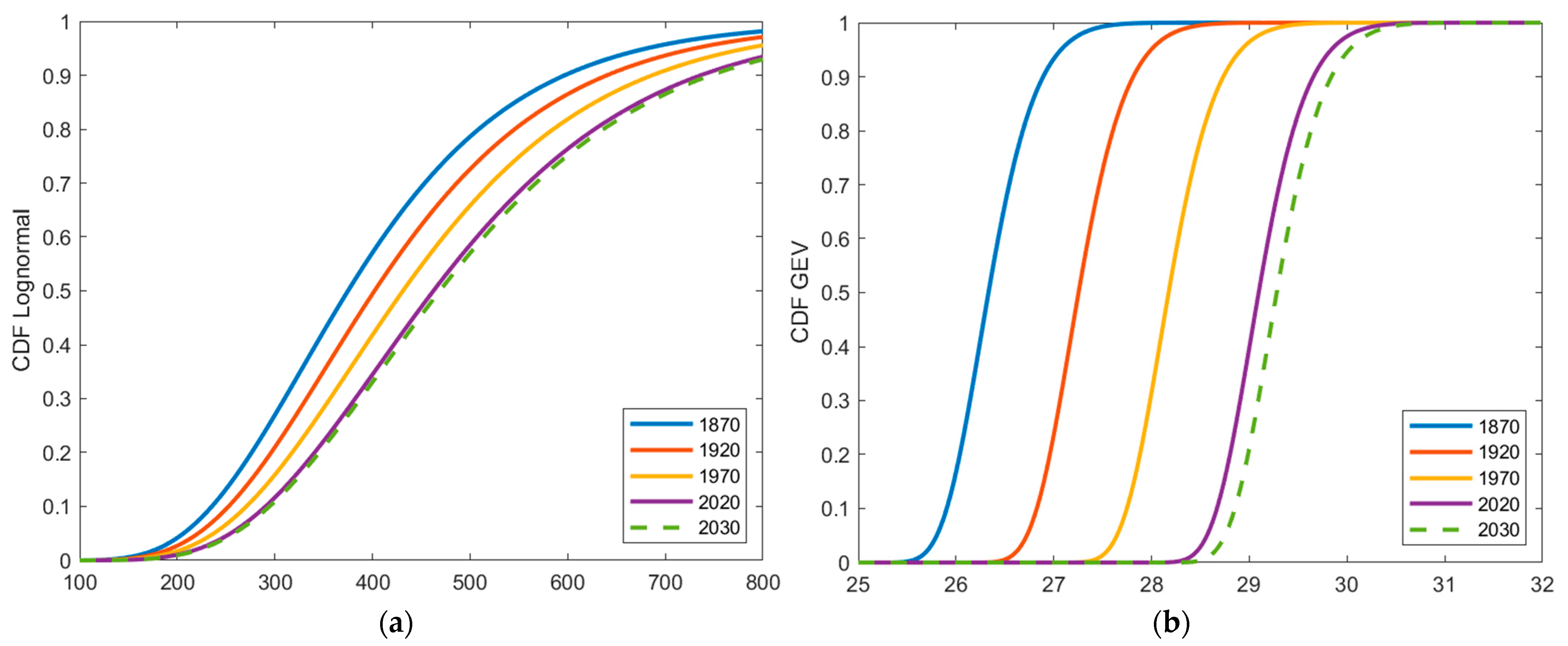
The fitted cumulative distribution functions of the annual maximum rainfall and air temperature data are presented in Figure 4.

There is a shift in the curve over time, which reflects changes in the distribution characteristics of both variables in the long term.

Cdf values are obtained from modeling results using the best distribution: Lognormal on rainfall data and GEV on air temperature data. The Kolmogorov–Smirnov (K-S) test evaluates the distribution of cdf values by comparing the empirical distribution to the uniform distribution (0,1). The K-S test uses a significance level of $\alpha =0.05$. The null hypothesis $\left(H_0\right)$ assumes that cdf value follows uniform distribution (0,1), while the alternative $\left(H_1\right)$ indicates not follow uniform distribution (0,1).

Table 5. K-S test results on cdf values of rainfall and air temperature.

Variable	p-Value	Decision
Rainfall	0.6812	Failed to reject $H_0$
Air temperature	0.5892	Failed to reject $H_0$

below presents a summary of the K-S test results on the cdf values of rainfall and air temperature.

Based on the K-S test, both p-value exceed the significance threshold, indicating that the fitted marginal distributions adequately follow a uniform distribution on (0,1).

3.3. Stationary Copula Parameter Estimation

3.3.1. Fminsearch Algorithm Approach

Parameter estimation using the fminsearch algorithm is based on the maximum likelihood method. Initial parameter values are set according to copula type: Clayton (−1), Gumbel (1), and Frank (real numbers near 0). Estimation assumes stationary dependence. The results of copula parameter estimation using the fminsearch algorithm (

Table 6. Stationary copula parameters with fminsearch algorithm approach.

Copula Name	$\mathbf{Parameter}\widehat{\mathit{\theta }}$ with Fmisearch Algorithm
Clayton copula	0.1418
Gumbel copula	1.0482
Frank copula	0.4540

).

Table 6 shows the parameter estimation results for each stationary copula using the fminsearch algorithm approach. The Clayton copula (0.1418) indicates weak positive dependence in the lower tail. The Gumbel copula (1.0482) indicates weak positive dependence in the upper tail. The Frank copula (0.4540) shows low positive dependence across the entire data range.

3.3.2. MCMC Simulation Approach

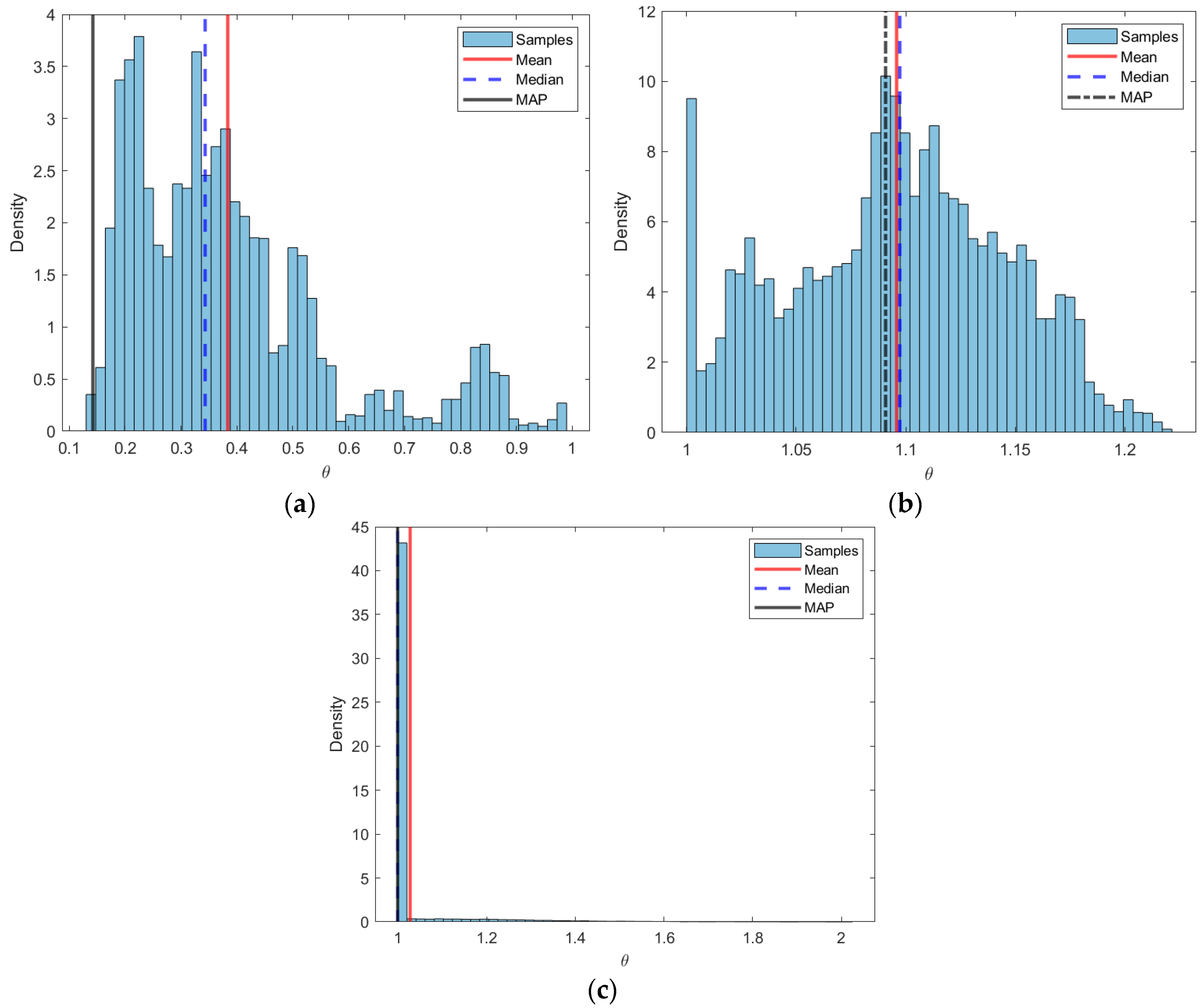
MCMC simulation estimates posterior distributions of copula parameters. Initial values follow the same rules as fminsearch. MCMC simulation results are presented as a graph illustrating the distribution and variability of the parameter estimates.

Table 7 below presents a numerical summary of the posterior parameter estimation results of the three copulas with the MCMC simulation approach, including the mean, median, and MAP values.

Based on Figure 5 and Table 7, Clayton posterior is right-skewed, so median (0.3430) chosen. Gumbel has a clear peak, so MAP (1.0910) chosen. Frank also peaked, so MAP (1.0000) chosen.

Table 7. Numerical summary of stationary copula parameters with MCMC.

Copula Name	Numerical Summary of Copula Parameter Estimation Results
	Mean	Median	MAP
Clayton copula	0.3840	0.3430 *	0.1420
Gumbel copula	1.0960	1.0970	1.0910 *
Frank copula	1.0280	1.0000	1.0000 *

* selected parameter values.

Table 7. Numerical summary of stationary copula parameters with MCMC.

Copula Name	Numerical Summary of Copula Parameter Estimation Results
	Mean	Median	MAP
Clayton copula	0.3840	0.3430 *	0.1420
Gumbel copula	1.0960	1.0970	1.0910 *
Frank copula	1.0280	1.0000	1.0000 *

* selected parameter values.

3.3.3. Combined Approach of Fminsearch-MMC on Stationary Copula

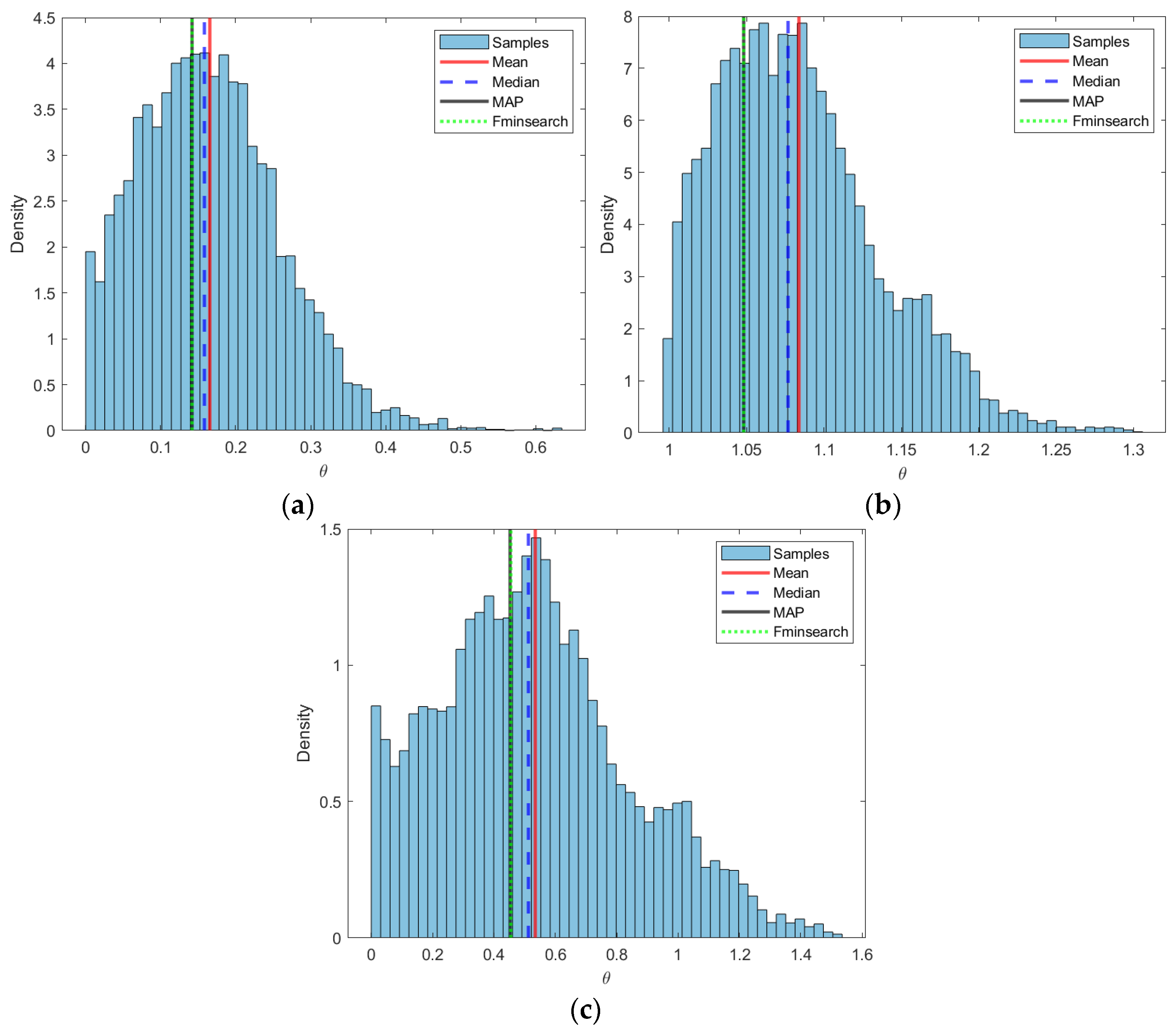
The fminsearch algorithm-MCMC simulation approach uses fminsearch estimates as initial values and refines them via MCMC. The parameter estimation results appear as a graph showing the distribution of parameter values.

Table 8 below presents a numerical summary of the posterior parameter estimation results of the three copulas with the fminsearch algorithm-MMC simulation approach, including the mean, median, and MAP values.

Based on Figure 6 and Table 8, distributions right-skewed, so median used for all copulas.

Table 8. Numerical summary of stationary copula parameters with fminsearch- MCMC.

Copula Name	Numerical Summary of Copula Parameter Estimation Results
	Mean	Median	MAP
Clayton copula	0.1654	0.1584 *	0.1421
Gumbel copula	1.0837	1.0770 *	1.0483
Frank copula	0.5334	0.5118 *	0.4535

* selected parameter values.

Table 8. Numerical summary of stationary copula parameters with fminsearch- MCMC.

Copula Name	Numerical Summary of Copula Parameter Estimation Results
	Mean	Median	MAP
Clayton copula	0.1654	0.1584 *	0.1421
Gumbel copula	1.0837	1.0770 *	1.0483
Frank copula	0.5334	0.5118 *	0.4535

* selected parameter values.

3.3.4. Summary of Stationary Parameter Estimation

Table 9. Parameter estimation results of stationary copulas.

Copula Name	$\mathbf{Parameter}\mathbf{Estimation}\mathbf{Results}\widehat{\mathit{\theta }}$
	Fminsearch	MCMC	Fminsearch-MCMC
Clayton copula	0.1418	0.3430	0.1584
Gumbel copula	1.0482	1.0910	1.0770
Frank copula	0.4540	1.0000	0.5118

below summarizes the parameter estimation results of the three stationary copulas based on the three approaches.

Based on Table 9, all copulas indicate weak dependence. The Clayton copula, being farther from its lower limit $\left(\theta =-1\right)$, better represents the dependence than the other copulas.

3.4. Non-Stationary Copula Parameter Estimation

The dependence parameter $\widehat{\theta }$ in the non-stationary copula is expressed as a linear function of time. The parameter is expressed as $\widehat{\theta }\left(t\right)={\widehat{\theta }}_{a}t+{\widehat{\theta }}_b$ with ${\widehat{\theta }}_a$ as the time variable coefficient and ${\widehat{\theta }}_b$ as a constant.

3.4.1. Fminsearch Algorithm Approach to Non-Stationary Copula

The fminsearch algorithm approach is applied to the non-stationary copula model to obtain maximum likelihood-based estimates of the dependence parameters. Clayton copula uses the initial value $\widehat{\theta }\left(t\right)=0t-1$. Gumbel copula uses an initial value of $\widehat{\theta }\left(t\right)=0t+1$. Frank copula uses an initial value of $\widehat{\theta }\left(t\right)\to 0t+0$. The results of copula parameter estimation using the fminsearch algorithm for the non-stationary model (

Table 10. Non-stationary copula parameters with the fminsearch algorithm.

Copula Name	$\mathbf{Copula}\mathbf{Parameter}\mathbf{Value}\widehat{\mathit{\theta }}\left(\mathit{t}\right) = {\widehat{\mathit{\theta }}}_{\mathit{a}}\mathit{t} + {\widehat{\mathit{\theta }}}_{\mathit{b}}$
Clayton copula	$0.0019t+0.1418$
Gumbel copula	$0.0003t+1.0178$
Frank copula	$0.0013t-1.6010$

).

The results indicate that all three copulas have a positive time coefficient, reflecting a gradual increase in dependence between rainfall and air temperature over time. The Clayton copula shows weak lower-tail dependence, the Gumbel copula exhibits weak upper-tail dependence, and the Frank copula shows weak dependence across the full distribution.

3.4.2. MCMC Simulation Approach on Non-Stationary Copula

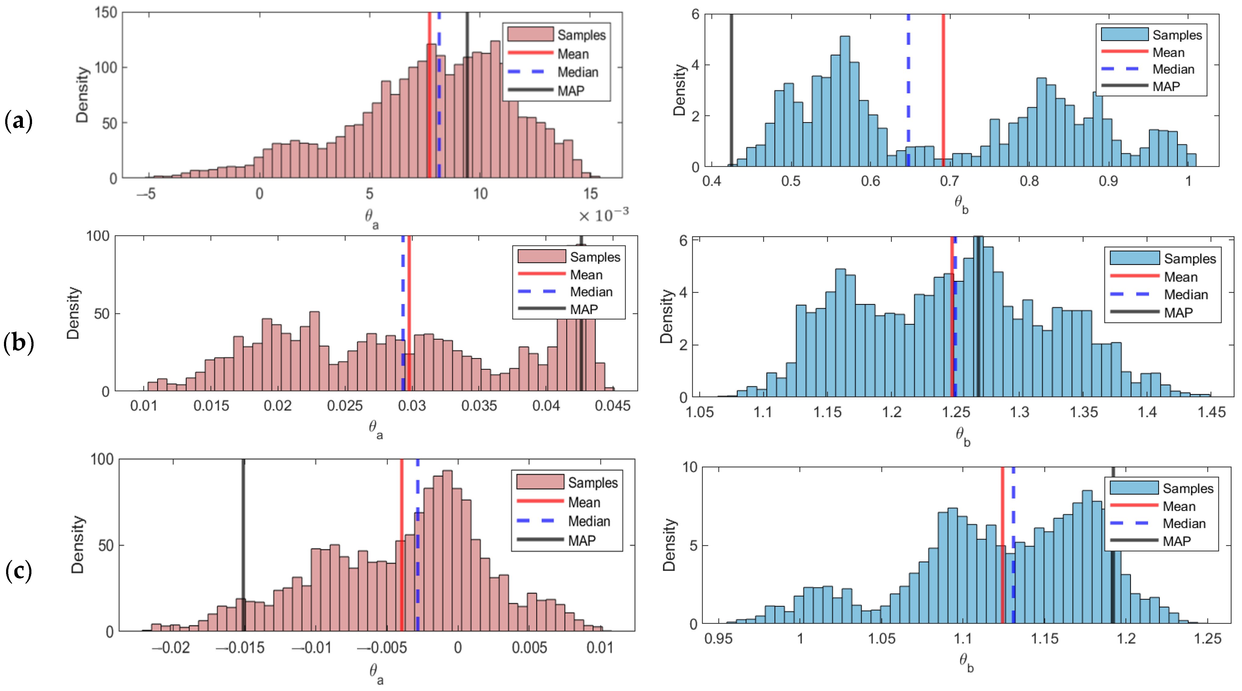
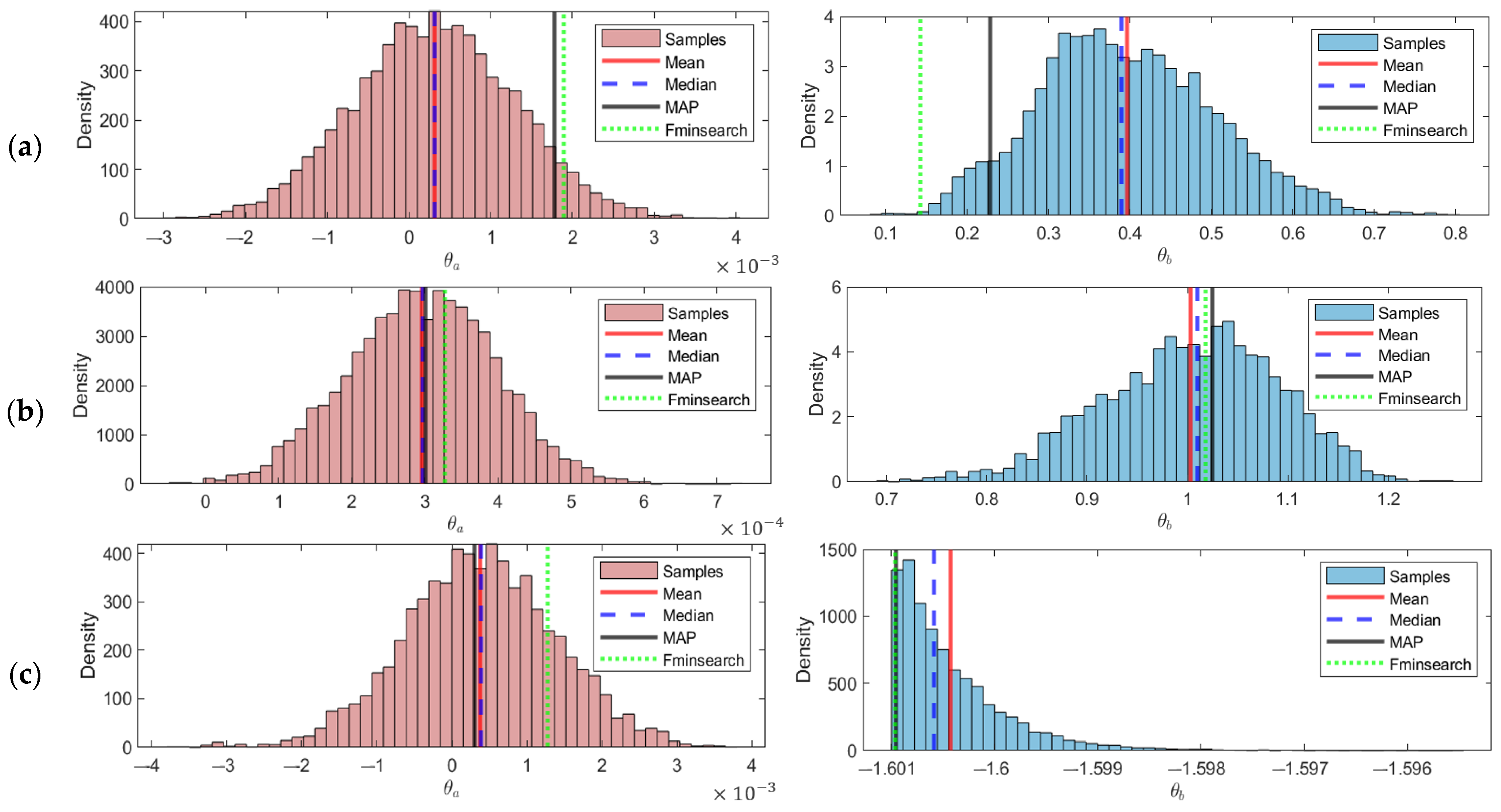
A MCMC simulation approach is used to obtain the parameter estimates of the non-stationary copula based on the posterior distribution results. Initial values follow the same rules as fminsearch. The results of parameter estimation through MCMC simulation are displayed in the form of two graphs for each copula, namely the distribution graph of the parameter value ${\widehat{\theta }}_a$ as the coefficient of the time variable and the graph of the parameter ${\widehat{\theta }}_b$ as a constant. These two graphs provide an overview of the distribution and variability of each parameter in the non-stationary copula model.

Table 11 below summarizes the posterior parameter estimation results (mean, median, and MAP values) of the three non-stationary copulas based on the MCMC simulation approach.

Figure 7 and Table 11 show the posterior distributions and numerical summaries of ${\widehat{\theta }}_a$ and ${\widehat{\theta }}_b$ for the three non-stationary copulas. The distribution of each parameter differs, which determines the choice of the most representative estimate. For the Clayton copula, the distribution of ${\widehat{\theta }}_a$ is left-skewed, so the median value of 0.0081 is selected, while ${\widehat{\theta }}_b$ shows a right-stretched distribution, leading to a median value of 0.6470. In the Gumbel copula, both ${\widehat{\theta }}_a$ and ${\widehat{\theta }}_b$ exhibit sharply peaked distributions, so the MAP values of 0.0426 and 1.2680 are chosen. For the Frank copula, ${\widehat{\theta }}_a$ has a left-skewed distribution, resulting in a median of −0.0029, and ${\widehat{\theta }}_b$ also extends to the left, giving a median value of 1.1310. These values indicate that time has a small positive contribution to increasing dependence in Clayton and Gumbel copulas, while Frank shows a slight decrease in dependence over time. Baseline dependence ${\widehat{\theta }}_b$ is moderate to strong in the lower and upper tails but weak across the full distribution.

Table 11. Numerical summary of non-stationary copula parameters with MCMC.

Copula Name	Numerical Summary of Copula Parameter Estimation Results
	${\widehat{\mathit{\theta }}}_{\mathit{a}}$ (Time Variable Coefficient)			${\widehat{\mathit{\theta }}}_{\mathit{b}}$ (Constant)
	Mean	Median	MAP	Mean	Median	MAP
Clayton copula	0.0077	0.0081 *	0.0094	0.6920	0.6470 *	0.4250
Gumbel copula	0.0298	0.0293	0.0426 *	1.2480	1.2500	1.2680 *
Frank copula	−0.0040	−0.0029 *	−0.0220	1.1240	1.1310 *	0.9570

* selected parameter values.

Table 11. Numerical summary of non-stationary copula parameters with MCMC.

Copula Name	Numerical Summary of Copula Parameter Estimation Results
	${\widehat{\mathit{\theta }}}_{\mathit{a}}$ (Time Variable Coefficient)			${\widehat{\mathit{\theta }}}_{\mathit{b}}$ (Constant)
	Mean	Median	MAP	Mean	Median	MAP
Clayton copula	0.0077	0.0081 *	0.0094	0.6920	0.6470 *	0.4250
Gumbel copula	0.0298	0.0293	0.0426 *	1.2480	1.2500	1.2680 *
Frank copula	−0.0040	−0.0029 *	−0.0220	1.1240	1.1310 *	0.9570

* selected parameter values.

3.4.3. Combined Fminsearch-MMC Approach to Non-Stationary Copula

The fminsearch algorithm-Markov Chain Monte Carlo (MCMC) simulation approach to non-stationary copula estimates the parameters of a non-stationary copula that combines two approaches. The primary estimation process of this method still uses MCMC simulation. Still, the initial parameter values come from the estimation results obtained through the fminsearch algorithm. The parameter estimation results from the fminsearch algorithm–MCMC simulation appear as two graphs for each copula.

Table 12 below presents a numerical summary of the posterior parameter estimation results of the three non-stationary copulas based on the MCMC fminsearch-simulation algorithm approach.

Figure 8 and show the combined fminsearch-MCMC results. The Clayton and Gumbel copulas exhibit mostly symmetric ${\widehat{\theta }}_a$, distributions, so mean values are selected, while ${\widehat{\theta }}_b$ shows slight skewness, leading to median selection. For Frank, ${\widehat{\theta }}_a$ is symmetric and ${\widehat{\theta }}_b$ slightly right-skewed, so mean and median are chosen, respectively. Overall, the combined approach produces stable estimates, with time having minimal positive effects on dependence in Clayton and Gumbel, and a weak effect in Frank.

Table 12. Numerical summary of nonstationary copula parameters with fminsearch-MCMC.

Copula Name	Numerical Summary of Copula Parameter Estimation Results
	${\widehat{\mathit{\theta }}}_{\mathit{a}}$ (Time Variable Coefficient)			${\widehat{\mathit{\theta }}}_{\mathit{b}}$ (Constant)
	Mean	Median	MAP	Mean	Median	MAP
Clayton copula	0.0003 *	0.0003	0.0018	0.3964	0.3893 *	0.2279
Gumbel copula	0.0003 *	0.0003	0.0003	1.0034	1.0095 *	1.0247
Frank copula	0.0004 *	0.0004	0.0003	−1.6004	−1.6006 *	−1.6010

* selected parameter values.

Table 12. Numerical summary of nonstationary copula parameters with fminsearch-MCMC.

Copula Name	Numerical Summary of Copula Parameter Estimation Results
	${\widehat{\mathit{\theta }}}_{\mathit{a}}$ (Time Variable Coefficient)			${\widehat{\mathit{\theta }}}_{\mathit{b}}$ (Constant)
	Mean	Median	MAP	Mean	Median	MAP
Clayton copula	0.0003 *	0.0003	0.0018	0.3964	0.3893 *	0.2279
Gumbel copula	0.0003 *	0.0003	0.0003	1.0034	1.0095 *	1.0247
Frank copula	0.0004 *	0.0004	0.0003	−1.6004	−1.6006 *	−1.6010

* selected parameter values.

3.4.4. Summary of Non-Stationary Parameter Estimation

Table 13. Parameter estimation results of non-stationary copulas.

Copula Name	$\mathbf{Parameter}\mathbf{Estimation}\mathbf{Results}\widehat{\mathit{\theta }}\left(\mathit{t}\right) = {\widehat{\mathit{\theta }}}_{\mathit{a}}\mathit{t} + {\widehat{\mathit{\theta }}}_{\mathit{b}}$
	Fminsearch	MCMC	Fminsearch-MCMC
Clayton copula	$0.0019t+0.1418$	$0.0019t+0.1418$	$0.0003t+0.3893$
Gumbel copula	$0.0003t+1.0178$	$0.0003t+1.0178$	$0.0003t+1.0095$
Frank copula	$0.0013t-1.6010$	$0.0013t-1.6010$	$0.0004t-1.6006$

below summarizes the parameter estimation results of the three non-stationary copulas based on the three approaches.

The results show that Clayton and Gumbel copulas exhibit increasing dependence over time at small rates, while Frank copula shows inconsistent patterns. The non-stationary Clayton copula better represents the dependency between rainfall and air temperature, with parameter values farther from the lower bound.

The results from the previous stationary model show that the relationship between rainfall and air temperature tends to be weak overall. However, the nonstationary approach reveals an increasing trend of dependence over time, although the values remain in the low range. This difference suggests that the nonstationary model can capture temporal dynamics that the stationary model cannot identify.

The increased dependence between air temperature and rainfall reflects a shift in climate dynamics in the study area. In tropical regions such as Jakarta, the dependence between these two variables previously tended to be weak and unstable. Still, the upward trend, although small, indicates that temperature changes are starting to have more impact on rainfall patterns, or vice versa. This phenomenon could be an early signal that Jakarta’s local climate system is beginning to experience changes in the interrelationships between climate elements, either due to anthropogenic factors such as global warming and urbanization, or natural factors such as seasonal variability. The increased dependency detected through the nonstationary model provides evidence that the hydrometeorological relationships in Jakarta are not static and require dynamic monitoring to adapt to and mitigate climate change in urban areas.

3.5. Selection and Visualization of the Best Copula Model

Comparing the AIC values of three copula types (Clayton, Gumbel, and Frank) using three estimation approaches (fminsearch, MCMC, and combination) identifies the best copula model. AIC was chosen as an evaluation measure because it can balance model complexity and estimation quality. A lower AIC value indicates a better model. The comparison results of the AIC values of the three copulas with stationary and non-stationary parameters are presented in

Table 14. AIC values of copula parameter estimation results.

Parameter Type	Copula Name	AIC Value
		Fminsearch	MCMC	Fminsearch-MCMC
Stationary	Clayton	4.3929	1.0650	0.4382 *
	Gumbel	2.9875	2.2760	2.5805
	Frank	2.9920	1.5620	1.4969
Nonstationary	Clayton	2.3929	−4.8690 *	0.2081
	Gumbel	2.7927	2.0000	2.7729
	Frank	2.5979	1.5100	1.3643

* lowest AIC value of each parameter type.

below.

Based on Table 14, the lowest AIC among stationary copulas is the Clayton copula estimated using the fminsearch-MCMC approach (0.4382). For non-stationary copulas, the lowest AIC is achieved by the Clayton copula estimated with the MCMC approach (−4.8690). Therefore, the non-stationary Clayton copula estimated using MCMC is selected as the best model in this study.

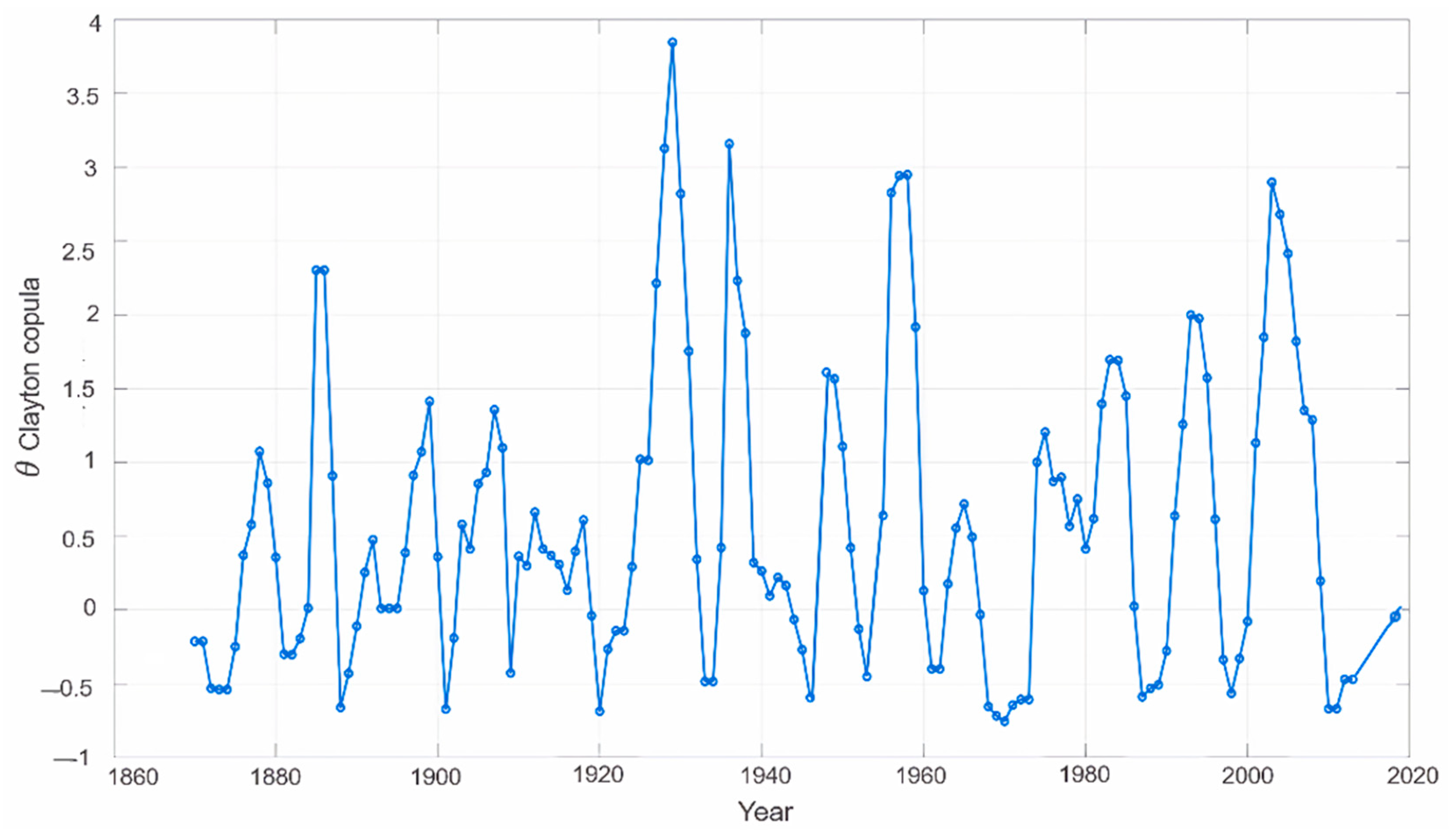
Figure 9 presents the time-series of the estimated θ(t) from the best non-stationary Clayton copula model. The $\theta \left(t\right)$ values reflect the time-varying dependence between rainfall and air temperature. Allowing $\theta$ to vary over time is central to our contribution, as it reveals temporal shifts in dependence that stationary copulas cannot capture. The results are presented in Figure 9.

Most values are positive, indicating a general positive dependence, but some years show slight decreases or temporary reversals. Even when average dependence is modest, these temporal shifts can meaningfully affect joint occurrence probabilities and compound-event risks, underscoring the importance of a time-varying copula framework.

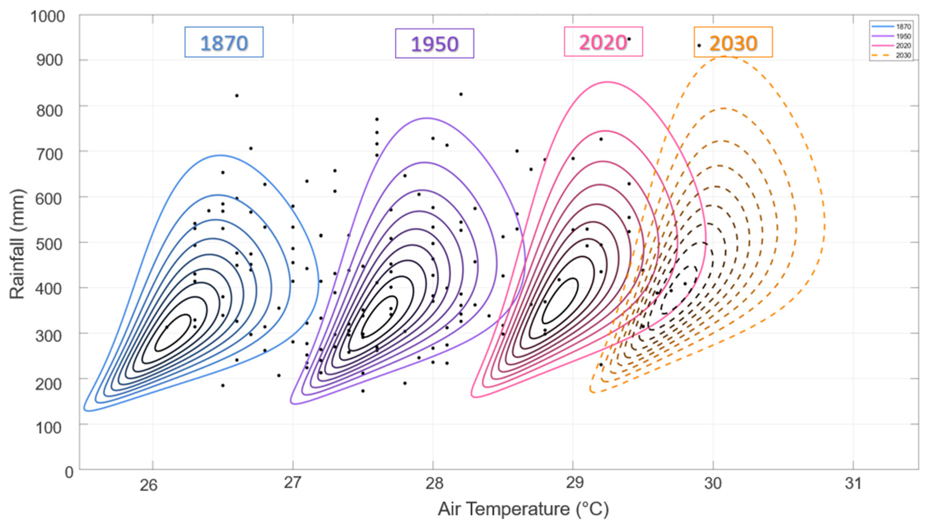
The contour plots in Figure 10 clearly illustrate how these dependencies change manifest at specific points in time. This visualization displays the joint distribution between rainfall and air temperature for several representative years. Each contour curve represents the shape and concentration of the probability of the most likely pairs of rainfall and temperature values for each period.

The contour plots show the temporal evolution of the joint distribution between air temperature and rainfall in Jakarta. Over time, the center of the distribution shifts toward higher temperatures and more variable rainfall. Projections for 2030 show a further shift towards higher temperatures, with still high rainfall but a flatter and more widespread distribution. This indicates increasing uncertainty over future rainfall values.

4. Discussion

4.1. Stationarity of Rainfall and Temperature

The KPSS results indicate that Jakarta’s rainfall and air temperature series are non-stationary, consistent with the graphical inspection, where both variables exhibit increasing long-term trends. According to [45], data series can be categorized as non-stationary if they show persistent upward or downward trajectories accompanied by fluctuations, a condition clearly observed in this study.

From a climatological perspective, the steady rise in annual air temperature reflects the intensification of global warming signals at the local scale. This finding is consistent with broader evidence of temperature increases across Indonesia and Southeast Asia over the past century, attributed to anthropogenic greenhouse gas emissions. In contrast, rainfall shows higher year-to-year variability with significant deviations from the mean, which may indicate enhanced climate variability. Such variability could increase the frequency of hydrometeorological extremes, including floods and droughts during dry years.

Researchers have documented similar non-stationarity in rainfall and temperature extremes in other tropical regions. For example [46], highlight that ENSO and IOD events strongly influence hydrometeorological extremes in Southeast Asia, which induce shifts in statistical properties over time. This external forcing complicates the assumption of stationarity and supports the application of time-varying models in climate risk analysis.

These results emphasize the methodological implications for modeling compound climate risks. If stationary models are applied, there is a risk of underestimating or misrepresenting long-term changes in rainfall–temperature dependence. By contrast, adopting non-stationary or time-varying copula approaches allows for a more accurate representation of evolving dependencies. This ensures that Jakarta’s climate adaptation and disaster risk management strategies rely on robust evidence.

4.2. Best-Fitting Marginal Distributions

The best-fitting marginal models were the Lognormal distribution for rainfall and the GEV distribution for air temperature. The time-dependent location parameters in both distributions indicate non-stationarity, consistent with the increasing trends observed in the raw series.

Researchers widely use the Lognormal distribution to model precipitation data for rainfall due to its positive support and ability to capture right-skewed behavior [25]. Its suitability for Jakarta reflects the substantial variability of annual maximum rainfall, consistent with findings in other tropical regions where rainfall distributions often deviate from symmetry. The GEV distribution has been consistently recommended for temperature in hydrological and climatological studies [26,28]. The negative shape parameter $(\xi <0)$ implies a bounded upper tail, suggesting that extreme annual maximum temperatures in Jakarta may have a natural upper limit. This is consistent with evaluations across Southeast Asia, where GEV margins robustly capture temperature extremes when combined with L-moment approaches [28].

The K-S test results confirm that the transformed cdf values follow a uniform distribution on (0,1), ensuring that the marginal models are statistically adequate. This validation step is essential before applying copula models, as copula theory requires well-fitted marginal distributions to capture dependence structures [17] accurately. These results highlight the necessity of accounting for time-varying characteristics in marginal distributions. A stationary assumption would ignore the shifting central tendencies of rainfall and temperature, potentially biasing subsequent dependence modeling. By adopting non-stationary Lognormal and GEV margins, the analysis provides a more realistic basis for copula-based joint modeling in Jakarta.

4.3. Stationary Copulas

The estimation results of the stationary copula parameters indicate that the relationship between rainfall and air temperature in Jakarta is positive but weak across all three copulas and estimation approaches. Differences in parameter values obtained through fminsearch, MCMC, and the combined fminsearch-MCMC reflect the characteristics of each method. For instance, the fminsearch approach provides more conservative initial estimates, often closer to the lower bound of the copula, while MCMC produces posterior distributions showing parameter variability and skewness. The combined fminsearch-MCMC approach leverages the strengths of both methods, producing stable estimates while accounting for posterior distribution characteristics.

The Clayton copula can better capture lower-tail dependence, which is relevant for low rainfall events accompanied by certain temperature conditions. Its parameter value, being farther from the lower bound than Gumbel and Frank, indicates that it more effectively represents the existing dependence, even if the intensity is weak. The Gumbel copula, focusing on upper-tail reliance, and the Frank copula, which captures dependence across the entire distribution, provide additional insight into the non-linear relationship between the two variables, although both also show low intensity.

This weak dependence between rainfall and air temperature may imply that the relationship between the two variables is non-linear and influenced by complex external factors. In tropical regions such as Indonesia, this phenomenon may be due to the influence of seasonal climate variability, such as El Niño and IOD, and local atmospheric dynamics that can trigger rainfall anomalies without significant temperature changes, or vice versa. Therefore, even if the statistical relationship is weak, it is still important to model it appropriately to understand the hydrometeorological dynamics in urban areas such as Jakarta. Unlike univariate designs, moderate dependence can substantially alter joint occurrence probabilities and compound return periods. Copulas (i) quantify tail-specific co-behavior (e.g., Clayton’s lower tail) that univariate fits cannot see, (ii) enable AND/OR/Kendall definitions of joint risk, and (iii) reveal time-variation in dependence $\left(\theta \right(t\left)\right)$ that may amplify compound hazards even when average $\tau$ is small. These are key for compound-event planning (e.g., dry–cool or hot–wet combinations). Recent reviews highlight that compound-event research benefits from large-ensemble simulations to assess low-probability robust but high-impact joint extremes [47]. In addition, new dependence metrics demonstrate that the tails of joint extremes (e.g., precipitation–wind or rainfall–temperature) may exhibit distinct behaviors critical for risk assessment [48]. These studies reinforce our use of copula-based approaches to better capture tail-specific dependence and compound-event relevance.

4.4. Non-Stationary Copulas

The non-stationary copula parameter estimation results indicate that Jakarta’s relationship between rainfall and air temperature exhibits an increasing trend over time, although the dependence values remain low. This contrasts with the stationary model, which captures only a fixed and generally weak dependence. This difference highlights that the non-stationary model can represent temporal dynamics in the interaction between climate variables that a stationary approach cannot capture.

The Clayton and Gumbel copulas show a small but positive contribution of time to the increasing dependence in the lower-tail and upper-tail distributions, respectively. In contrast, the Frank copula indicates a slight decrease in dependence across the full distribution. These findings suggest that, although the overall relationship is weak, temperature changes are beginning to influence rainfall patterns, or vice versa. This is consistent with tropical climate dynamics, where the rainfall–temperature relationship is complex and affected by seasonal variability, phenomena such as El Niño and IOD, and local atmospheric dynamics [47,48].

The upward trend in dependence detected by the non-stationary model has important implications for hydrometeorological monitoring and climate change risk mitigation in urban areas. The observed increase may be an early signal of shifts in Jakarta’s local climate system, driven by anthropogenic factors such as global warming, urbanization, and natural factors [47,48]. Therefore, non-stationary modeling provides a more realistic representation of the interaction between rainfall and temperature and supports dynamic planning for compound-event management and hydrometeorological risk [48].

4.5. Hydrometeorological Implications of the Selected Copula Model

The model selection results indicate that the non-stationary Clayton copula estimated using the MCMC approach is the best model to describe the dependence between rainfall and air temperature in Jakarta, as supported by the lowest AIC value compared to the other models. As reflected in the $\theta \left(t\right)$ values, the time-varying dependence confirms that the relationship between rainfall and air temperature is dynamic and not constant throughout the observation period. Although the average dependence is moderate, these fluctuations are vital because they affect the probabilities of joint occurrences, which a stationary copula cannot capture.

The $\theta \left(t\right)$ values are mostly positive, indicating a general positive dependence, although researchers observe slight decreases or temporary reversals in some years. Even when the average dependence is modest, these temporal shifts can significantly impact joint occurrence probabilities and compound-event risks, underscoring the importance of a time-varying copula framework. The distribution of $\theta \left(t\right)$ also confirms strong lower-tail dependence, particularly under low rainfall and low temperature conditions, as reflected by the selection of the Clayton copula. This pattern indicates that dry-cool conditions were still dominant in the early observation period and began to shift gradually over time. In other words, the non-stationary model is not only statistically valid but also relevant for capturing the dynamics of climate change in the lower extremes, which are not visible in stationary models.

These results relate to the contour visualizations and the latest temporal trends. Changing trends indicate significant impacts of hydrometeorological dynamics. The consistent rise in temperature reflects global warming, while the widening rainfall distribution signals increasing uncertainty and the risk of extreme events. The finding that the Clayton copula provides the best fit indicates strong lower-tail dependence, namely low-rainfall conditions that tend to coincide with low temperatures. Climatologically, this dependence structure implies that the frequency of low-temperature droughts—which often emerge at the beginning or end of the dry season in tropical regions—may increase. Such conditions can exacerbate water scarcity and reduce soil moisture availability, affecting the agricultural sector and urban water security. Conversely, the widening rainfall distribution and sustained temperature rise also suggest a higher potential for short, high-intensity rainfall events that may trigger urban flooding. Thus, these results demonstrate a statistical relationship and carry tangible implications for the increasing frequency of extreme events in the form of droughts and floods, consistent with the literature on compound climate extremes [49,50]. Studies in Indonesia also support these findings: [51] confirmed the influence of ENSO on droughts in Borneo using a copula approach. At the same time [52], showed a shift toward dry–dry conditions during strong El Niño and positive IOD phases in Southern Sumatra. These regional climatic linkages reinforce the relevance of the present findings, highlighting that Jakarta faces increasingly complex compound-event risks under climate change.

Our analysis indicates weak-to-moderate average dependence between Jakarta’s annual-maximum rainfall and air temperature. Yet, AIC consistently favors the time-varying Clayton copula and reveals lower-tail co-variability. Even when rank dependence is modest, compound-risk literature shows that tail-focused dependence can materially shift joint return periods, underscoring the value of a bivariate approach over separate univariate analyses. This aligns with recent compound-event studies emphasizing tail metrics and multivariate risk framing [48]. The finding that a lower-tail–sensitive copula best describes Jakarta is climatologically plausible. Jakarta has documented urban warming and a rapid expansion of built-up areas in recent decades, reshaping the surface energy balance and atmospheric stability. Such changes can alter the co-occurrence structure of temperature and rainfall extremes, including dry-cool combinations that matter for water supply and heat-stress transitions. Recent modeling and observational studies over Jakarta link LULC change with rising urban temperatures and evolving rainfall/thermal patterns, providing context for the slow drift we infer in $\theta \left(t\right)$ [53].

The contour shapes drawn to the lower left in the early years indicate that the strong dependence between low temperature and low rainfall is still dominant in that period, and starts to change gradually over time. Thus, the non-stationary Clayton copula is not only statistically valid, but also relevant for capturing the dynamics of climate change in the lower extremes that other models, including stationary ones, do not see. Methodologically, our pairing of non-stationary margins with a time-varying copula follows the broader move from stationary design assumptions to dynamic multivariate frameworks. The copula approach isolates the dependence structure from the marginals, supports alternative joint-risk definitions (AND/OR/Kendall), and cleanly accommodates parameter dynamics $\left(\theta \right(t\left)\right)$. While more flexible families exist, using one-parameter Archimedean copulas balances parsimony and interpretability given weak dependence and sample size; this echoes guidance in the hydrologic copula literature [54]. The 2030 projections show an increase in temperature and a widening distribution of rainfall, reflecting uncertainty and increasingly complex hydrometeorological risks in the future.

Finally, our results are consistent with univariate EVT insights: GEV-type models (for temperature) often provide robust extreme quantiles across sample sizes, and recent rainfall-extreme frameworks (e.g., MEVD) emphasize uncertainty minimization—both reinforcing the need to carry margin uncertainty into joint-risk estimation. Detecting the dependence between rainfall and temperature has important practical significance, as it suggests that extreme weather events in Jakarta are likely influenced by interactions among hydrometeorological components, rather than by a single variable, thus requiring an integrated response. The patterns projected for 2030 indicate increasing challenges in managing hydrometeorological disaster risks. Therefore, this insight supports the development of climate adaptation strategies that account for compound risks. Understanding this dependence can also strengthen early warning systems and improve scenario planning. These findings may also inform spatial planning policies and the development of resilient infrastructure in Jakarta in response to changing hydrometeorological conditions.

5. Conclusions

Selection of the best copula model based on the AIC value shows that the non-stationary Clayton copula with MCMC simulation estimation is the most suitable, as it produces the lowest AIC. The Clayton copula can represent the relationship between rainfall and air temperature in the lower tail of the distribution over time.

Visualization using the non-stationary Clayton copula with MCMC shows a time-varying relationship of temperature and rainfall, with an increasing trend in temperature and rainfall variation. Using a Clayton copula sensitive to the lower extremes allows the identification of potential low-temperature droughts. These results show that the non-stationary copula model effectively represents and predicts changes in hydrometeorological patterns in Jakarta.

The model developed in this study can serve as a foundation for policymakers in Jakarta to strengthen early warning systems for hydrometeorological risks, particularly in predicting the potential for drought, extreme rainfall, and extreme temperatures. These findings also support formulating mitigation strategies, spatial planning policies, and infrastructure development based on hydrometeorological risk.

This study has several limitations. First, the historical climate data used—particularly for early periods such as 1870—may contain uncertainties due to limited measurement coverage and quality. Second, inhomogeneity detected in the temperature series (Pettitt test, p = 0.0047) may reflect genuine climatic/urbanization influences rather than artificial breaks, given the close spatial setting and standardized instrumentation. Nevertheless, researchers should take this limitation into account when interpreting the results. Expanding the analysis to multi-site data would be a natural next step for future research. Third, using a single-parameter Archimedean copula may not capture all asymmetries or regime shifts in the data. Future studies could explore more affluent copula families if multi-site or higher-frequency data become available. Fourth, the non-stationary models assume a linear parameter evolution trend, simplifying the complex nature of climate variability. Finally, future projections are based on extrapolated copula behavior rather than dynamically linked climate models, such as General Circulation Models (GCMs), limiting predictive robustness over longer time horizons. The future 2030 projections presented here are extrapolated from the time-varying $\theta \left(t\right)$ values from the non-stationary Clayton copula, rather than dynamically linked climate models such as CMIP6. While this approach may limit predictive precision for longer horizons, it remains sufficient to capture temporal dependence trends and extreme event dynamics relevant for Jakarta.

Future research should explore more complex copula families, including multi-parameter and asymmetric copulas, to capture nonlinear and climate indicator-dependent dependencies more accurately. Future work in Jakarta could expand to multi-site or higher-frequency data, test more affluent copula families warranted by information criteria, and include covariate-driven dependence (e.g., ENSO/IOD, urban growth metrics) [27,28]. The results of this study indicate a relatively weak dependence between variables; therefore, the use of copulas with weak dependence characteristics, such as the Ali-Mikhail-Haq (AMH) copula, or nested copula structures, should also be considered, as they may offer greater flexibility. In addition, integrating data from GCMs and downscaled regional hydrometeorological projections could improve the accuracy of long-term predictions. Researchers can also extend this approach to other urban areas in Indonesia vulnerable to changes in hydrometeorological trends, thereby contributing more broadly to developing national- and international-scale climate models.

References

1. Ariska, M.; Akhsan, H.; Muslim, M.; Romadoni, M.; Putriyani, F.S. Prediksi perubahan iklim ekstrem di kota Palembang dan kaitannya dengan fenomena El Niño–Southern Oscillation (ENSO) berbasis machine learning. JIPFRI J. Inov. Pendidik. Fis. Ris. Ilm. 2022, 6, 79–86. [Google Scholar] [CrossRef]
2. Subiyanto, A.; Triutomo, S.; Wahyuni, D. Pengaruh perubahan iklim terhadap bencana hidrometeorologi di Kecamatan Cisarua-Kabupaten Bogor. PENDIPA J. Sci. Educ. 2022, 6, 541–546. [Google Scholar]
3. Intergovernmental Panel on Climate Change. Climate Change 2022: Impacts, Adaptation, and Vulnerability. Contribution of Working Group II to the Sixth Assessment Report of the Intergovernmental Panel on Climate Change; Pörtner, H.-O., Roberts, D.C., Tignor, M., Poloczanska, E.S., Mintenbeck, K., Alegría, A., Craig, M., Langsdorf, S., Löschke, V., Möller, A., et al., Eds.; Cambridge University Press: Cambridge, UK, 2022; in press. [Google Scholar]
4. Rahayu, H.P.; Haigh, R.; Amaratunga, D.; Kombaitan, B.; Khoirunnisa, D.; Pradana, V. A micro scale study of climate change adaptation and disaster risk reduction in coastal urban strategic planning for the Jakarta. Int. J. Disaster Resil. Built Environ. 2020, 11, 119–133. [Google Scholar] [CrossRef]
5. Jannah, M.; Sujono, J.; Raharjdo, A.P. Kajian perubahan iklim di DKI Jakarta berdasarkan data curah hujan. Teknisia 2023, 28, 43–54. [Google Scholar] [CrossRef]
6. Xu, P.; Wang, D.; Wang, Y.; Qiu, J.; Singh, V.P.; Ju, X.; Zhang, C. Time-varying copula and average annual reliability-based nonstationary hazard assessment of extreme rainfall events. J. Hydrol. 2021, 603, 126792. [Google Scholar] [CrossRef]
7. Chen, H.; Sun, J. Contribution of human influence to increased daily precipitation extremes over China. Geophys. Res. Lett. 2017, 44, 2436–2444. [Google Scholar] [CrossRef]
8. Call, B.C.; Belmont, P.; Schmidt, J.C.; Wilcock, P.R. Changes in floodplain inundation under nonstationary hydrology for an adjustable, alluvial river channel. Water Resour. Res. 2017, 53, 3811–3834. [Google Scholar] [CrossRef]
9. Ghanbari, M.; Arabi, M.; Obeysekera, J.; Sweet, W. A coherent statistical model for coastal flood frequency analysis under nonstationary sea level conditions. Earth’s Future 2019, 7, 162–177. [Google Scholar] [CrossRef]
10. Zhang, Q.; Gu, X.; Singh, V.P.; Chen, X. Evaluation of ecological instream flow using multiple ecological indicators with consideration of hydrological alterations. J. Hydrol. 2015, 529, 711–722. [Google Scholar] [CrossRef]
11. Ganguli, P.; Coulibaly, P. Does nonstationarity in rainfall require nonstationary intensity–duration–frequency curves? Hydrol. Earth Syst. Sci. 2017, 21, 6461–6483. [Google Scholar] [CrossRef]
12. Agilan, V.; Umamahesh, N.V. Covariate and parameter uncertainty in non-stationary rainfall IDF curve. Int. J. Climatol. 2018, 38, 365–383. [Google Scholar] [CrossRef]
13. Tian, Q.; Li, Z.; Sun, X. Frequency analysis of precipitation extremes under a changing climate: A case study in Heihe River basin, China. J. Water Clim. Change 2021, 12, 772–786. [Google Scholar] [CrossRef]
14. Yılmaz, M.; Tosunoğlu, F. Non-stationary low flow frequency analysis under climate change. Theor. Appl. Climatol. 2024, 155, 7479–7497. [Google Scholar] [CrossRef]
15. Rahmayani, D.; Sutikno, S. Analisis curah hujan ekstrim non-stasioner dengan pendekatan block maxima di Surabaya dan Mojokerto. J. Sains Seni ITS 2020, 8, D161–D168. [Google Scholar] [CrossRef]
16. Setyawati, S.N.; Nurdiati, S.; Mangku, I.W.; Najib, M.K. Time-varying distribution analysis for rainfall and air temperature data in Jakarta in response to future climate change. CAUCHY. in press.
17. Nelsen, R.B. An Introduction to Copulas; Springer: New York, NY, USA, 2006. [Google Scholar]
18. Fajary, F.R.; Lee, H.S.; Kubota, T.; Bhanage, V.; Pradana, R.P.; Nimiya, H.; Putra, I.D.G.A. Comprehensive spatiotemporal evaluation of urban growth, surface urban heat island, and urban thermal conditions on Java Island of Indonesia and implications for urban planning. Heliyon 2024, 10, 13. [Google Scholar] [CrossRef]
19. Sharafati, A.; Pezeshki, E. A strategy to assess the uncertainty of a climate change impact on extreme hydrological events in the semi-arid Dehbar catchment in Iran. Theor. Appl. Climatol. 2020, 139, 389–402. [Google Scholar] [CrossRef]
20. Badan Meteorologi, Klimatologi, Dan Geofisika (BMKG). Pedoman Pengamatan Meteorologi; BMKG: Jakarta, Indonesia, 2020.
21. Pettitt, A.N. A non-parametric approach to the change-point problem. Appl. Stat. 1979, 28, 126–135. [Google Scholar] [CrossRef]
22. Peterson, T.C.; Easterling, D.R.; Karl, T.R.; Groisman, P.; Nicholls, N.; Plummer, N.; Torok, S.; Auer, I.; Boehm, R.; Gullett, D.; et al. Homogeneity adjustments of in situ atmospheric climate data: A review. Int. J. Climatol. 1998, 18, 1493–1517. [Google Scholar] [CrossRef]
23. Wijngaard, J.B.; Klein Tank, A.M.G.; Können, G.P. Homogeneity of 20th century European daily temperature and precipitation series. Int. J. Climatol. 2003, 23, 679–692. [Google Scholar] [CrossRef]
24. Wasserman, L. All of Statistics: A Concise Course in Statistical Inference; Springer Science & Business Media: New York, NY, USA, 2004. [Google Scholar]
25. Crow, E.L.; Shimizu, K. Lognormal Distributions: Theory and Applications; Marcel Dekker: New York, NY, USA, 1988. [Google Scholar]
26. Coles, S.; Bawa, J.; Trenner, L.; Dorazio, P. An Introduction to Statistical Modeling of Extreme Values; Springer: London, UK, 2001; Volume 208, p. 208. [Google Scholar]
27. Miniussi, A.; Marani, M. Estimation of daily rainfall extremes through the metastatistical extreme value distribution: Uncertainty minimization and implications for trend detection. Water Resour. Res. 2020, 56, e2019WR026535. [Google Scholar] [CrossRef]
28. Anghel, C.G.; Ianculescu, D. Application of the GEV distribution in flood frequency analysis in Romania: An in-depth analysis. Climate 2025, 13, 152. [Google Scholar] [CrossRef]
29. Zhang, L.; Singh, V.P. Bivariate rainfall frequency distributions using Archimedean copulas. J. Hydrol. 2007, 332, 93–109. [Google Scholar] [CrossRef]
30. Tencer, B.; Weaver, A.; Zwiers, F. Joint occurrence of daily temperature and precipitation extreme events over Canada. J. Appl. Meteorol. Climatol. 2014, 53, 2148–2162. [Google Scholar] [CrossRef]
31. Bezak, N.; Zabret, K.; Šraj, M. Application of copula functions for rainfall interception modelling. Water 2018, 10, 995. [Google Scholar] [CrossRef]
32. Nurdiati, S.; Najib, M.K.; Thalib, A.S. Joint distribution and coincidence probability of the number of dry days and the total amount of precipitation in southern Sumatra fire-prone area. Geogr. Tech. 2022, 17, 107–118. [Google Scholar] [CrossRef]
33. Nikoloulopoulos, A.K.; Joe, H.; Li, H. Vine copulas with asymmetric tail dependence and applications to financial return data. Comput. Stat. Data Anal. 2012, 56, 3659–3673. [Google Scholar] [CrossRef]
34. Kiesel, R.; Mroz, M.; Stadtmueller, U. Time-varying copula models for financial time series. Adv. Appl. Probab. 2016, 48, 159–180. [Google Scholar] [CrossRef]
35. Mas’oed, T.W.; Nurdiati, S.; Sopaheluwakan, A.; Najib, M.K.; Salsabila, A. Modeling fire hotspots in Kalimantan, Indonesia, using nested 3-copula regression based on precipitation and dry days during different ENSO phases. Geogr. Tech. 2024, 19, 264–281. [Google Scholar] [CrossRef]
36. Lagarias, J.C.; Reeds, J.A.; Wright, M.H.; Wright, P.E. Convergence properties of the Nelder--Mead simplex method in low dimensions. SIAM J. Optim. 1998, 9, 112–147. [Google Scholar] [CrossRef]
37. Casella, G.; Berger, R. Statistical Inference; Chapman and Hall/CRC: Boca Raton, FL, USA, 2024. [Google Scholar]
38. Gamerman, D.; Lopes, H.F. Markov Chain Monte Carlo: Stochastic Simulation for Bayesian Inference; Chapman and Hall/CRC: Boca Raton, FL, USA, 2006. [Google Scholar]
39. Brooks, S.; Gelman, A.; Jones, G.; Meng, X.L. (Eds.) Handbook of Markov Chain Monte Carlo; CRC Press: Boca Raton, FL, USA, 2011. [Google Scholar]
40. Chen, T.; Morris, J.; Martin, E. Gaussian process regression for multivariate spectroscopic calibration. Chemom. Intell. Lab. Syst. 2007, 87, 59–71. [Google Scholar] [CrossRef]
41. Grasa, A.A. Econometric Model Selection: A New Approach; Springer Science & Business Media: New York, NY, USA, 2013; Volume 16. [Google Scholar]
42. Kwiatkowski, D.; Phillips, P.C.; Schmidt, P.; Shin, Y. Testing the null hypothesis of stationarity against the alternative of a unit root: How sure are we that economic time series have a unit root? J. Econom. 1992, 54, 159–178. [Google Scholar] [CrossRef]
43. Shin, Y.; Schmidt, P. A KPSS stationarity test as a unit root test. Econ. Lett. 1992, 38, 387–392. [Google Scholar] [CrossRef]
44. Zivot, E.; Wang, J. Modeling Financial Time Series with S-PLUS, 2nd ed.; Springer: New York, NY, USA, 2006. [Google Scholar]
45. Rusdi, R. Deteksi stasioneritas data runtun waktu melalui uji akar-akar unit. J. Sainstek IAIN Batusangkar 2020, 3, 78–89. [Google Scholar]
46. Serinaldi, F.; Kilsby, C.G. Stationarity is undead: Uncertainty dominates the distribution of extremes. Adv. Water Resour. 2015, 77, 17–36. [Google Scholar] [CrossRef]
47. Bevacqua, E.; Suarez-Gutierrez, L.; Jézéquel, A.; Lehner, F.; Vrac, M.; Yiou, P.; Zscheischler, J. Advancing research on compound weather and climate events via large ensemble model simulations. Nat. Commun. 2023, 14, 2145. [Google Scholar] [CrossRef]
48. Zscheischler, J.; Naveau, P.; Martius, O.; Engelke, S.; Raible, C.C. Evaluating the dependence structure of compound precipitation and wind speed extremes. Earth Syst. Dyn. 2021, 12, 1–16. [Google Scholar] [CrossRef]
49. Cong, R.-G.; Brady, M. The interdependence between rainfall and temperature: Copula analyses. Sci. World J. 2012, 2012, 405675. [Google Scholar] [CrossRef]
50. Liu, L.; Qin, X. Investigating compound drought and hot extreme events in Southeast Asia through copula analysis. Int. J. Climatol. 2025, 45, e8773. [Google Scholar] [CrossRef]
51. Najib, M.K.; Nurdiati, S.; Sopaheluwakan, A. Copula-based joint distribution analysis of the ENSO effect on the drought indicators over Borneo fire-prone areas. Model. Earth Syst. Environ. 2020, 21, 1989–2005. [Google Scholar] [CrossRef]
52. Nurdiati, S.; Bukhari, S.; Sopaheluwakan, A.; Septiawan, P.; Hutapea, V. ENSO and IOD impact analysis of extreme climate condition in Papua, Indonesia. Geogr. Tech. 2024, 19, 1–18. [Google Scholar] [CrossRef]
53. Maheng, D.; Bhattacharya, B.; Zevenbergen, C.; Pathirana, A. Changing urban temperature and rainfall patterns in Jakarta: A comprehensive historical analysis. Sustainability 2024, 16, 350. [Google Scholar] [CrossRef]
54. Genest, C.; Favre, A.-C. Everything you always wanted to know about copula modeling but were afraid to ask. J. Hydrol. Eng. 2007, 12, 347–368. [Google Scholar] [CrossRef]
Figure 1. Study area maps of Jakarta: (a) topography and river network; (b) building density by sub-district.
Hydrology 12 00252 g001
Figure 2. Research workflow diagram.
Hydrology 12 00252 g002
Figure 3. Regression graph of (a) rainfall data and (b) air temperature data.
Hydrology 12 00252 g003
Figure 4. Cdf curves of (a) rainfall (mm) and (b) air temperature (°C).
Hydrology 12 00252 g004
Figure 5. Posterior distribution graphs of parameters θ ^ of stationary copula with MCMC simulation ((a) Clayton, (b) Gumbel, and (c) Frank).
Hydrology 12 00252 g005
Figure 6. Posterior distribution graph of stationary copula parameter θ ^ with fminsearch algorithm-MMC simulation ((a) Clayton, (b) Gumbel, and (c) Frank).
Hydrology 12 00252 g006
Figure 7. Posterior distribution graphs of parameters θ ^ of non-stationary copulas with MCMC simulations ((a) Clayton, (b) Gumbel, and (c) Frank).
Hydrology 12 00252 g007
Figure 8. Posterior distribution graphs of parameter θ ^ of non-stationary copulas with fminsearch-simulated MCMC algorithm ((a) Clayton, (b) Gumbel, and (c) Frank).
Hydrology 12 00252 g008
Figure 9. Time-series of estimated θ t from the best model.
Hydrology 12 00252 g009
Figure 10. Contour plot of the best non-stationary copula model (Clayton copula).
Hydrology 12 00252 g010