Article

Application of Deep Learning for the Analysis of the Spatiotemporal Prediction of Monthly Total Precipitation in the Boyacá Department, Colombia

by
Johann Santiago Niño Medina
1,*,
Marcó Javier Suarez Barón
1 and
José Antonio Reyes Suarez
2
1
Sectional Faculty of Sogamoso, Pedagogical and Technological University of Colombia, Sogamoso 152210, Colombia
2
Department of Bioinformatics, Faculty of Engineering, Universidad de Talca, Talca 3460000, Chile
*
Author to whom correspondence should be addressed.
Hydrology 2024, 11(8), 127; https://doi.org/10.3390/hydrology11080127
Submission received: 9 July 2024 / Revised: 8 August 2024 / Accepted: 9 August 2024 / Published: 21 August 2024
(This article belongs to the Special Issue Trends and Variations in Hydroclimatic Variables)

Abstract

:
Global climate change primarily affects the spatiotemporal variation in physical quantities, such as relative humidity, atmospheric pressure, ambient temperature, and, notably, precipitation levels. Accurate precipitation predictions remain elusive, necessitating tools for detailed spatiotemporal analysis to better understand climate impacts on the environment, agriculture, and society. This study compared three learning models, the autoregressive integrated moving average (ARIMA), random forest regression (RF-R), and the long short-term memory neural network (LSTM-NN), using monthly precipitation data (in millimeters) from 757 locations in Boyacá, Colombia. The inputs for these models were based on satellite images obtained from the Climate Hazards Group InfraRed Precipitation with Station (CHIRPS) data. The LSTM-NN model outperformed others, precisely replicating precipitation observations in both training and testing datasets, significantly reducing the root mean square error (RMSE), with average monthly deviations of approximately 19 mm per location. Evaluation metrics (RMSE, MAE, R2, MSE) underscored the LSTM model’s robustness and accuracy in capturing precipitation patterns. Consequently, the LSTM model was chosen to predict precipitation over a 16-month period starting from August 2023, offering a reliable tool for future meteorological forecasting and planning in the region.

1. Introduction

In Colombia, the Institute of Hydrology, Meteorology and Environmental Studies (IDEAM) knows climate change, indicating that throughout the 21st century, precipitation will increase toward the center and north of the Pacific region and decrease between 15% and 36% in the Caribbean and Andean regions. This prolonged increase in precipitation was reflected in 2022, with permanent precipitation events and, according to [1], persisted until late 2022 and early 2023. This would mark the first “triple episode” La Niña of this century, spanning three consecutive northern hemisphere winters, corresponding to summer in the southern hemisphere. This project aims to implement a methodology to develop predictive models of total monthly precipitation using new cutting-edge technologies, such as deep learning, for water supply consumption in the department of Boyacá.
With the rise of artificial intelligence, the importance of massive data for science, and in particular geography, stands out. Remote sensing plays an important role, allowing the acquisition of images of the earth’s surface from aerial or space sensors [2,3], which complements the acquisition of information from different sensors or meteorological devices necessary to know the spatiotemporal behavior of precipitation, such as surface weather stations, altitude stations, and hundreds of weather radars, in addition to some 200 research satellites among others [4]. From the aforementioned devices, one can gain an idea of the magnitude of the global network of meteorological and hydrological observations. This abundance of information facilitates analysis, modeling, and prediction of this phenomenon by using various emerging technologies focused on artificial intelligence, such as machine learning (ML) and deep learning (DL).
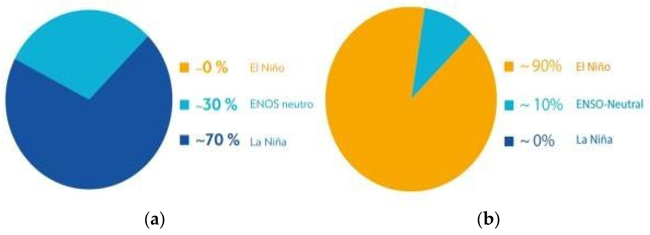
The effects of climate change have led to an increase in global precipitation, a phenomenon known as La Niña. This is particularly evident in Colombia, affecting the Andean, Pacific, and Caribbean regions. Figure 1a illustrates the occurrence of the third triple episode of La Niña (ENSO), which had a 70% probability of persisting until the end of March 2023. Forecasts indicated a 60% probability of an El Niño event from May through July 2023, with a 90% probability of continuing through October 2023, as shown in Figure 1b. This left a 10% probability of an ENSO neutral period and virtually no chance of another La Niña event by the end of October 2023.
Statistical and numerical applications are often not as effective in predicting precipitation accurately and timely, and although weather stations offer short-term predictions, forecasting long-term precipitation remains challenging [6,7]. Therefore, advancements are being made by integrating them with emerging technologies, like artificial intelligence. For instance, Ref. [8] implemented machine learning and observed that the forecast achieved better precipitation prediction compared to a deviation between 46% and 91% experienced in June 2019 in India. This progress involves leveraging historical data and using time series models to implement various machine learning (ML) and deep learning (DL) models, such as the OP-ELM algorithm, which demonstrated successful monthly rainfall predictions in China [9].
In the field of meteorological and hydrological prediction, the accuracy of long-term forecasts tends to decrease, especially when predicting higher intensities. However, new artificial intelligence techniques have significantly improved these predictions. Ref. [10] introduced a spatiotemporal feature fusion transformer that enhances the accuracy of precipitation nowcasting by effectively fusing spatial and temporal features. This model’s innovative approach to feature fusion and attention mechanisms is particularly relevant for developing methods aimed at monthly precipitation prediction.
Similarly, Ref. [11] presented a comprehensive framework for predicting the monthly runoff in the Xijiang River using gated recurrent units (GRUs), discrete wavelet transforms (DWTs), and variational modal decomposition (VMD). By leveraging antecedent monthly runoff, water levels, and precipitation data, this approach demonstrates substantial improvements in prediction accuracy, highlighting its applicability to monthly precipitation forecasting. Additionally, Ref. [12] used long short-term memory (LSTM) and neural hierarchical interpolation for time series forecasting (N-HiTS) to predict the standardized precipitation index (SPI) across various regions in Zacatecas, Mexico. Their combined modeling approach enhances the ability to predict SPI values, offering a valuable method for monthly precipitation prediction.
There are several ML versions, as demonstrated by [13] in their study predicting the normalized precipitation index using monthly data from 1949 to 2013 at four meteorological stations. Techniques included M5tree, extreme learning machine (ELM), and online sequential ELM (OSELM). The ELM model made the best predictions for months 3, 6, and 12, with the lowest root mean square error (RMSE) value, except for the predicted values for month 1, where the M5tree model obtained the best result.
DL is an emerging technique for dealing with complex systems, such as the prediction of meteorological variables. Therefore, Ref. [14] proposed a hybrid DL approach using a combination of a one-dimensional convolutional neural network (Conv1D) and a multilayer perceptron (MLP) (hereafter Conv1D-MLP) to predict precipitation applied to 12 different locations. The result was better and was compared with a support vector regression (SVM) machine learning approach. Similarly, using 92 meteorological stations in China, Ref. [15] combined the surface altitudes of the stations with the precipitation prediction, grouping by the k-means method, as implemented by [16], the stations surrounding the target and using a convolutional neural network (CNN), thus obtaining better results in the existing threat index and mean squared error (MSE).
Finding the best method for modeling the precipitation variable and the different parameters surrounding it is complicated. For this reason, Ref. [6] evaluated a model in Australia based on ML optimized with DL to predict daily rainfall and used GridSearchCV (version 1.5.1) to find the best parameters for the different models over a daily span of 10 years from 2007 to 2017 from 26 geographically diverse rain gauge locations. With the rise of ML and DL systems, remote sensing plays an important role since, according to [17], it allows the acquisition of terrestrial information from sensors installed on space platforms and the use of satellite images to perform multi-temporal analyses, understood as spatiotemporal changes [18,19]. In 2020, a CNN model was used with different architectures, such as GoogLeNet, AlexNet, and LeNet, among others [20], on 2D images as input precipitation data with three different heights: 100, 3000, and 5500 m above sea level. The output variable was an image that indicates to which class it belongs, converting the model to a binary class defined by a rainfall probability threshold between 0 and 100%. The main result was that CNNs can predict precipitation with lower computational capacity than traditional methods [21]. Two data sources were used for training and testing the CNN model. The first was the CEH, and the second was the Centre for Ecology and Hydrology Gridded Estimate of Areal Rainfall (GEAR), providing data on the monthly rainfall across Britain between 1890 and 2017. The results obtained from video-based rainfall prediction using different CNN architectures can provide valuable post-processing to traditional numerical weather prediction models.
The main concern for researchers studying precipitation in different geographical areas and climates worldwide has been the selection of suitable ML and DL methods. Hence, [22,23,24,25] have also presented various approaches for predicting precipitation. Table 1 evaluates techniques such as the Lagrangian convolutional neural network (L-CNN), the ELM model, the LSTM model, the multilayer perceptron (MLP) model, and the CNN model.

Formulation of the Research Question

What computational elements are necessary to implement a predictive model supported by deep learning that facilitates the spatiotemporal analysis of the monthly total precipitation in the department of Boyacá?

2. Materials and Methods

2.1. Dataset

The CHIRPS 2.0 dataset, though global, will be used to gather precipitation data specifically for the Boyacá Department, Colombia. This dataset will be collected monthly and used exclusively to predict precipitation values in millimeters (mm). Thus, the primary focus of the project is the research and development of deep learning models, without an immediate practical application.
Climate Hazards Group InfraRed Precipitation with Station data (CHIRPS), which integrates infrared precipitation data with station data, was used for this project. This dataset was developed by the Climate Hazards Group at the University of California, Santa Barbara [26]. The CHIRPS dataset provides more than 35 years of comprehensive and accurate precipitation information worldwide. For this study, infrared precipitation data were extracted from January 1981 to August 2023 for the Boyacá department. The data were acquired at a resolution of 0.05°, with each degree corresponding to 111.1 km, resulting in a data acquisition resolution of approximately 5.5 km.
Using tools such as Python 3.12.5 [27], Google Collaboratory [28], TensorFlow [29], Keras 3.0 [30], and Matplotlib 3.9.0 [31], among others, the project was developed as follows: The results obtained will serve as a foundation and reference for the macro project “Application of Machine Learning in the Spatiotemporal Prediction of Total Monthly Precipitation in the Boyacá Department”, identified by the code SGI 3535 and developed by the GALASH research group at the Pedagogical and Technological University of Colombia.
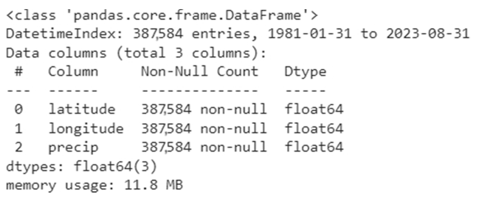
The downloaded dataset was processed in netcdf (.nc) format, containing monthly precipitation records worldwide, spanning 43 years and 8 months, with 3 variables, longitude, latitude, and precipitation in (mm), along with a time variable indicating the date of measurement in datetime [ns] format. This format enables manipulation of the dates and times at which the data were collected, as illustrated in Figure 2. It provides the dataset with the spatiotemporal focus required for predicting precipitation, comprising a total of 387,584 observations.

2.2. Methodology

Case Study

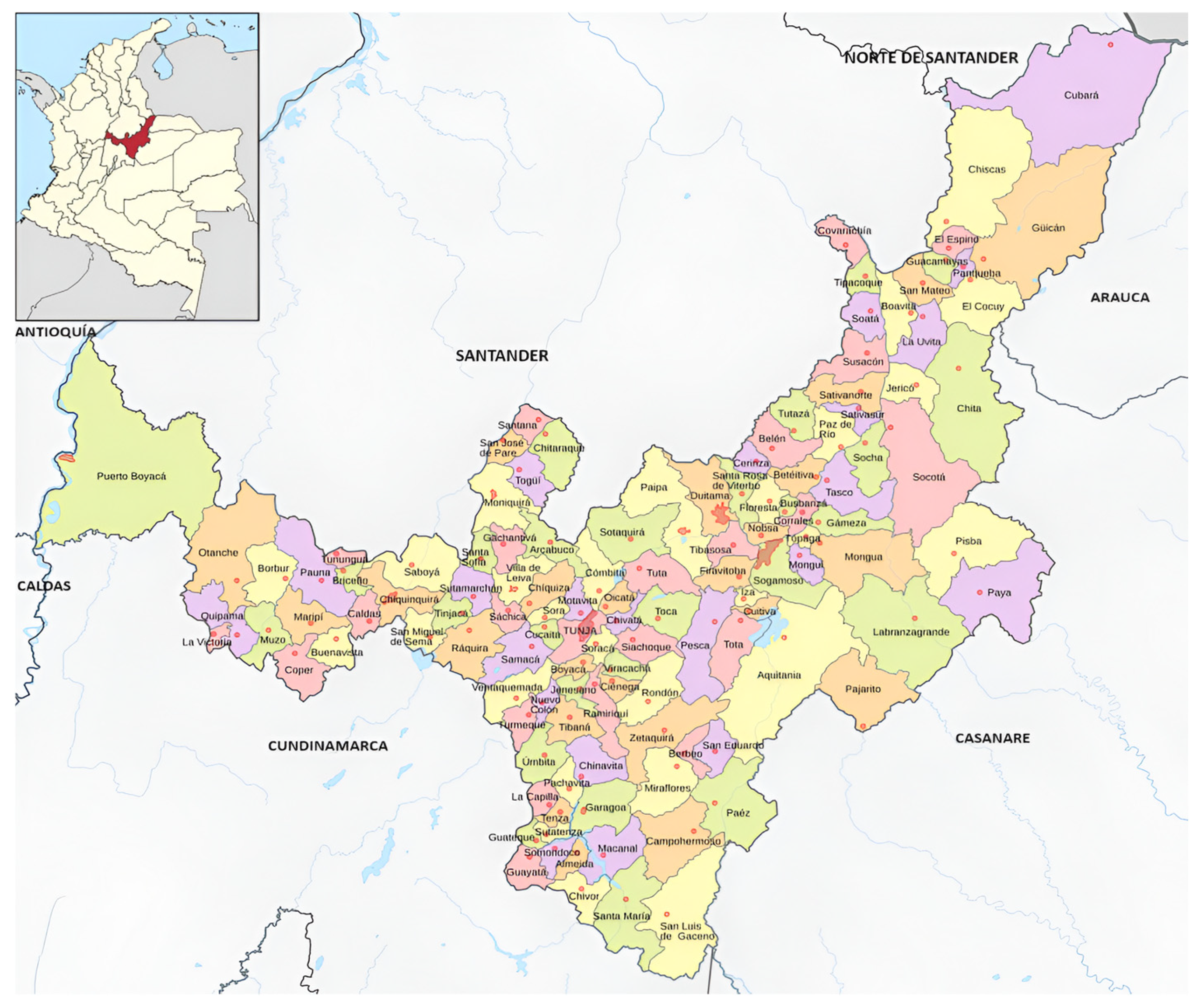
This project is currently underway in the Boyacá Department, situated in the Andean region of central Colombia. Boyacá is well known for its agricultural activity, emphasizing the importance of precipitation forecasting in decision making related to agriculture and water resource management in the region. Figure 3 clearly illustrates the geographic location of Boyacá.
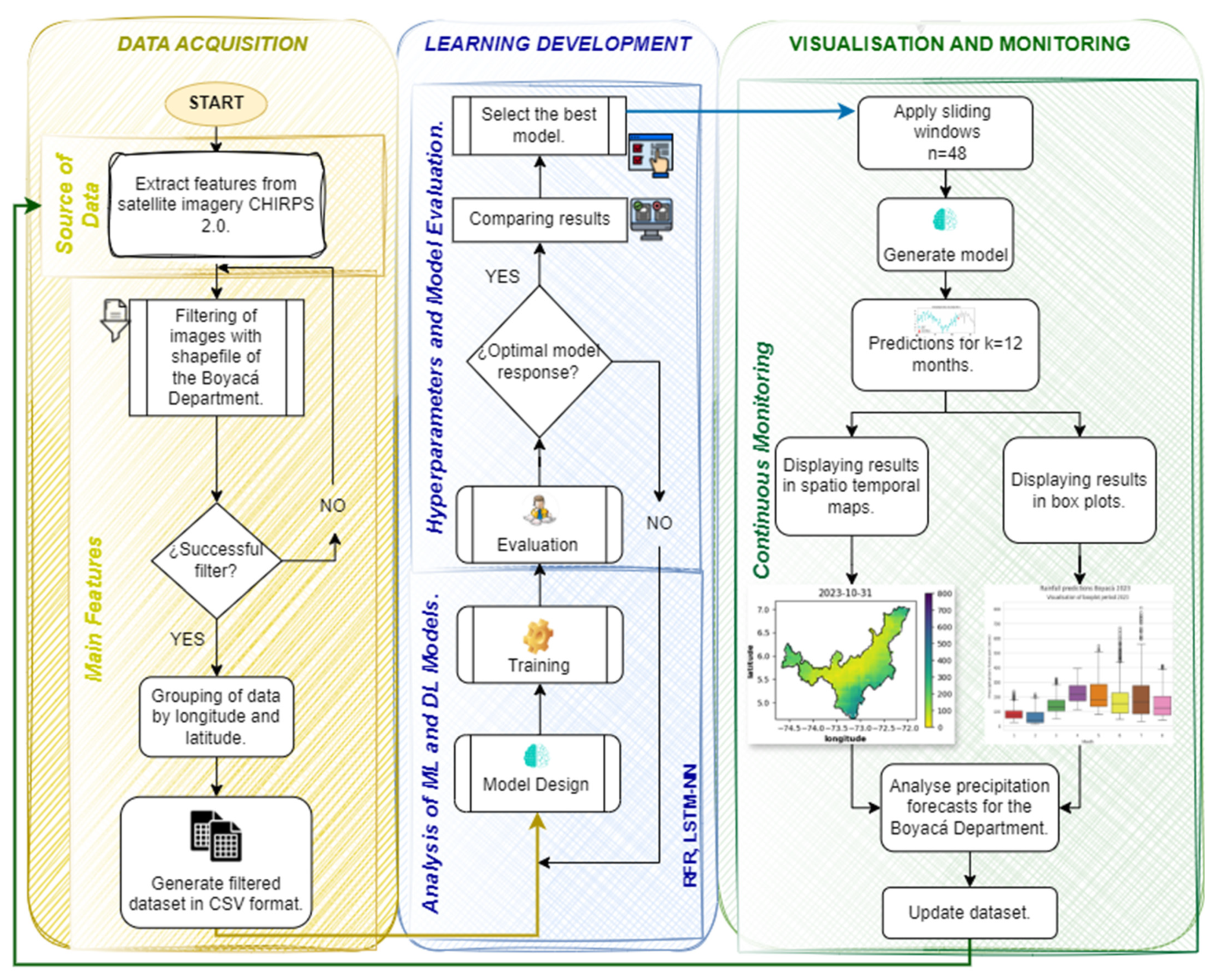
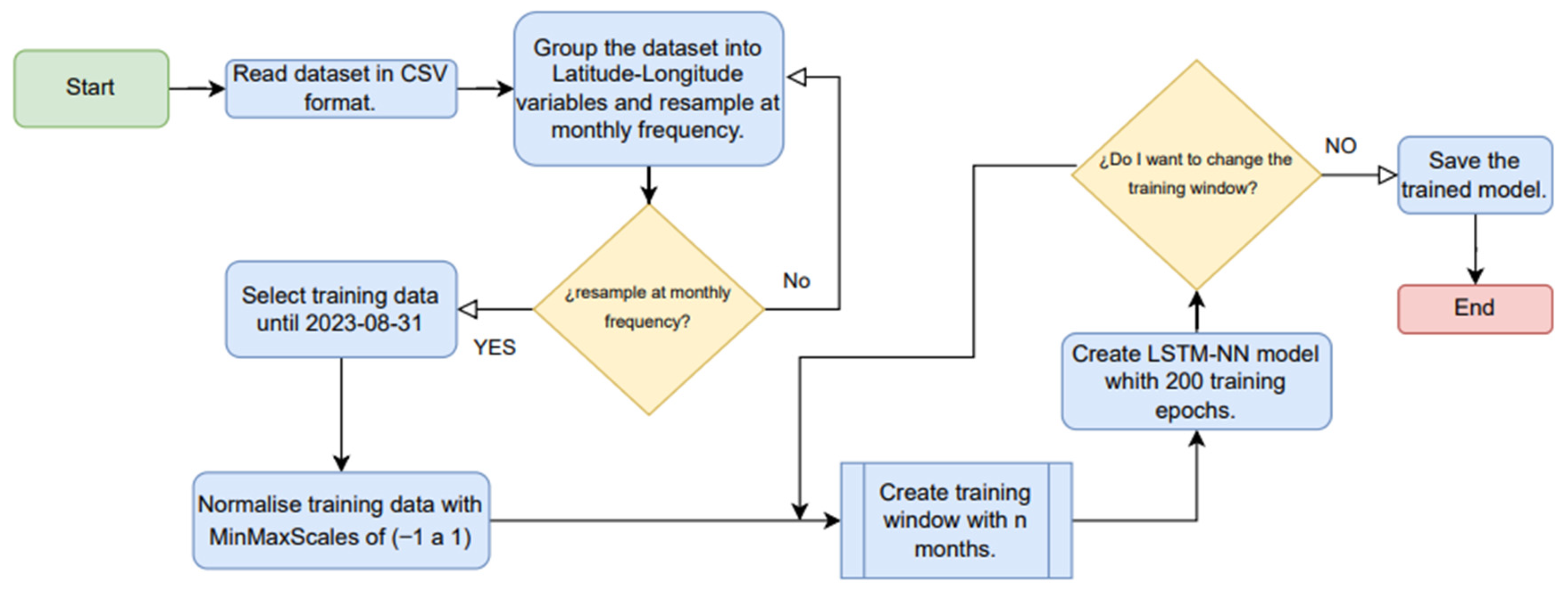
To implement methodologies for developing predictive models of total monthly precipitation using satellite images, we adapted the ML-OPS model methodology, as illustrated in Figure 4. This approach enhances the quality and coherence of the project solution by integrating artificial intelligence, ensuring rigorous quality control in model development and implementation. The process of implementing the models to be evaluated comprised the following stages:
  • Step 1: Data Acquisition (ML)
During the background review, a dataset (CHIRPS) containing monthly precipitation information in millimeters worldwide was identified that has a size of 6.64 GB with a spatial resolution of 0.05° (5.5 k), which includes 3 floating-type data, longitude (unit: degrees north), latitude (unit: degrees east), and precipitation (unit: mm), and a time-type data (unit: yyyy/mm/dd). On this dataset, geographic filtering was performed to obtain only the coordinates of the department of Boyacá.
2.
Stage 2: Developmental Learning (DEV)
According to the literature, the algorithms that gave the best response in predictions were used; therefore, an LSTM-NN deep learning model was analyzed and compared with ARIMA time series and regressive random forest (RF-regressive) machine learning algorithms, where a training set with 387,584 observations was defined. The multivariate dataset was obtained as input using scaled data with the Sklearn pre-processing class.
MinMaxScaler was used to normalize the data so that a range from −1 to 1 was established, obtaining at the output a monthly precipitation value with scaled data in each of the geographic coordinates of the existing data, in addition to improving performance by tuning the hyperparameters according to the model evaluated; for example, in the ARIMA and RF-regression models, stationarity characteristics were evaluated.
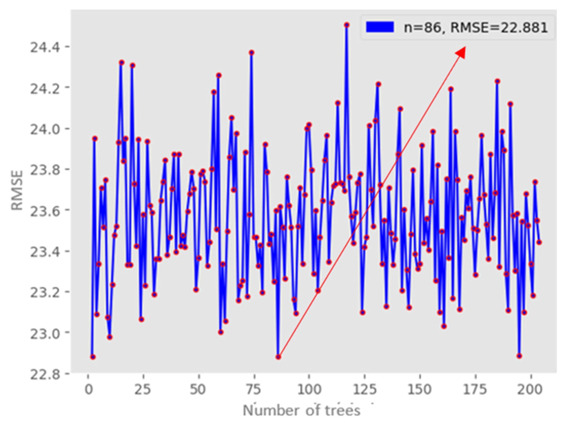
A Dickey–Fuller (DF) test was performed on the time series to check whether the data exhibit a unit root autoregressive process [32], which indicates whether the model is stationary. Once the time series rejects the null hypothesis and the data are stationary, it confirms stationarity. In addition, the number of trees in the random forest was determined by evaluating the lowest RMSE value between 0 and 200 trees.
The models were evaluated using RMSE, MAE, MAPE, and R2 metrics (see Section 2.4), and which model achieved the best performance on the evaluation set and minimized the error was determined. The selected model was then used to make predictions for 16 months, comprising the remaining 4 months of the year 2023 (September to December) and the 12 months of the year 2024.
3.
Stage 3: Monitoring and Supervision (OPS)
Various tests were conducted on the models until hyperparameters were identified, which provided satisfactory results on both the training dataset and various test datasets. This was done to maximize the model’s accuracy on the test set and continuously reduce residual errors in future predictions.

2.3. Evaluation Models

2.3.1. Autoregressive Integrated Moving Average (ARIMA) Model

It is a model used to predict future trends in time series and regression data. Introduced by Box and Jenkins in the 1970s, the ARIMA model forecasts the future value of a variable as a linear combination of past values and past errors [33]. It is expressed as follows: the autoregressive model order (p), the differencing order (d), and the moving average model order (q) [34,35].
The ARIMA (p, d, q) model for time series γ t {t = 1, 2, 3, n} is as follows:
γ t = θ 0 + φ 1 γ t - 1 + φ 2 γ t - 2 + + φ p γ t - p + ε t θ 1 ε t - 1 θ 2 ε t - 2 θ q ε t - q
where γ t is the true value; t is the random error in time; φ i and θ j are the coefficients; and p, d, and q are integers, which are usually autoregressive, differenced, and moving average polynomials, respectively.

2.3.2. Random Forest Regression (RF-R) Model

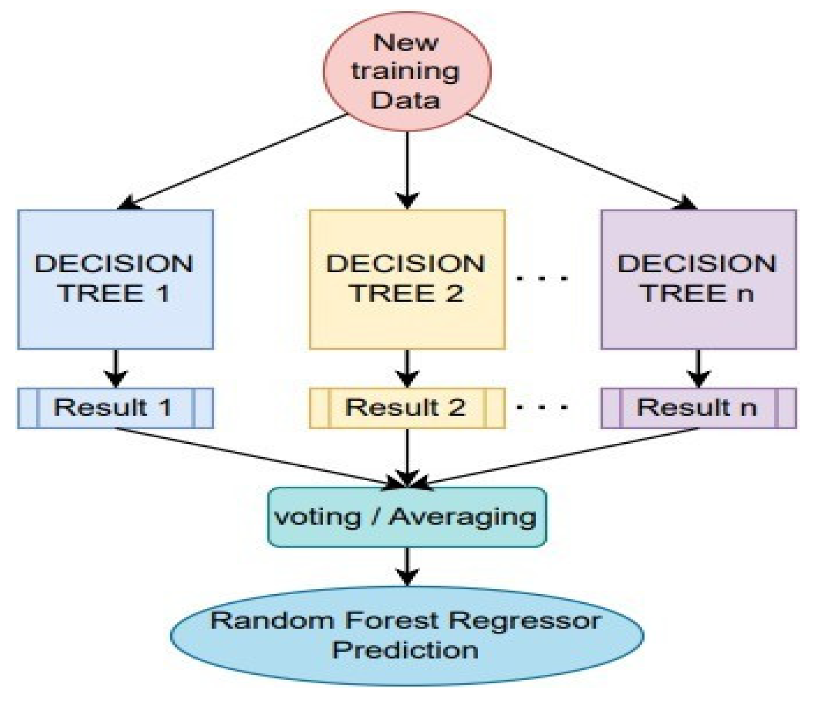
It is a classifier structured as a tree. Given the set of classifiers {h (Xξk), k = 1}, where each (ξk) is independent, this model relies on a combination of tree predictors. These predictors depend on the values of an independently sampled random vector. Each tree makes a decision and outputs a unit vote for the class [36]. Finally, the results of the random subsets created are averaged, and a prediction value is obtained, as shown in Figure 5.

2.3.3. Long Short-Time Memory (LSTM) Neural Network Model

The LSTM model was first proposed by Hochreiter and Schmidhuber in 1997 and has since become particularly renowned as one of the best time series prediction methods [37] In its design, the LSTM model comprises gating units and memory cells of a neural network. These memory cells store recent data, and when new information arrives, it is controlled by the combination of the cell state, which is then updated. Each time new information is received by the memory cell, the output is processed with this new information. The LSTM network is particularly effective for long-term problems as it can retain information over extended periods. Its structure includes two tanh layers, as depicted in Figure 6.
The LSTM model can selectively exclude data from the cell through its gate structures, as these gates control whether data enters the cell. The gates are governed by the sigmoid function, which generates values ranging from 0 to 1. A value of 0 indicates that “nothing happens”, while a value of 1 signifies that “everything happens” [39].
The gating mechanism is implemented using the sigmoid function and the dot product operation (refer to Equation (2)). There are three types of gates used in LSTM networks, the update gate, the forget gate, and the output gate, as identified in Equations (3)–(5) [37,38]. These gates facilitate the flow of information from one cell to another. Consequently, the LSTM cell produces two outputs, the activation and the candidate value, as illustrated in Equation (6).
g   x = σ   W   x + b
where σ is the sigmoid function, and the expression is σ   x = 1 + 1 exp exp - x .
Upgrade   gate :   Γ u = σ ( W u [ h < t - 1 > , x t ] + b u )  
Door   of   oblivion :   Γ f =   σ ( W f [ h < t - 1 > , x t ] + b f )  
Exit   door :   Γ o = σ ( W o [ h < t 1 > , x t ] + b o )  
Outputs :   c <   t   >   = Γ u × c N <   t   > + Γ f × c <   t - 1   > a <   t   >   = Γ o × c <   t   >

2.4. Evaluation Metrics

2.4.1. Root Mean Square Error (RMSE)

It is the error between the distance of the residual values in the prediction and their actual values.

2.4.2. Mean Absolute Error (MAE)

It is an average error of absolute differences between the prediction and its actual value, being less sensitive to outliers.

2.4.3. Mean Absolute Percentage Error (MAPE)

It is a percentage error between the predicted value and the actual values and gives a scale-independent view of the error.

2.4.4. R Square (R2)

It is the percentage of accuracy between the predicted measurement and the actual measurement.

3. Results

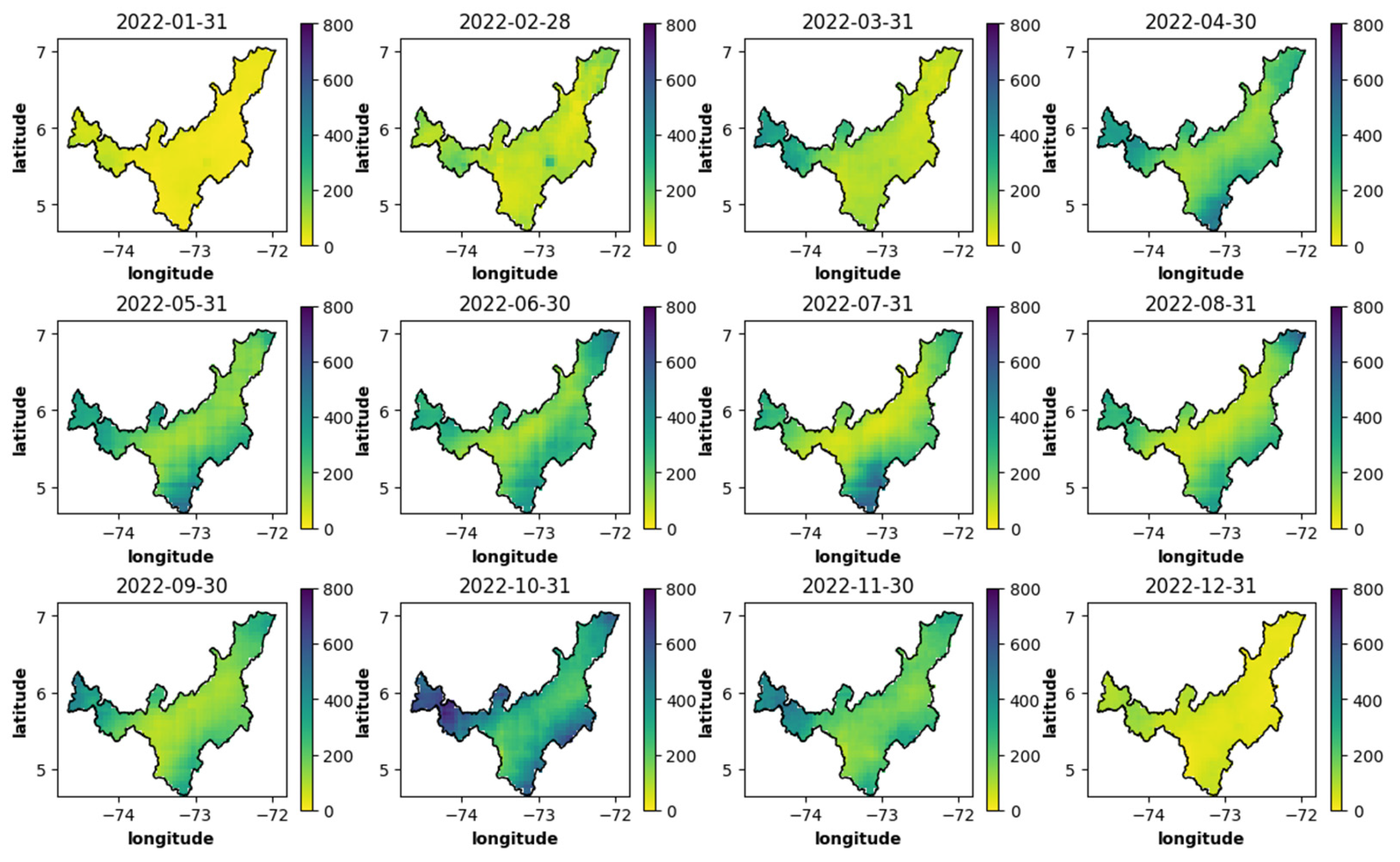
In surveying and geography, spatial analysis is a widely used technique for collecting information from specific sampling points. The coordinates were used to filter the CHIRPS precipitation data for Boyacá, Colombia, using the department’s polygon. Subsequently, the dataset was organized to visualize the spatiotemporal dimension for climate analysis through time, as depicted in Figure 7, illustrating the spatiotemporal precipitation of Boyacá in the year 2022.
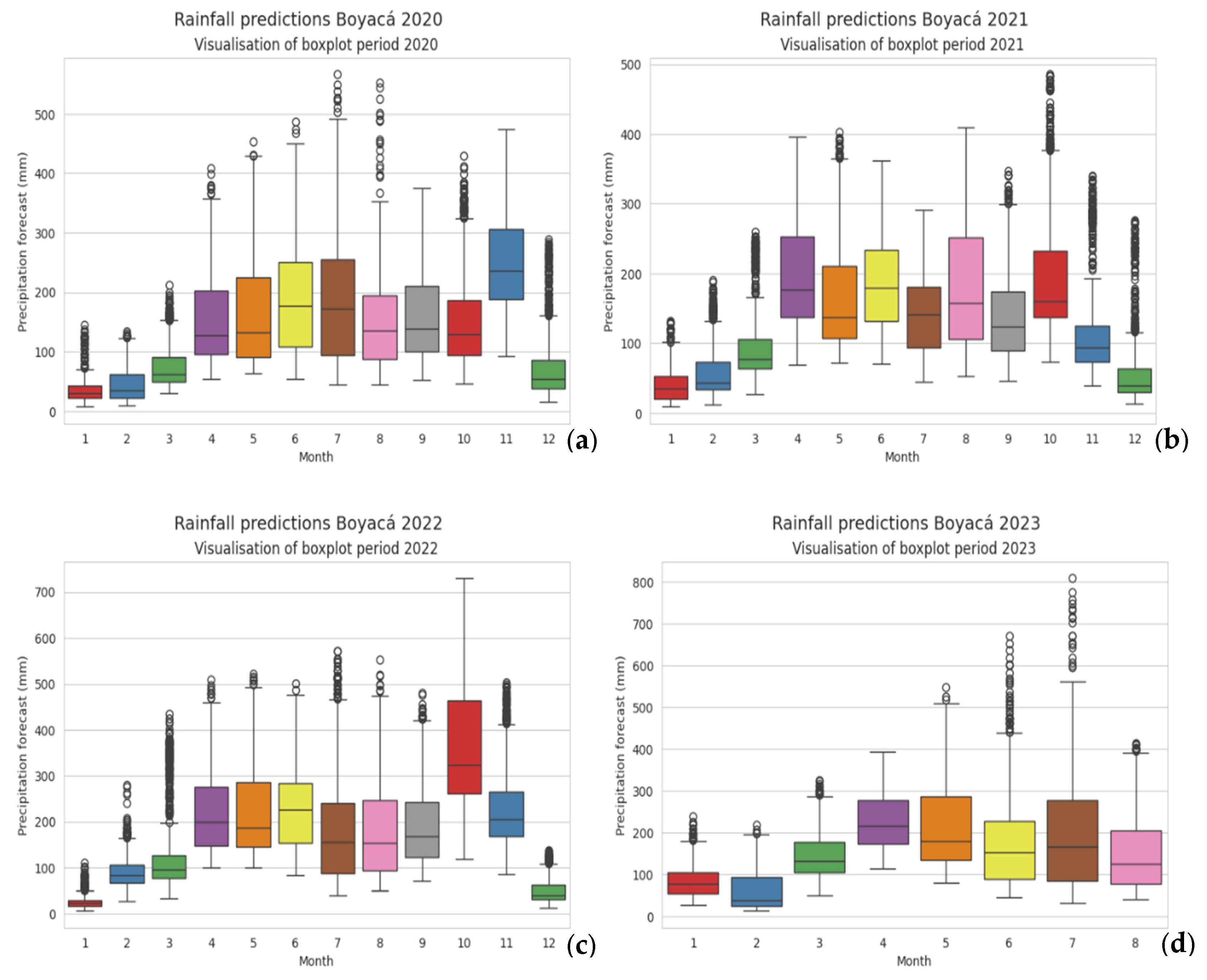
An analysis of historical precipitation values from 2020 to 2023 was conducted using box-and-whisker plots, presenting quantitative distribution through quartiles, as shown in Figure 8a–d. Based on the acquired and organized stationary precipitation data, along with statistical analysis, patterns and trends in and relationships between the dataset’s characteristics can be identified. According to [40], the box-and-whisker plot facilitates the establishment of relationships between samples and the identification of outliers.
Examining the distribution of precipitation in Boyacá, it was observed that in the year 2020, the maximum precipitation occurred in July, reaching approximately 500 mm. Additionally, some outlier precipitation points exceeded this value, suggesting the presence of a geographical area with significant monthly precipitation, such as a moor or an anomaly within the dataset for that year. Upon investigating these outliers, it was found that the coordinates corresponding to latitude 7.024998 and longitude −72.125008, located in the municipality of Cubará, Boyacá (see Figure 3), in the northeast of the region, experience high rainfall. This indicates that it is not an outlier but rather a location with a high probability of significant precipitation.
In 2021, the dry-season months (January to March) did not exceed an average of 100 mm of monthly rainfall, although March saw rainfall exceeding 200 mm. The rainy season, with precipitation averaging between 150 and 200 mm, persisted from April to October, with October being the wettest month, recording rainfall over 400 mm.
In 2022, the effects of climate change were evident, with maximum precipitation values from May to November exceeding 400 mm and in some months reaching approximately 500 mm. In October, some data showed values exceeding 700 mm, without any outliers, representing a significant increase compared to previous years, when precipitation values did not exceed 400–450 mm per month.
For 2023, rainfall ranged between 150 mm and a maximum of 300 mm until March. From April to October, the El Niño phenomenon was expected, resulting in decreased departmental precipitation, averaging 200 mm per month. This analysis indicates that the dry season occurs between January and March, with December having moderate rainfall. Months with average rainfall are between April and August, while the highest rainfall occurs from September to November, with October experiencing the highest rainfall in the two years 2021 and 2022.

3.1. Development of Predictive Models

The dataset for each of the models was divided into 70% for training and 30% for testing. The results of the ARIMA, RFR, and LSTM models are presented next.

3.1.1. ARIMA Model Design

A Dickey–Fuller (DF) test was conducted on the time series to determine whether the data adhere to a unit root autoregressive process [32], indicating the stationarity of the model. Once the time series rejected the null hypothesis and the data were stationary, precipitation was selected as the target variable. The best model for the training set was identified as the autoregressive and differenced ARIMA model (4,1,0) (2,1,0) (12), lacking moving average characteristics (i.e., a stationary model), with four lag observations in the autoregressive model and one degree of differencing.
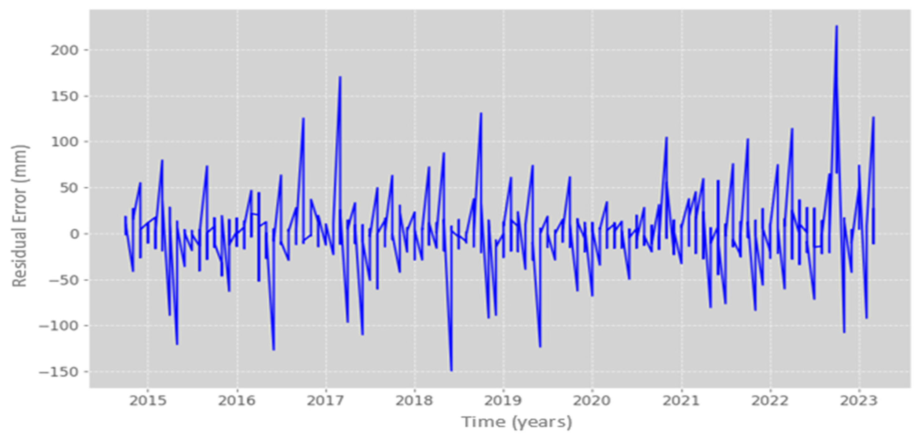
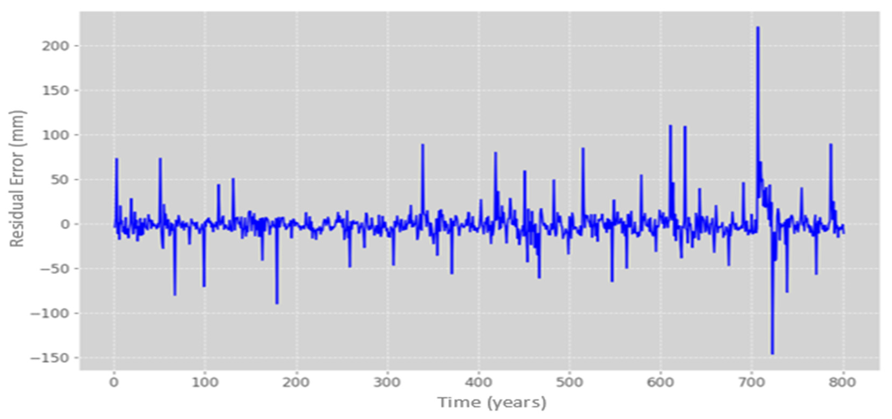
Finally, the model’s predictions were evaluated, achieving an 81% similarity to the observed precipitation in both training and test datasets, with residual errors averaging 27.98 mm compared to the actual measurements. The error trend across most data points exhibited a mean of zero and a uniform variance, although there were instances where the residual error exceeded 200 mm, as illustrated in Figure 9.

3.1.2. Random Forest Regression Design

In this model, seasonal variables of year and month were included in each observation of the input dataset. Additionally, one year’s worth of data were included for each observation. Consequently, a dataset with 17 variables (latitude, longitude, precipitation, year, month, L1, …, L12) was obtained, where precipitation served as the target variable and the other variables acted as labels for prediction.
A random forest regression model with 83 decision trees was created. This specific number of trees was chosen as it produced the lowest RMSE value among the 0 to 205 trees evaluated, as shown in Figure 10.
The study achieved an 87% similarity between the model’s precipitation predictions and the observations from the training and test datasets. When plotting the model’s response against the test dataset, it was observed that the predictions closely matched the actual behavior in most instances. However, there were a few outliers where the predictions deviated by approximately 12 mm from the actual values, resulting in an overall error of 23.21 mm, as illustrated in Figure 11.

3.1.3. LSTM-NN Model Design

Several training runs were conducted for the LSTM model, exploring different hyperparameter values. The best model achieved included a sequential class instance with 128 memory units in the hidden layers, using a linear activation function and a mean squared error (MSE) loss function, with a learning rate set to RMSprop.
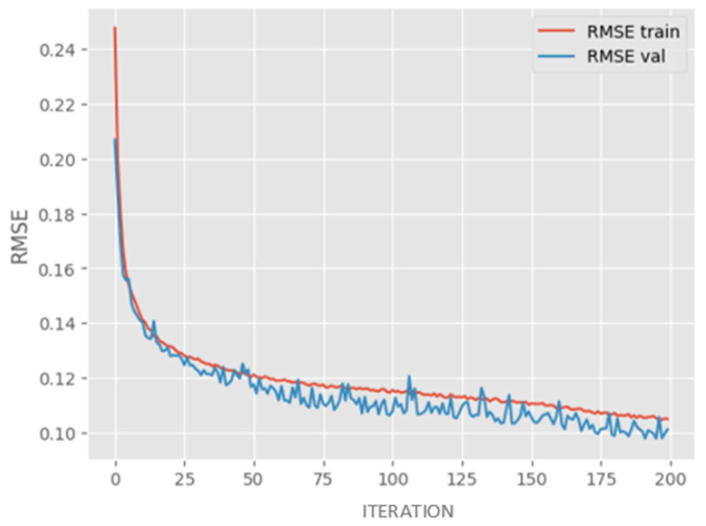
Furthermore, validation for overfitting was performed on the training and test datasets, as illustrated in Figure 12. Upon converting the predictions to full scale, the LSTM model demonstrated 92% effectiveness in reproducing the precipitation values of the dataset. This resulted in a 16-percentage point reduction in the residual error compared to the random forest regression (RF-R) model. Additionally, the LSTM model showed a decrease in the number of significant errors, with only a few iterations exhibiting values above 100 mm and one instance of approximately 200 mm, as shown in Figure 13.
In the evaluation metrics, three models were compared: the ARIMA model, the LSTM-NN model, and the random forest regressor. The ARIMA model demonstrated efficiency but exhibited 10% lower reliability in predictions compared to the LSTM-NN model, as detailed in Table 2. Additionally, the root mean square error (RMSE) of the ARIMA model was more than 10% higher than that of the other two evaluated models. Consequently, the LSTM-NN emerged as the best model for reproducing observations from the dataset, with an error rate of 0.8% and a superior RMSE metric compared to the second-best model, the random forest regressor. The monthly precipitation errors, whether above or below the actual measurements, were approximately 10 mm.
Based on the evaluated results, the LSTM-NN model is the most effective in reproducing precipitation observations from the training and test datasets. Consequently, this model was implemented to predict precipitation over the next 48 months, starting from the last month, which was August 2023.

3.2. LSTM-NN Model Implementation

The implementation was based on the LSTM-NN model capturing spatiotemporal patterns of monthly precipitation data for the Boyacá department with the following architecture:
  • LSTM layer with 128 hidden units
The decision to use an LSTM layer with 128 units was based on its ability to yield the best results, leading to an improvement in the RMSE value. It is worth noting that increasing the number of hidden layers in the model tends to result in more accurate predictions. However, it is important to exercise caution, as the number of layers determines the amount of information the layer can learn. Therefore, there is a risk of overfitting of the training and test data if this number is increased excessively.
  • Rectified linear unit (ReLu) activation function
This function was used so that training would be fast and there would be no saturation, as occurs with functions such as sigmoidal and hyperbolic tangent, and it is computationally simpler to implement.
  • Dense output layer
The objective of prediction was to perform a regression; therefore, a dense layer with a unit was used, which was the prediction on the precipitation variable.
  • Adam optimizer (adaptive moment estimation)
It is a method to accelerate the training of neural networks and achieve a near-linear acceleration rate with the increase in computational nodes [41]. It was selected to speed up the LSTM model, as it can adapt to learning each parameter individually and can lead to a lower prediction error compared to other algorithms.
  • Mean squared error (MSE) loss function
The MSE loss function gives more importance to large errors or outliers by providing a quadratic loss function as it squares and subsequently averages the values. This method is used in many identifications, prediction, and optimal filtering applications [42].
  • Sliding windows method
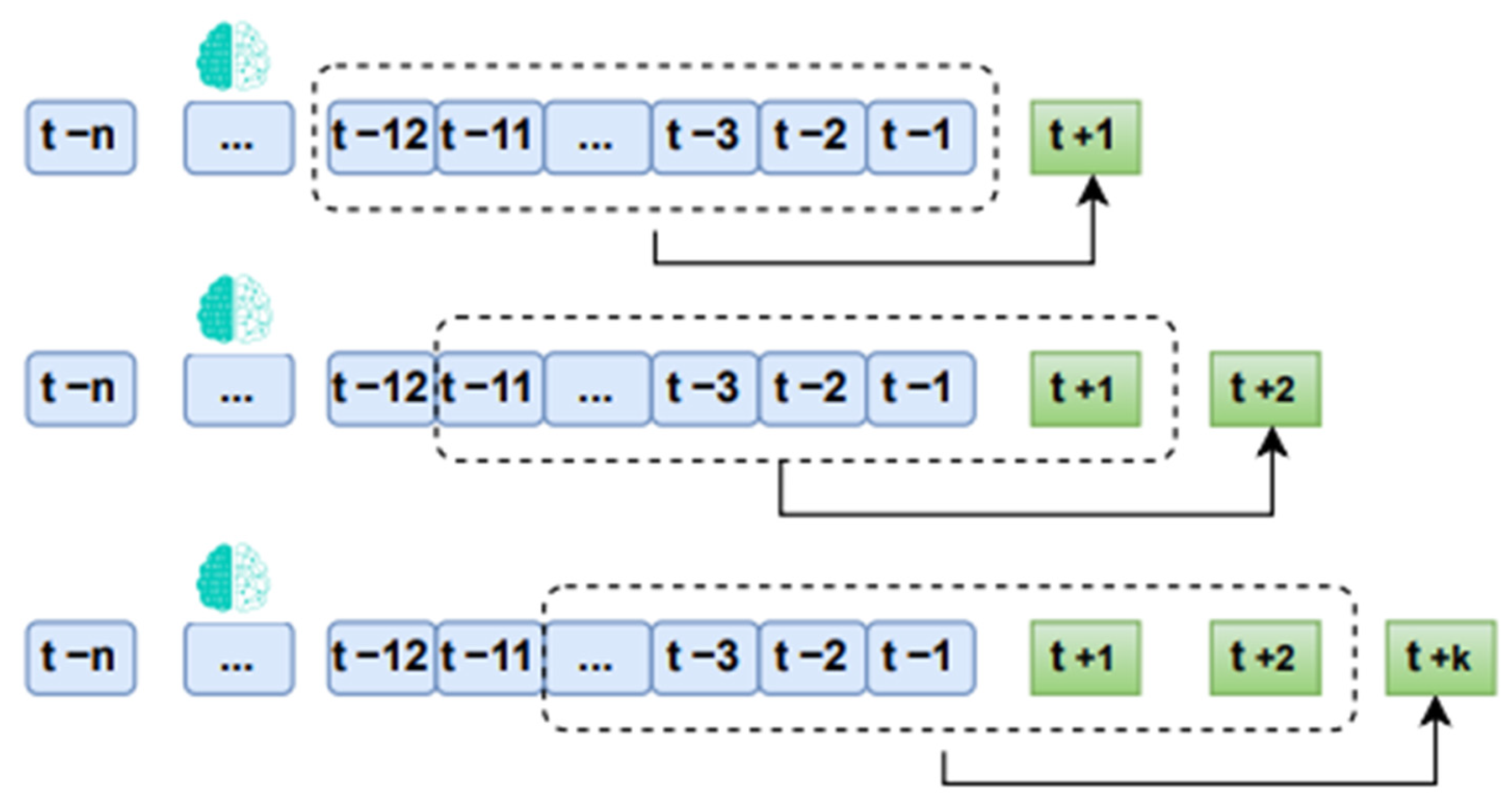
A sliding windows approach was used, wherein several previous months (t + n) were used to make predictions. This concept, known as sliding windows, was used to repair the input data for the training model. Subsequently, an algorithm was developed to construct a dataset comprising n number of previous months, with the output obtained for k following months using the architecture of the LSTM model mentioned before (refer to Figure 14).
The sliding windows model significantly enhances the accuracy of short-term monthly precipitation prediction when using deep long short-term memory (LSTM) recurrent neural networks, which segment the input data [43]. In this project, the 48-month window size was reconsidered to account for the El Niño and La Niña phenomena present in the region. Therefore, a 48-month window was established to predict at (t + 16), the first prediction commencing in September 2023 for each dataset and concluding in December 2024. The process detailing the handling of training data windows is illustrated in Figure 15.
The dataset contained a total of 757 geographical points of latitude and longitude of the Boyacá Department. Once validated, the model was trained and run on Google Collaboratory, which has the advantage of running Python 3 code in a runtime environment that uses T4 GPU hardware acceleration and high RAM capacity. A CSV-type dataset was generated with the columns latitude, longitude, time, and precipitation prediction in millimeters (mm), which allowed the generation of heat maps and box-and-whisker plots for each month.

LSTM-NN Forecast with a 48-Month Window

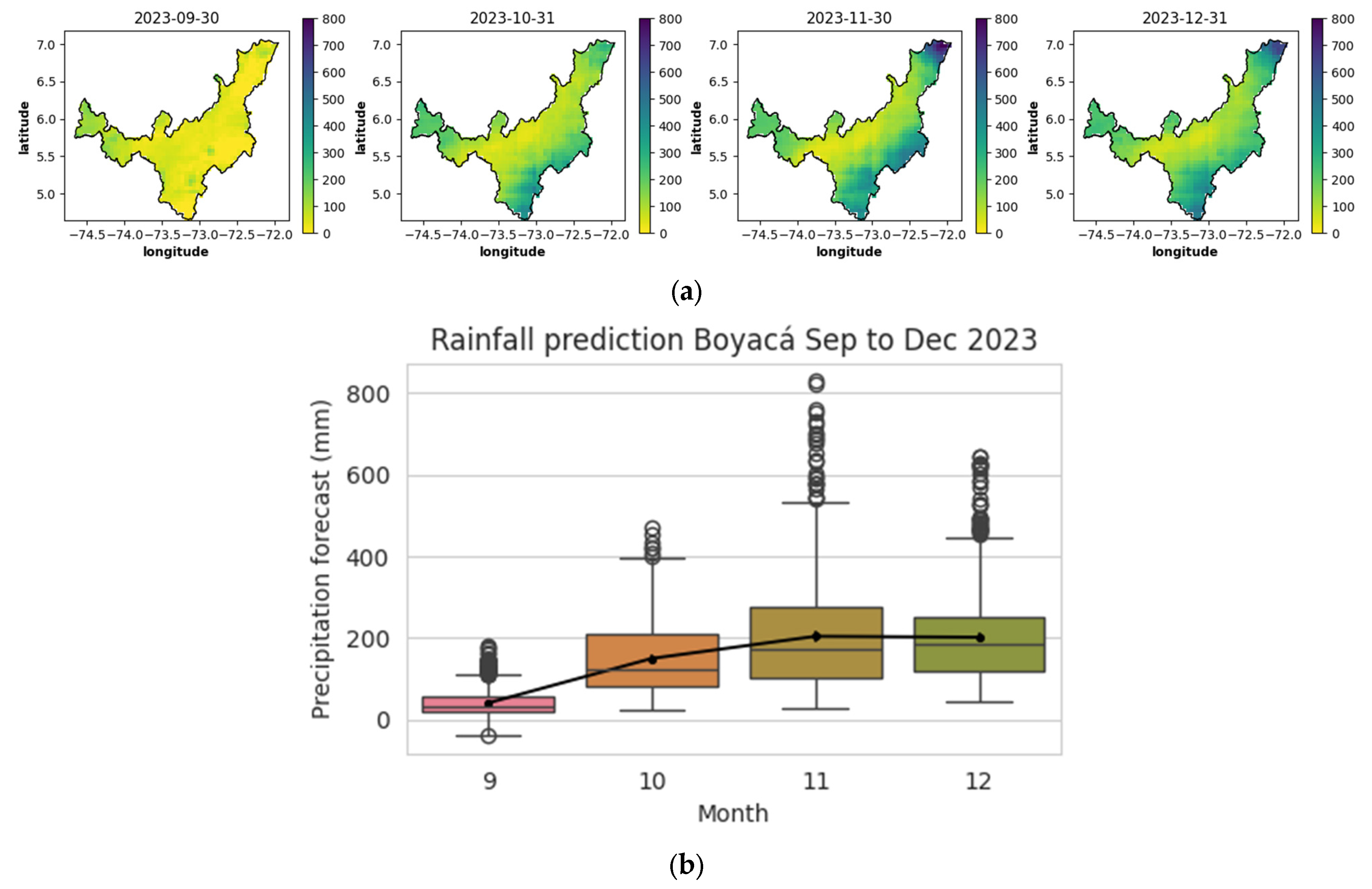
The training of this model was conducted in Google Collaboratory, following the specified configurations and using 200 epochs, lasting approximately 2 h. Figure 16a illustrates the spatiotemporal precipitation data, and Figure 16b represents the predicted values in box-and-whisker plots obtained for the remaining 4 months of the year 2023, starting in September.
The data indicated that precipitation levels for September were relatively low, as evidenced by the median, which fell below the 50th percentile of the data distribution. Forecasted precipitation values were expected to remain low, not exceeding 150 mm. However, the mean suggested a right-skewed distribution, with higher precipitation values leading to potential increases up to 200 mm per month across the entire Boyacá Department. This value was close to the average precipitation for this month.
For October, an increase in precipitation was expected, indicating a wetter month compared to September. The mean was slightly higher than the median, suggesting once again a right-skewed distribution, with some extreme values influencing the mean. The box-and-whisker plots (see Figure 16b) showed that from October to December, there were outliers exceeding 400 mm, and in October, these values ranged from 600 to 800 mm. However, when these results were compared with the spatiotemporal diagrams in Figure 16a, it became evident that these were not outliers but rather represent potential precipitation data in municipalities located on the borders and boundaries with the Departments of Antioquia, Caldas, Cundinamarca, and Norte de Santander (see Figure 3).
Regarding November, the mean continued to rise, while in December, it slightly decreased, indicating persistently high precipitation levels in the municipalities bordering the department and a trend of moderate precipitation, around 200 mm, in the central region.
A spatiotemporal prediction of precipitation for 2024 was conducted, revealing, as shown in Figure 17a, that during the first quarter, precipitation was expected to range from low to moderate, between 100 and 300 mm, with a slight decreasing trend. In Figure 17b, it is observed that during the first quarter, the median and mean precipitation values remained relatively close to each other, suggesting a symmetrical distribution of the data with few outliers. March was projected to end with the lowest precipitation levels, below 200 mm, indicating a particularly dry start to the second quarter.
As observed in the first quarter, March exhibited a decreasing trend in precipitation values. This trend continued into the second quarter, with a notable decline, particularly in May and June, where the average precipitation was approximately 70 mm, reaching maximum values of up to 200 mm across the three months. In the third quarter, a shift from the dry conditions of the previous quarter was expected, with July experiencing low-to-moderate rainfall, averaging around 230 mm, similar to the levels seen at the beginning of the year. Higher precipitation values were anticipated near the department’s borders, with some outliers exceeding 400 mm.
August was projected to be the wettest month, with intense rainfall ranging from 400 to 500 mm, and certain municipalities within the department could record peaks of up to 700 mm. The mean precipitation surpassed the median, indicating a potential presence of extreme high values.
For the final quarter, precipitation values are expected to remain relatively constant, with the mean and median being close, suggesting a uniform distribution of rainfall of around 200 mm per month. In the northeastern and southeastern parts of the department, precipitation levels may fluctuate between 350 and 400 mm per month.

4. Discussion

When compared with traditional models, such as ARIMA and random forest regression, the LSTM model demonstrates superior performance in accurately predicting precipitation, particularly in capturing the nuances of outlier data, which in the Boyacá region are not entirely outliers but rather data from municipalities or areas with high precipitation, mostly located at the department’s borders or extremities. The effectiveness of the LSTM model can be attributed to its ability to retain and learn from sequential dependencies within time series data, enabling it to better model the complex and nonlinear patterns inherent in precipitation datasets.
The results from the LSTM model indicated significant seasonal variations in precipitation, with a notable dry period forecasted for the second quarter of 2024, particularly in May and June, followed by a transition to wetter conditions in the third quarter. The model’s ability to predict such transitions is crucial for water resource management, agricultural planning, and disaster mitigation strategies, especially in regions with variable climatic conditions, like Boyacá, where 24% of Colombia’s páramo areas are located. The accuracy of the LSTM model in predicting extreme precipitation events, such as those expected in August, with up to 700 mm of precipitation, will be highly beneficial for early-warning systems in flood risk management.
Despite the strengths of the LSTM model, our study reveals limitations in current prediction approaches, particularly given the diverse topography of Boyacá, which includes mountainous areas, valleys, and plains that significantly influence precipitation patterns. The model’s performance could be enhanced by incorporating additional topographic features, as demonstrated in the study by [11] on the monthly runoff prediction for the Xijiang River. By using a combination of GRU, DWT, and VMD, their research highlights substantial improvements in accuracy by leveraging historical data on runoff, water levels, and precipitation.
Integrating additional topographic variables during training, such as altitude, water levels, and runoff, could improve the spatial resolution of our model and reduce residual errors. This would not only enhance the prediction of extreme precipitation events but also better capture microclimatic variations in a region as diverse as Boyacá.
The comparison with ARIMA and random forest regression models underscores the robustness of the LSTM model in handling time series data with long-term complexities. Although ARIMA models are traditionally preferred for their simplicity and interpretability in forecasting linear time series, their limitations become evident when faced with nonlinear climatic data. Random forest regression offers strong predictive performance with the advantage of feature importance evaluation; however, it struggles with the temporal dependencies that LSTM models manage effectively. This confirms the use of neural networks, as also demonstrated by a study conducted in Zacatecas, Mexico [12], where a combined modeling approach for predicting the Standardized Precipitation Index (SPI) enhanced the ability to predict SPI values, providing a valuable method for monthly precipitation forecasting. This further validates the efficacy of advanced neural network models in handling the long-term complexities of climatic data. The strength of this method lies in the hierarchical interpolation of time series, enabling the effective capture of temporal patterns across multiple scales.
The application of the LSTM model in this study has broad implications beyond the department of Boyacá. The methodology demonstrated here can be adapted for precipitation prediction in different regions, provided that local geographic and climatic conditions are considered in the model-training process. This adaptability makes the LSTM model a powerful tool for regional climate modeling and water resource management, as it integrates spatiotemporal features. This contrasts with the spatiotemporal feature fusion transformer implemented by [10], which enhances the prediction of complex precipitation patterns. This reaffirms that the use of spatiotemporal variables can potentially reduce residual errors and improve the accuracy of long-term forecasts.
Future work should explore the potential of combining LSTM models with other advanced machine learning techniques, such as hybrid models, to further improve prediction accuracy and reduce residual errors. Additionally, expanding the model to include dynamic climate variables, such as the sea surface temperature anomalies associated with El Niño and La Niña phenomena, could enhance long-term forecasting capabilities. As climate change continues to impact precipitation patterns globally, these advancements in predictive modeling are essential for proactive adaptation and mitigation strategies.

5. Conclusions

The implementation of the LSTM-NN model, leveraging the sliding windows method, achieved accurate predictions of precipitation patterns in Boyacá for the 16 months spanning September 2023 to December 2024. The results demonstrated the model’s superiority in capturing the subtleties of outlier data and seasonal variations, attributed to its ability to learn from sequential dependencies in time series data. This capability enables precise long-term predictions, crucial for informing water resource management, agricultural planning, and disaster mitigation strategies in Boyacá, Colombia.
The findings also underscore the importance of considering local geographic and climatic conditions during model training, as well as the potential for enhancement through the integration of topographic features and dynamic climatic variables.
Future research should focus on combining models to mitigate residual errors, incorporating altitude and other pertinent variables, and expanding the model to encompass dynamic climate variables. By building upon these results, we can enhance predictive modeling capabilities, enabling proactive adaptation and mitigation strategies to address climate-related challenges in Boyacá and other departments of Colombia.
Author Contributions

Conceptualization, J.S.N.M. and M.J.S.B.; methodology, J.S.N.M.; software, J.S.N.M.; validation, J.S.N.M., M.J.S.B. and J.A.R.S.; formal analysis, J.S.N.M.; investigation, J.S.N.M.; resources, J.S.N.M., M.J.S.B. and J.A.R.S.; data curation, J.S.N.M.; writing—original draft preparation, J.S.N.M.; writing—review and editing, J.S.N.M. and M.J.S.B.; visualization, J.S.N.M.; supervision, M.J.S.B.; project administration, M.J.S.B. All authors have read and agreed to the published version of the manuscript.

Funding

This study was supported by the Pedagogical and Technological University of Colombia SGI 3535 research project.

Data Availability Statement

The datasets used for training and testing, the processes developed for each algorithm, and the graphs of the results obtained in this study can be found in the GitHub repository: https://github.com/S4ntiago14/Rainfall_Boyaca.git (accessed on 14 July 2024). The repository includes scripts for data preprocessing, model training, and results visualization, ensuring transparency and reproducibility of our research findings.

Conflicts of Interest

The authors declare no conflict of interest.

References

  1. Organización Meteorológica Mundial (OMM). Instituto Internacional de Investigación Sobre el Clima y la Sociedad (IRI). El Niño/La Niña Hoy. 2022. Available online: https://public.wmo.int/es/el-ni%C3%B1ola-ni%C3%B1a-hoy (accessed on 2 February 2024).
  2. Puebla, J.G. Big data and new geographies: The digital footprint of human activity. Doc. Anal. Georg. 2018, 64, 195–217. [Google Scholar] [CrossRef]
  3. Rodriguez, L. Teledetección Ambiental: La Observación de la Tierra Desde el Espacio. Entorno Geogr. 2016, 3, 194–195. [Google Scholar] [CrossRef]
  4. Organización Meteorológica Mundial (OMM). Organización Meteorológica Mundial. El Cambio Climático Pone en Riesgo la Seguridad Energética. 2022. Available online: https://www.portalambiental.com.mx/sabias-que/20221012/el-cambio-climatico-pone-en-riesgo-la-seguridad-energetica-del-mundo (accessed on 12 March 2024).
  5. La Organización Meteorológica Mundial Declara el Inicio de las Condiciones de El Niño. Available online: https://wmo.int/media/news/world-meteorological-organization-declares-onset-of-el-nino-conditions (accessed on 4 May 2024).
  6. Raval, M.; Sivashanmugam, P.; Pham, V.; Gohel, H.; Kaushik, A.; Wan, Y. Automated predictive analytics tool for rainfall forecasting. Sci. Rep. 2021, 11, 17704. [Google Scholar] [CrossRef]
  7. Zhang, H.; Loáiciga, H.A.; Ren, F.; Du, Q.; Ha, D. Semi-empirical prediction method for monthly precipitation prediction based on environmental factors and comparison with stochastic and machine learning models. Hydrol. Sci. J. 2020, 65, 1928–1942. [Google Scholar] [CrossRef]
  8. Balamurugan, M.S.; Manojkumar, R. Study of short-term rain forecasting using machine learning based approach. Wirel. Netw. 2021, 27, 5429–5434. [Google Scholar] [CrossRef]
  9. Li, H.; He, Y.; Yang, H.; Wei, Y.; Li, S.; Xu, J. Rainfall prediction using optimally pruned extreme learning machines. Nat. Hazards 2021, 108, 799–817. [Google Scholar] [CrossRef]
  10. Xiong, Y.; Li, X.; Zhang, Q.; Wang, J.; Chen, H. Spatiotemporal Feature Fusion Transformer for Precipitation Nowcasting via Feature Crossing. J. Meteorol. Forecast. 2024, 16, 2685. [Google Scholar] [CrossRef]
  11. Yang, L.; Chen, Y.; Zhou, M.; Zhao, F.; Wang, Z. Monthly Runoff Prediction for Xijiang River via Gated Recurrent Unit, Discrete Wavelet Transform, and Variational Modal Decomposition. Water 2024, 16, 1552. [Google Scholar] [CrossRef]
  12. Magallanes-Quintanar, R.; Galván-Tejada, C.E.; Galván-Tejada, J.I.; Gamboa-Rosales, H.; Méndez-Gallegos, S.J.; García-Domínguez, A. Neural Hierarchical Interpolation for Standardized Precipitation Index Forecasting. Atmosphere 2024, 15, 912. [Google Scholar] [CrossRef]
  13. Yaseen, Z.M.; Ali, M.; Sharafati, A.; Al-Ansari, N.; Shahid, S. Forecasting standardized precipitation index using data intelligence models: Regional investigation of Bangladesh. Sci. Rep. 2021, 11, 3435. [Google Scholar] [CrossRef] [PubMed]
  14. Khan, M.I.; Maity, R. Hybrid Deep Learning Approach for Multi-Step-Ahead Daily Rainfall Prediction Using GCM Simulations. IEEE Access 2020, 8, 52774–52784. [Google Scholar] [CrossRef]
  15. Zhang, P.; Cao, W.; Li, W. Surface and high-altitude combined rainfall forecasting using convolutional neural network. Peer Peer Netw. Appl. 2021, 14, 1765–1777. [Google Scholar] [CrossRef]
  16. Xie, H.; Wu, L.; Xie, W.; Lin, Q.; Liu, M.; Lin, Y. Improving ECMWF short-term intensive rainfall forecasts using generative adversarial nets and deep belief networks. Atmos. Res. 2021, 249, 105281. [Google Scholar] [CrossRef]
  17. Poveda-Sotelo, Y.; Bermúdez-Cella, M.A.; Gil-Leguizamón, P. Evaluation of supervised classification methods for the estimation of spatiotemporal changes in the Merchán and Telecom paramos, Colombia. Bol. Geol. 2022, 44, 51–72. [Google Scholar] [CrossRef]
  18. Barraza, V.; Grings, F.; Perna, P.; Salvia, M.; Carbajo, A.E.; Ferrazzoli, P.; Karszenbaum, H. Monitoring and modeling land surface dynamics in Bermejo River Basin, Argentina: Time series analysis of MODIS and AMSR-E data. In Proceedings of the 2012 IEEE International Geoscience and Remote Sensing Symposium, Munich, Germany, 22–27 July 2012; pp. 6408–6411. [Google Scholar] [CrossRef]
  19. Maggioni, V.; Nikolopoulos, E.I.; Anagnostou, E.N.; Borga, M. Modeling satellite precipitation errors over mountainous terrain: The influence of gauge density, seasonality, and temporal resolution. IEEE Trans. Geosci. Remote Sens. 2017, 55, 4130–4140. [Google Scholar] [CrossRef]
  20. Micolini, O.; Ventre, L.O.; Martina, A.; Ayme, R.E.; Ortmann, N.J.; Trejo, B.G. A data-driven approach to weather forecast using convolutional neural networks. In Proceedings of the 2020 IEEE Congreso Bienal de Argentina, ARGENCON 2020—2020 IEEE Biennial Congress of Argentina, ARGENCON 2020, Resistencia, Argentina, 1–4 December 2020; Institute of Electrical and Electronics Engineers Inc.: Piscataway, NJ, USA, 2020. [Google Scholar] [CrossRef]
  21. Barnes, A.P.; Kjeldsen, T.R.; McCullen, N. Video-Based Convolutional Neural Networks Forecasting for Rainfall Forecasting. IEEE Geosci. Remote Sens. Lett. 2022, 19, 1504605. [Google Scholar] [CrossRef]
  22. Ritvanen, J.; Harnist, B.; Aldana, M.; Makinen, T.; Pulkkinen, S. Advection-Free Convolutional Neural Network for Convective Rainfall Nowcasting. IEEE J. Sel. Top. Appl. Earth Obs. Remote Sens. 2023, 16, 1654–1667. [Google Scholar] [CrossRef]
  23. Bouaziz, M.; Medhioub, E.; Csaplovisc, E. A machine learning model for drought tracking and forecasting using remote precipitation data and a standardized precipitation index from arid regions. J. Arid. Environ. 2021, 189, 104478. [Google Scholar] [CrossRef]
  24. Basha, C.Z.; Bhavana, N.; Bhavya, P.S.V. Rainfall Prediction using Machine Learning & Deep Learning Techniques. In Proceedings of the 2020 International Conference on Electronics and Sustainable Communication Systems (ICESC), Coimbatore, India, 2–4 July 2020; pp. 92–97. [Google Scholar] [CrossRef]
  25. Ahmed, H.A.Y.; Mohamed, S.W.A. Rainfall Prediction using Multiple Linear Regressions Model. In Proceedings of the 2020 International Conference on Computer, Control, Electrical, and Electronics Engineering, ICCCEEE 2020, Khartoum, Sudan, 26–28 February 2020; Institute of Electrical and Electronics Engineers Inc.: Piscataway, NJ, USA, 2021. [Google Scholar] [CrossRef]
  26. Climate Hazards Center UC Santa Barbara Santa Barbara. CHIRPS: Rainfall Estimates from Rain Gauge and Satellite Observations. Available online: https://data.chc.ucsb.edu/products/CHIRPS-2.0/ (accessed on 12 May 2024).
  27. Python Software Foundation. Python. Available online: https://www.python.org/ (accessed on 12 May 2024).
  28. Google Research. Colaboratory. Available online: https://colab.research.google.com/ (accessed on 12 May 2024).
  29. Google Research. TensorFlow. Available online: https://www.tensorflow.org/ (accessed on 12 May 2024).
  30. Keras Authors. Keras. Available online: https://keras.io/ (accessed on 12 May 2024).
  31. Matplotlib Development Team. Matplotlib. Available online: https://matplotlib.org/ (accessed on 12 May 2024).
  32. Lizarazu-Alanez, E.; Villaseñor-Alva, J.A. Efectos de rompimientos bajo la hipótesis nula de la prueba dickey-fuller para raíz unitaria effects of breaks under the null hypothesis with the dickey-fuller test for unit root. Agrociencia 2007, 41, 193–203. [Google Scholar]
  33. Adebiyi, A.A.; Adewumi, A.O.; Ayo, C.K. Stock price prediction using the ARIMA model. In Proceedings of the UKSim-AMSS 16th International Conference on Computer Modelling and Simulation, UKSim 2014, Cambridge, UK, 26–28 March 2014; Institute of Electrical and Electronics Engineers Inc.: Piscataway, NJ, USA, 2014; pp. 106–112. [Google Scholar] [CrossRef]
  34. Du, Y. Application and analysis of forecasting stock price index based on combination of ARIMA model and BP neural network. In Proceedings of the 2018 Chinese Control and Decision Conference (CCDC), Shenyang, China, 9–11 June 2018; pp. 2854–2857. [Google Scholar] [CrossRef]
  35. Zhu, X.; Shen, M. Based on the ARIMA model with grey theory for short term load forecasting model. In Proceedings of the 2012 International Conference on Systems and Informatics (ICSAI2012), Yantai, China, 19–20 May 2012; pp. 564–567. [Google Scholar] [CrossRef]
  36. Breiman, L. Random Forests. Mach. Learn. 2001, 45, 5–32. [Google Scholar] [CrossRef]
  37. Hochreiter, S.; Schmidhuber, J. Long Short-Term Memory. Neural Comput. 1997, 9, 1735–1780. [Google Scholar] [CrossRef]
  38. Sunny, M.A.I.; Maswood, M.M.S.; Alharbi, A.G. Deep Learning-Based Stock Price Prediction Using LSTM and Bi-Directional LSTM Model. In Proceedings of the 2nd Novel Intelligent and Leading Emerging Sciences Conference, NILES 2020, Giza, Egypt, 24–26 October 2020; Institute of Electrical and Electronics Engineers Inc.: Piscataway, NJ, USA, 2020; pp. 87–92. [Google Scholar] [CrossRef]
  39. Wang, A.; Ren, C. Prediction of receiving field strength based on SVM-LSTM hybrid model in the coal mine. In Proceedings of the 2021 IEEE 3rd International Conference on Communications, Information System and Computer Engineering, CISCE 2021, Beijing, China, 14–16 May 2021; Institute of Electrical and Electronics Engineers Inc.: Piscataway, NJ, USA, 2021; pp. 813–816. [Google Scholar] [CrossRef]
  40. Vignesh, V.; Pavithra, D.; Dinakaran, K.; Thirumalai, C. Data analysis using Box and Whisker plot for Stationary shop analysis. In Proceedings of the 2017 International Conference on Trends in Electronics and Informatics (ICEI), Tirunelveli, India, 11–12 May 2017. [Google Scholar] [CrossRef]
  41. Singarimbun, R.N.; Nababan, E.B.; Sitompul, O.S. Adaptive Moment Estimation to Minimize Square Error in Backpropagation Algorithm. In Proceedings of the 2019 International Conference of Computer Science and Information Technology, ICoSNIKOM 2019, Medan, Indonesia, 28–29 November 2019; Institute of Electrical and Electronics Engineers Inc.: Piscataway, NJ, USA, 2019. [Google Scholar] [CrossRef]
  42. Dash, S.; Das, S.R. Analysis of BER and MSE performance in nonlinear equalization using modified recurrent network. In Proceedings of the IET Chennai Fourth International Conference on Sustainable Energy and Intelligent Systems (SEISCON 2013), Chennai, India, 12–14 December 2013; pp. 292–296. [Google Scholar] [CrossRef]
  43. Uroševićy, V.; Dimitrijević, S. Optimum input sequence size for a sliding window-based LSTM neural network used in short-term electrical load forecasting. In Proceedings of the 2021 29th Telecommunications Forum (TELFOR), Belgrade, Serbia, 23–24 November 2021; pp. 1–4. [Google Scholar] [CrossRef]
Figure 1. Probability of La Niña and El Niño (ENSO) occurrence from 2022 to 2023 (a) The probability of the occurrence of the La Niña phenomenon “ENSO” from 2022 to March 2023 and (b) the probability of the occurrence of El Niño “ENSO” from April 2023 to October 2023. Taken from [5].
Hydrology 11 00127 g001
Figure 2. Monthly total precipitation dataset for Boyacá. Source: Author (2023).
Hydrology 11 00127 g002
Figure 3. Geographic location of the Boyacá Department. Source: Author (2023).
Hydrology 11 00127 g003
Figure 4. Illustration of the project methodology based on the ML-OPS model. Source: Author (2023).
Hydrology 11 00127 g004
Figure 5. Random forest flowchart. Source: Author (2023).
Hydrology 11 00127 g005
Figure 6. LSTM model structure [38].
Hydrology 11 00127 g006
Figure 7. Spatiotemporal graphs of precipitation in the year 2022 in Boyacá, Colombia. Source: Author (2023).
Hydrology 11 00127 g007
Figure 8. Box-and-whisker plots of monthly precipitation in Boyacá, Colombia, from January 2020 to August 2023. (a) This graph presents the rainfall for Boyacá in the year 2020, visualized using box-and-whisker plots for each month from January to December. (b) This graph presents the rainfall for Boyacá in the year 2021, visualized using box-and-whisker plots for each month from January to December. (c) This graph presents the rainfall for Boyacá in the year 2022, visualized using box-and-whisker plots for each month from January to December. (d) This graph presents the rainfall for Boyacá in the year 2023, visualized using box-and-whisker plots for each month from January to August. Source: Author (2023).
Hydrology 11 00127 g008
Figure 9. Simple error calculation of original vs. predicted precipitation with the ARIMA model. Source: Author (2023).
Hydrology 11 00127 g009
Figure 10. RMSE values between 0 and 200 trees for the RFR model. Source: Author (2023).
Hydrology 11 00127 g010
Figure 11. Simple error calculation of original vs. predicted precipitation with the RFR model. Source: Author (2023).
Hydrology 11 00127 g011
Figure 12. RMSE for training and testing the LSTM model. Source: Author (2023).
Hydrology 11 00127 g012
Figure 13. Calculation of simple errors of original precipitation vs. predicted precipitation with the LSTM model. Source: Author (2023).
Hydrology 11 00127 g013
Figure 14. LSTM model training flow—n months’ window. Source: Author (2023).
Hydrology 11 00127 g014
Figure 15. Process diagram of the LSTM model for predicting (t + k) using n windows. Source: Author (2023).
Hydrology 11 00127 g015
Figure 16. Visualization of precipitation forecasts for 2023 on maps and box-and-whisker plots with a 48-month window. (a) This graph presents the precipitation predictions for Boyacá in 2023, visualized by spatiotemporal maps for each month from September to December (low precipitation of 0–200 mm is visualized in yellow, medium precipitation between 200–450 mm in green, and high precipitation above 450 mm in dark blue). (b) This graph presents the rainfall predictions for Boyacá in the year 2023, visualized using box-and-whisker plots for each month from September to December. Source: Author (2023).
Hydrology 11 00127 g016
Figure 17. Visualization of predictions in maps and box-and-whisker plots for the year 2024 with a 48-month window. (a) This graph presents the precipitation predictions for Boyacá in 2024, visualized by spatiotemporal maps for each month from January to December (low precipitation of 0–200 mm is visualized in yellow, medium precipitation between 200–450 mm in green, and high precipitation above 450 mm in dark blue). (b) This graph presents the rainfall predictions for Boyacá in the year 2024, visualized using box-and-whisker plots for each month from January to December. Source: Author (2023).
Hydrology 11 00127 g017
Table 1. Comparison of different training dataset methodologies, techniques, and evaluation metrics from 2021 to the present for predicting precipitation.
AuthorTechniqueMeasure PrecisionDatasetPlace/Time
[22]L-CNNPOD, FAR, ETS, MAE, ME11 polarimetric
Doppler radars that operate in the C-band
Daily precipitation from 2019 to 2021 in Finland
[23]ELMRMSE, MAE, R2, RPDSPI CHIRPS 2.0
climatology project
12-, 15-, 18-, and 24-month
rainfall from 1981 to 2019 in Eastern Tunisia
(the Mediterranean)
[24]MLP
and AUTO-
ENCODERS
RMSE, MSE-Weather stations
in India
[25]LSTM and ConvNetRMSERainfall
Climatology
Project
Global (GPCP)
Monthly precipitation from 1979 to 2018
globally
Source: Author (2023).
Table 2. Evaluation metrics of the models evaluated on the test dataset.
ModelRMSEMAEMAPE R 2
ARIMA (4,1,0) (2,1,0) (12)27.9815.9617.300.81
RANDOM FOREST (regression)23.2112.0711.250.87
LSTM-NN19.4310.399.680.92
Source: Author (2023).
Disclaimer/Publisher’s Note: The statements, opinions and data contained in all publications are solely those of the individual author(s) and contributor(s) and not of MDPI and/or the editor(s). MDPI and/or the editor(s) disclaim responsibility for any injury to people or property resulting from any ideas, methods, instructions or products referred to in the content.