Evapotranspiration Estimation with the Budyko Framework for Canadian Watersheds

Abstract

Actual evapotranspiration (AET) estimation plays a crucial role in watershed management. Hydrological models are commonly used to simulate watershed responses and estimate AET. However, their calibration heavily depends on station-based data, which is often limited in availability and frequently inaccessible, making the process challenging and time-consuming. In this study, the Budyko model framework, which effectively utilizes remote sensing data for hydrological modeling and requires the calibration of only one parameter, is adopted for AET estimation across Ontario, Canada. Four different parameter estimation methods were developed and compared, and an attribution analysis was also conducted to investigate the impacts of climate and vegetation factors on AET changes. Results show that the developed Budyko models performed well, with the best model achieving a Nash-Sutcliffe Efficiency (NSE) value of 0.74 and a Root Mean Square Error (RMSE) value of 55.5 mm/year. The attribution analysis reveals that climate factors have a greater influence on AET changes compared to vegetation factors. This study presents the first Budyko modeling attempt for Canadian watersheds. It demonstrates the applicability and potential of the Budyko framework for future case studies in Canada and other cold regions, providing a new, straightforward, and efficient alternative for AET estimation and hydrological modeling.

1. Introduction

Climate change is one of the most pressing global challenges, with widespread impacts on ecosystems, economies, and human societies. Rising global temperatures have intensified evaporation rates, altering precipitation patterns and disrupting seasonal water flows. The impact of these changes spans across several sectors. For example, the agriculture sector, which is heavily dependent on rainfall and water availability, faces an increased risk of crop failure and reduced yields due to water stress or excessive moisture. Water resources management is also under pressure, as shrinking snowpacks, glacial melting, and reduced groundwater recharge strain supplies in regions already prone to water scarcity. Ecosystems, which rely on a balanced water cycle, are also at risk of degradation, affecting biodiversity and reducing the resilience of natural systems to further environmental changes. Actual evapotranspiration ($AET$), also known as ETa or real evapotranspiration (ETr), is a critical hydrological variable, providing insights for understanding the hydrological processes of a given watershed with significant implications for agricultural production, water resources management, and ecosystem health [1,2,3]. Consequently, it is essential that we understand the underlying causes of $AET$ changes in a changing climate and formulate corresponding adaptation strategies.

Hydrological modeling is an effective approach to estimate $AET$ under different scenarios. A wide array of hydrological models have been developed for different purposes, and they all require watershed data to calibrate the parameters [4,5,6,7]. In order to develop hydrological models in areas that are not, or sparsely, covered by meteorological and hydrological stations, remote sensing has become an alternative data source for hydrological modeling [8,9,10,11,12]. In recent years, remote sensing technology has experienced rapid development, characterized by higher spatial and temporal resolution, enhanced precision, and the accessibility of open-access datasets. It provides invaluable insights into aspects such as land cover, vegetation health, and atmospheric conditions. While incorporating field measurements could bolster an AET model’s reliability, remote sensing data offer greater practicality owing to their higher resolution and wider accessibility in calibrating the model [9,10,13]. However, integrating a large amount of high-resolution remote sensing data could increase the computational time and efforts associated with a traditional hydrological model [7,14].

While many hydrological models can easily utilize and integrate remote sensing data, separating and quantifying the impacts of climate and vegetation on changes in $AET$ remain challenging. The Budyko model stands out as a unique hydrological framework for integrating remote sensing information and quantifying the relationship between climate, vegetation, and $AET$. It presents a concise framework delineating the equilibrium between $AET$, precipitation ($P$), and potential evapotranspiration ($PET$) [15,16,17,18,19]. Despite its simplicity, the Budyko model has been demonstrated to be able to accurately capture the principal characteristics of water balance across different climates and vegetation surfaces [15,16,17,18,20,21,22,23,24]. For example, Abera, et al. [15] utilized the Budyko model to disentangle the impacts of climate and land surface changes on water resources in Ethiopia. Donohue, et al. [21] incorporated eco-hydrological processes into the Budyko model and applied it in a case study conducted in Australia to estimate $AET$. Xu, et al. [24] used the Budyko model for streamflow estimation over both large- and small-scale watersheds in China. Ning, et al. [18] applied the Budyko model for $AET$ estimation in the Loess Plateau of China and developed an analytical formula to estimate $\mathsf{\omega }$ values from vegetation coverage and climate seasonality. Despite the proven advantages of the Budyko modeling framework in integrating remote sensing data and quantifying factors influencing $AET$ changes, its applicability for $AET$ estimation and hydrological modeling in Canadian watersheds has remained unexplored. Previous studies have not investigated the transferability of the Budyko model, or similar empirical models, across different watershed conditions in Canada. This research represents a significant advancement as the first application of the Budyko framework in Canadian watersheds. It not only demonstrates the model’s applicability and robustness in this region but also introduces a new, efficient approach for large-scale $AET$ estimation and hydrological modeling, especially in cold regions with limited observational data. This study’s findings pave the way for future case studies in Canada and other cold regions, providing a valuable, straightforward tool for addressing data-scarce hydrological challenges.

Ontario is the most populous province in Canada, with a population of 14 million in Southern Ontario. Northern Ontario has a much larger area and a much less dense population, featuring diverse natural landscapes. The regional climate in Ontario ranges from humid and warm in the south to cooler and drier in the north, leading to distinctive hydrological characteristics and complex hydrological dynamics across the province. Furthermore, Ontario’s landscape includes a vast network of lakes and forests, which significantly influences its evapotranspiration processes. Insights into these unique climate-vegetation-evapotranspiration dynamics in Ontario are vital for informed water resource management and climate adaptation. To calibrate a hydrological model, data on various key variables are required. While incorporating field measurements could help enhance an $AET$ model’s reliability, remote sensing data offer greater practicality owing to their higher resolution and wider accessibility in calibrating the model [9,10,13]. Due to the lack of station data, previous studies were conducted only for some but not all watersheds of Ontario [25,26,27,28,29,30]. Implementing the Budyko model with remote sensing data has a great potential to fill this gap, allowing $AET$ analyses for the whole province and many other Canadian watersheds and providing insight in addressing climate change strategy.

The objective of this study is to assess the applicability of the Budyko framework to Canadian watersheds, thereby introducing a new tool for estimating evapotranspiration in Canada. This study will be the first attempt to apply the Budyko framework for $AET$ in Canada and entails the following tasks: (1) Develop a Budyko framework that integrates remote sensing data for $AET$ estimation over Ontario, Canada; (2) evaluate the performance of the developed Budyko approach; and (3) further analyze the impact of climatic and vegetation factors on $AET$ changes to provide insights for climate adaptation in Canadian watersheds.

2. Methodology

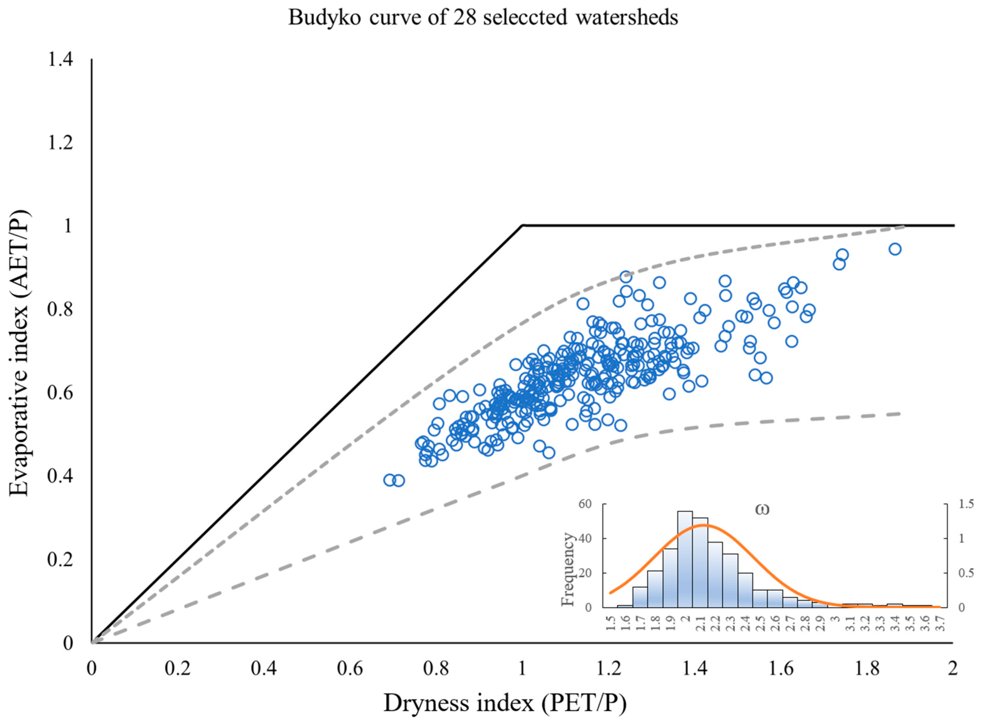
2.1. Budyko Model and Fu’s Equation

In this study, the Budyko model is used in combination with remote sensing data for $AET$ estimation. The Budyko model uses a single-parameter ($\mathsf{\omega }$) equation to describe the interconnections among $AET$, $PET$, and $P$. Over the past five decades, several empirical equations have been formulated to model the Budyko curve, drawing upon theoretical research and case studies of regional water balance. Among these equations, Fu’s equation [31] stands out as a widely used version of the Budyko model. It describes the balance between water available for runoff and water lost through evapotranspiration as expressed below (Equation (1)):

$${\displaystyle \frac{AET}{P}}=1+{\displaystyle \frac{PET}{P}}-{\left[1+{\left({\displaystyle \frac{PET}{P}}\right)}^{\omega }\right]}^{1/\omega }$$

(1)

The $\mathsf{\omega }$ value varies spatially and temporally. Based on previous studies, the value of $\mathsf{\omega }$ can be estimated from vegetation and climate variables. Although these studies provide different empirical equations for $\mathsf{\omega }$ estimation, there is no consensus on which one is the most reliable. To achieve accurate estimation of AET, four empirical equations for calculating $\mathsf{\omega }$ were tested and compared. Li, et al. [17] suggested that the value of $\mathsf{\omega }$ depends on the vegetation coverage in the watershed as follows:

$$\mathsf{\omega }=a\ast M+b$$

(2)

$$M={\displaystyle \frac{NDVI-NDV{I}_{Min}}{NDV{I}_{Max}-NDV{I}_{Min}}}$$

(3)

where $M$ is the vegetation coverage; $NDV{I}_{Max}$ and $NDV{I}_{Min}$ are the NDVI of dense forest and bare soil, respectively; $a$ and $b$ are constant coefficients. $NDV{I}_{Max}$ in this study is set to be 0.89, while $NDV{I}_{Min}$ is determined as 0.05 based on a literature analysis [18]. Th Budyko model, where $\mathsf{\omega }$ is estimated using Equations (2) and (3), is denoted as Model 1.

Ning, et al. [18] proposed that the value of $\mathsf{\omega }$ depends on vegetation coverage and a seasonal factor and can be calculated using the linear relationship shown below:

$$\mathsf{\omega }=a\ast M+b\ast S+c$$

(4)

$$S=\left|{\mathsf{\delta }}_p-{\mathsf{\delta }}_{PET}\ast {\displaystyle \frac{PE{T}_{avg}}{P_{avg}}}\right|$$

(5)

where $S$ is the seasonal factor; ${\mathsf{\delta }}_p$ is the variability of $P$, which is calculated as the difference between the maximum and minimum monthly averages of $P$; ${\mathsf{\delta }}_{PET}$ is the variability of $PET$, which is calculated as the difference between the maximum and minimum monthly averages of $PET$; $PE{T}_{avg}$ is the monthly average $PET$ in mm; $P_{avg}$ is the monthly average $P$ in mm. This Budyko model, where $\mathsf{\omega }$ is estimated using Equation (4), is denoted as Model 2.

Another study shows that $\mathsf{\omega }$ can be estimated using topographic information and vegetation data and expressed as follows [24]:

$$\mathsf{\omega }=a\ast NDVI+b\ast Lat+c\ast Long+d\ast Slope+e\ast Elev+f$$

(6)

where $Long$ is longitude in decimal degrees and $Lat$ is latitude in decimal degrees. In this study, the Budyko model that estimates $\mathsf{\omega }$ using Equation (6) is denoted as Model 3.

Additionally, there is a fourth method to estimate $\mathsf{\omega }$, using a non-linear formula as shown below [18,19].

$$a\ast M^b+e^{c\ast S}+1$$

(7)

2.2. Attribution Analysis

Attribution analysis is a tool used to identify and quantify the contributions of various factors to observed changes. It has become an increasingly popular topic in recent years as the impacts of climate change become more apparent, allowing researchers to understand the underlying causes of these changes. The value of $\mathsf{\omega }$ is linked to both climate and vegetation factors. Through $\omega$, the Budyko model captures the connection between climate and vegetation, making it a suitable model for attribution analysis. Several studies have conducted attribution analysis within the Budyko framework [32,33,34,35]. Attribution analysis can be implemented in the Budyko model to investigate the contributions of vegetation and climate factors to $AET$ changes. Previous studies carried out in Ethiopia [15], China [18,19], and Australia [22] have all suggested further investigation of attribution analysis within the Budyko framework is needed. While attribution analysis through the Budyko framework has been used to analyze the impact of climate factor changes, it has not yet been applied to any Canadian watersheds.

For a more comprehensive analysis of how different climate and land use factors could affect the changes in $AET$, an attribution analysis can be conducted. The essence of attribution analysis is to evaluate the relative contributions of $PET$, $P$, and $\mathsf{\omega }$ to the changes in $AET$ using the total differential method. The total differential method is widely regarded as a robust approach for attributing changes in the water cycle. In this method, the hydrothermal coupling parameter ($\omega$) plays a central role. The contributions of $M$ and $S$ to $AET$ are quantified by applying Fu’s equation along with the total differential method [36]. Attribution analysis is typically conducted over two time periods, enabling comparison and in-depth analysis of the changes in relative contributions. The impacts of climate change can be analyzed by considering the influence of three climatic factors, $P, PET,$ and $S$. Meanwhile, the effects of land surface change can be addressed through $M$. A change point detection analysis based on $AET$ can be first conducted to define the two time periods. This method compares the distributions before and after for every potential change point. Then, the change in $AET$ can be calculated as follows [18]:

$$\Delta AET={\displaystyle \frac{\partial AET}{\partial P}}\Delta P+{\displaystyle \frac{\partial AET}{\partial PET}}\Delta PET+{\displaystyle \frac{\partial AET}{\partial \mathsf{\omega }}}\Delta \mathsf{\omega }$$

(8)

where $\Delta AET, \Delta P, \Delta PET$ are the change in $AET, P,$ and, $PET$ between the two time periods, respectively; ${\displaystyle \frac{\partial AET}{\partial P}},{\displaystyle \frac{\partial AET}{\partial PET}},{\displaystyle \frac{\partial AET}{\partial \mathsf{\omega }}}$ are the partial derivatives of $AET$ with respect to $P$, $PET$, and $\mathsf{\omega }$.

In this study, an improved version of Equation (8), developed by Zhou, et al. [37], was used, which can be written as follows:

$$\begin{array}{c}\Delta AET=\alpha \left[{\left({\displaystyle \frac{\partial AET}{\partial P}}\right)}_1\Delta P+{\left({\displaystyle \frac{\partial AET}{\partial PET}}\right)}_1\Delta PET+\Delta \left({\displaystyle \frac{\partial AET}{\partial P}}\right)P_2+\Delta \left({\displaystyle \frac{\partial AET}{\partial PET}}\right)PE{T}_2\right]\\ \hspace{1em}\hspace{1em}\hspace{1em}\hspace{1em}\hspace{1em}\hspace{1em} +\left(1-\alpha \right){[\left({\displaystyle \frac{\partial AET}{\partial P}}\right)}_2\Delta P+{\left({\displaystyle \frac{\partial AET}{\partial PET}}\right)}_2\Delta PET+\Delta \left({\displaystyle \frac{\partial AET}{\partial P}}\right)P_1\\ \hspace{1em}\hspace{1em}\hspace{1em}\hspace{1em}\hspace{1em}\hspace{1em} +\Delta \left({\displaystyle \frac{\partial AET}{\partial PET}}\right)PE{T}_1]\end{array}$$

(9)

where $\Delta k$ is the delta between periods 1 and 2 for parameter $k$, ${\left({\displaystyle \frac{\partial h}{\partial j}}\right)}_i$ is the partial derivative of factor $j$ with respect to variable $h$ for the period $i$; $\mathsf{\alpha }$ determines the weights of periods 1 and 2’s influences on the attribution analysis results. According to Zhou, et al. [37], an $\mathsf{\alpha }$ value of 0.5 is recommended and was adopted for this study.

Subsequently, the contributions of $PET$, $P$, and $\mathsf{\omega }$ can be calculated as:

$$C_P=\mathsf{\alpha }\left[{\left({\displaystyle \frac{\partial AET}{\partial P}}\right)}_1\Delta P\right]+\left(1-\mathsf{\alpha }\right)\left[{\left({\displaystyle \frac{\partial AET}{\partial P}}\right)}_2\Delta P\right]$$

(10)

$$C_{PET}=\mathsf{\alpha }\left[{\left({\displaystyle \frac{\partial AET}{\partial PET}}\right)}_1\Delta PET\right]+\left(1-\mathsf{\alpha }\right)\left[{\left({\displaystyle \frac{\partial AET}{\partial PET}}\right)}_2\Delta PET\right]$$

(11)

$$\begin{array}{c}{C}_{\mathsf{\omega }}=\mathsf{\alpha }\left[P_2\Delta \left({\displaystyle \frac{\partial AET}{\partial P}}\right)+PE{T}_2\Delta \left({\displaystyle \frac{\partial AET}{\partial PET}}\right)\right]\\ \hspace{1em} +\left(1-\mathsf{\alpha }\right)\left[P_1\Delta \left({\displaystyle \frac{\partial AET}{\partial P}}\right)+PE{T}_1\Delta \left({\displaystyle \frac{\partial AET}{\partial PET}}\right)\right]\end{array}$$

(12)

The relative contribution can be obtained by:

$$R{C}_P={\displaystyle \frac{C_P}{\Delta AET}}$$

(13)

$$R{C}_{PET}={\displaystyle \frac{C_{PET}}{\Delta AET}}$$

(14)

where $R{C}_m$ (i.e., $R{C}_P$ and $R{C}_{PET}$) is the relative contribution of variable $m$ (i.e., $P$ and $PET$) to $AET$ changes.

Additionally, the contribution of $\mathsf{\omega }$ to $AET$ changes can be decomposed into the relative contributions of $M$ and $S$ [18]:

$${\Delta }_{\mathsf{\omega }}={\displaystyle \frac{\partial \mathsf{\omega }}{\partial M}}{\Delta }_M+{\displaystyle \frac{\partial \mathsf{\omega }}{\partial S}}{\Delta }_S$$

(15)

The relative contributions of $M$ and $S$ to $AET$ change can be calculated as:

$$R{C}_M^{\omega }={\displaystyle \frac{\frac{\partial \omega }{\partial M}{\Delta }_M}{\frac{\partial \omega }{\partial M}{\Delta }_M+\frac{\partial \omega }{\partial S}{\Delta }_S}}$$

(16)

$$R{C}_S^{\mathsf{\omega }}={\displaystyle \frac{\frac{\partial \mathsf{\omega }}{\partial S}{\Delta }_S}{\frac{\partial \mathsf{\omega }}{\partial M}{\Delta }_M+\frac{\partial \mathsf{\omega }}{\partial S}{\Delta }_S}}$$

(17)

$$C_M=C_{\mathsf{\omega }}\ast R{C}_M$$

(18)

$$C_S=C_{\mathsf{\omega }}\ast R{C}_S$$

(19)

$$R{C}_M={\displaystyle \frac{C_M}{\Delta AET}}$$

(20)

$$R{C}_S={\displaystyle \frac{C_S}{\Delta AET}}$$

(21)

where $R{C}_M^{\omega }$ and $R{C}_S^{\omega }$ are the relative contributions of $M$ and $S$ to the change in $\mathsf{\omega },\mathrm{r}\mathrm{e}\mathrm{s}\mathrm{p}\mathrm{e}\mathrm{c}\mathrm{t}\mathrm{i}\mathrm{v}\mathrm{e}\mathrm{l}\mathrm{y}.$

3. Study Area and Data

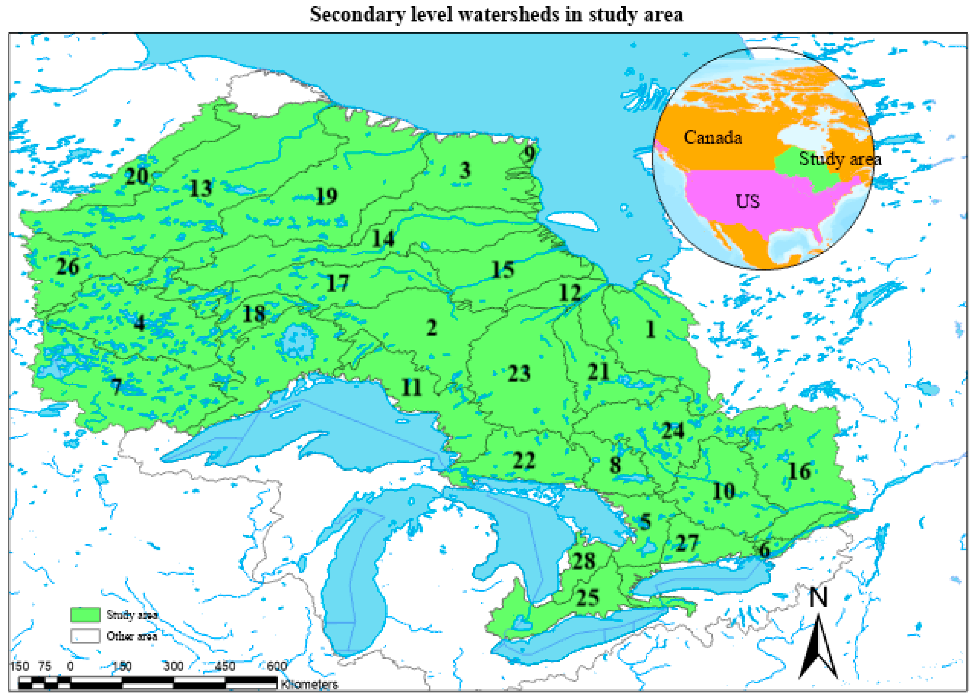
3.1. Study Area

The Province of Ontario has an area of $1.07$ × ${10}^6 \mathrm{k}{\mathrm{m}}^2$ with a population of 13.45 million (2016 census), accounting for approximately 38% of the total population of Canada [38]. The Great Lakes have a moderating effect, reducing temperature extremes in regions close to the lakes, leading to milder winters and cooler summers compared to inland areas.

In this study, a total of 36 watersheds across Ontario were initially selected (English River and Nelson River were treated as one combined watershed in this study). Among the 36 watersheds, five corresponded to the water bodies of the Great Lakes, while the other three watersheds lacked sufficient data. Consequently, these eight watersheds were removed, resulting in a total of 28 watersheds for the hydrological analysis and attribution analysis in this study, as shown in Figure 1 and

Table 1. Characteristics of 28 watersheds in Ontario.

Watershed Number	Watershed Name	Watershed Area (km2)	Latitude (Degree)	Longitude (Degree)	Slope	Elevation (m)
1	Harricanaw River-Coast	42,700	49.84	−79.12	0.25	214.3
2	Kenogami River	48,400	50.12	−85.29	0.24	255.3
3	Ekwan River-Coast	44,500	54.04	−84.29	0.14	86.0
4	English River and Nelson River	64,600	50.76	−92.08	0.37	399.8
5	Eastern Georgian Bay	19,800	44.96	−79.49	0.54	309.3
6	Upper St.Lawrence River	7400	44.76	−75.42	0.24	80.6
7	Winnipeg River	74,300	48.72	−93.04	0.34	397.5
8	Wanipitai River and French River	19,600	46.55	−80.26	0.57	306.7
9	Western James Bay Shoreline	7700	53.16	−81.84	0.05	10.2
10	Central Ottawa River	40,600	45.92	−77.42	0.88	316.1
11	Northeastern Lake Superior	36,100	48.98	−86.02	0.85	385.6
12	Moose River	18,100	50.77	−81.33	0.11	104.9
13	Severn River	100,000	53.9	−91.04	0.13	218.4
14	Attawapiskat River-Coast	57,200	52.38	−86.75	0.11	189.3
15	Lower Albany River-Coast	40,200	51.72	−83.17	0.07	80.4
16	Lower Ottawa River	55,000	46.45	−75.43	0.98	295.1
17	Upper Albany River	39,200	51.34	−87.48	0.16	248.6
18	Northwestern Lake Superior	14,000	49.85	−89.34	0.55	393.6
19	Winisk River-Coast	4400	53.77	−87.84	0.11	151.5
20	Hayes River	76,300	54.53	−92.23	0.16	202.0
21	Abitibi River	22,900	49.07	−80.54	0.29	258.2
22	Northern Lake Huron	32,800	46.74	−82.6	0.72	374.6
23	Missinaibi River and Mattagami River	60,300	48.98	−82.6	0.29	286.7
24	Upper Ottawa River	50,600	47.5	−78.73	0.62	336.3
25	Northern Lake Erie	28,700	42.94	−81.7	0.2	257.3
26	Eastern Lake Winnipeg	27,000	51.72	−94.32	0.21	353.6
27	Northern Lake Ontario and Niagara River	25,500	44.21	−78.38	0.54	266.8
28	Eastern Lake Huron	10,800	43.97	−81.11	0.33	278.9

. While $AET$ modeling results can be validated using in situ measurement data, such data are extremely sparse in the study area and are not sufficient for validating the Budyko modeling results. Therefore, the application of the Budyko framework in this study is demonstrated using MODIS data, which has been successfully used in previous studies [15,19,39,40].

3.2. Data Collection

Daily precipitation data (mm/day) from 2010 to 2020 were collected from the Integrated Multi-Satellite Retrievals for GPM (IMERG). This dataset meets the temporal and spatial requirements of this study for precipitation data. Additionally, it is not affected by compatibility issues that may arise from satellite replacements. It has a resolution of 0.1 × 0.1 degrees (10 km × 10 km). Annual precipitation data (mm/year) were calculated based on daily precipitation data from IMERG using the Geospatial Interactive Online Visualization and Analysis Infrastructure (Giovanni) [41]. The 8-day composite data of $AET$ and $PET$ from 2010 to 2020 were obtained from the MODIS global evapotranspiration product MOD16A2, with a resolution of 500 m × 500 m. Annual $AET$ and $PET$ data, which were based on MOD16A2’s 8-day composite data from 2010 to 2020, were obtained from MOD16A3 with the same resolution of 500 m × 500 m. Remote sensing-derived AET data are obtained based on the Penman-Monteith method. Monthly $NDVI$ data from 2010 to 2020 were collected from MOD13A3 with a 1000 m × 1000 m resolution, which was used to calculate the annual $NDVI$. Topographic data including the Compound Topographic Index (CTI), slope, and elevation (Elve) were obtained from the geographic database HYDRO1k, developed by the U.S. Geological Survey’s (USGS) EROS Data Center, with a resolution of 50 km × 50 km.

Table 2. Resolution of collected data.

Data	Length	Temporal Resolution	Spatial Resolution
Precipitation	2010 to 2020	daily	10 km by 10 km
AET	2010 to 2020	annually	500 m by 500 m
PET	2010 to 2020	annually	500 m by 500 m
NDVI	2010 to 2020	monthly	1000 m by 1000 m

shows the temporal and spatial resolutions of the collected data. To align the scales of different types of data in terms of temporal and spatial resolutions, a standardized process was adopted in this study. To ensure consistency, this procedure involves adjusting the spatial resolution of data to match the unit of each watershed and standardizing the temporal resolution of all data to an annual basis. Each watershed was represented by multiple cells. A representative value for each data category and each watershed was calculated by averaging the values of all cells that intersect the watershed. Subsequently, the representative values were aggregated to an annual temporal resolution by summing the daily or monthly data for subsequent calculations. The annual averages of $AET$, $PET$, and $P$ for watersheds 1 to 12 are randomly selected as example and shown in Figure 2, and the trends across all 28 watersheds are largely similar.

4. Results and Discussion

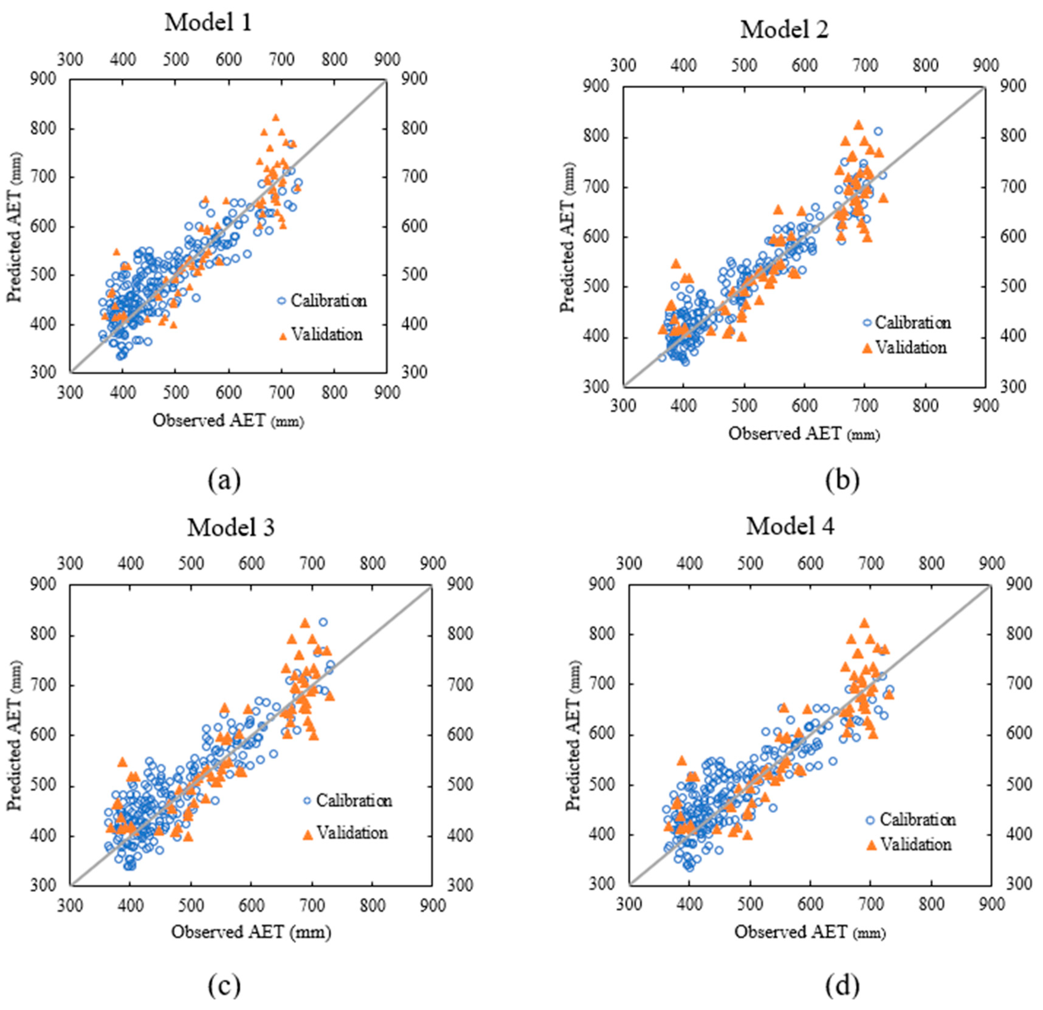
4.1. Calibration of ω

When observed data for $AET$, $P$, and $PET$ are available, the only parameter in the Budyko model, $\mathsf{\omega }$, can be calibrated (Equation (1)). In this study, a total of 308 $\mathsf{\omega }$ values are calibrated, one for each of the 28 watersheds in each of the 11 years from 2010 to 2020, shown in Figure 3. The calibrated values are marked as observed $\mathsf{\omega }$ values and then used to evaluate the four empirical estimation models, as shown in Equations (2), (4), (6), and (7). In Figure 3, the x-axis signifies the dryness index, denoting the ratio of $PET$ to $P$. This dryness index represents dry or wet conditions from the perspective of water demand. A high dryness index indicates a drier climate with a greater water demand from plants in comparison to rainfall, while a low dryness index indicates a wetter climate with a lower ratio. The y-axis represents the evaporative index, reflecting land surface conditions from the perspective of plants denoted by the ratio of $AET$ to $P$. High evaporative index indicates a wet condition with sufficient water, signifying that plants in that environment are experiencing a substantial rate of evapotranspiration. The ratio of $AET$ to $PET$ indicates dry or wet conditions based on plants’ water demand and loss. A ratio of 1 indicates a wet condition where plant water demand is fully satisfied. In this study, the majority of samples exhibit a dryness index ranging from 0.8 to 1.4 and an evaporative index ranging from 0.4 to 0.8. An evaporative index of 0.4 implies relatively low water demand in those areas, while an index of 0.8 indicates comparatively high water demand. A dryness index of 0.8 suggests relatively high rainfall, while a dryness index of 1.4 suggests relatively low rainfall in those areas. The two gray dashed lines represent the boundary values of $\mathsf{\omega }$, which are 1.5 and 3.7, respectively. All the samples form a stripe-shaped pattern in Figure 3, which is consistent with findings from previous studies [15,16,18,24]. The histogram shows that the $\mathsf{\omega }$ values follow a normal distribution slightly skewed to the right in the study area. Larger $\mathsf{\omega }$ values appear more frequently than smaller $\mathsf{\omega }$ values, which means more watersheds are sensitive to climate change.

4.2. Empirical Estimation of ω

In this study, four empirical models (Equations (2), (4), and (6)) were used to estimate $\mathsf{\omega }$. The estimated $\mathsf{\omega }$ values were used to calculate $AET$, which were then compared to the MODIS AET data (Figure 4) to evaluate the model’s performance. Among the 308 samples collected from the 28 watersheds as detailed in Section 3.1, a total of 231 samples from 21 watersheds were used for calibrating each of the four models. The remaining 77 samples from the other 7 watersheds were used for validation. To evaluate the model’s performance, Nash-Sutcliffe Efficiency (NSE) and Root Mean Square Error (RMSE) were used [42]. Mean Absolute Error (MAE), Mean Bias Error (MBE), Mean Absolute Percentage Error (MAPE), and Willmott’s Index of Agreement (d) are also used as statistical performance assessment indicators to evaluate the accuracy and bias of model predictions against observed values. For hydrologic models, an NSE value greater than 0.5 is considered to be acceptable [42].

Table 3. Performance of the four models.

Model	Calibration						Validation
	NSE	RMSE (mm)	MAE (mm)	MBE (mm)	MAPE (%)	d	NSE	RMSE (mm)	MAE (mm)	MBE (mm)	MAPE (%)	d
1	0.75	46.4	37.3	9.51	8.06	0.93	0.73	56.8	45.3	−1.16	8.33	0.91
2	0.90	32.4	25.2	5.07	5.23	0.97	0.65	66.7	54.4	10.50	10.80	0.90
3	0.79	43.2	35.2	10.00	7.66	0.95	0.74	55.5	42.7	9.27	7.89	0.94
4	0.76	45.9	36.8	9.40	7.96	0.93	0.74	55.8	44.8	0.77	8.23	0.91

presents the NSE and RMSE values for both the calibration and validation datasets on $AET$ estimation.

Model 1 estimates $\mathsf{\omega }$ values using Equation (2), which requires the least data compared to the other three models. In the calibration dataset, $AET$ tends to be overestimated when its value is below 500 mm (Figure 4a). Model 1 exhibits an NSE value of 0.75 and an RMSE value of 46.4 mm, representing the weakest goodness of fit among the four models. Despite its relatively lower accuracy during calibration, Model 1’s performance during validation is comparable to the other three models in terms of NSE and RMSE (Table 2). The results suggest that Model 1 can be used, especially for areas with limited data availability.

Models 2 and 4 estimate $\mathsf{\omega }$ values using the same input (Equations (4) and (7)). Model 4 shows satisfactory and stable performance in both the calibration and validation phases. While it requires more inputs compared to Model 1, its performance is also slightly improved. Similar to Model 1, Model 4 shows an overestimation issue for $AET$ values lower than 500 mm. The overestimation issue appears to be less significant for Model 2 (Figure 4). Among all four models, Model 2 has the highest NSE value of 0.90 and the lowest RMSE value of 32.4 mm during calibration. However, in validation, Model 2’s NSE value drops to 0.65 and its RMSE value rises to 54.4 mm, making it the lowest in validation performance in both metrics. Because the calibration and validation data are from different watersheds, the results indicate that when Model 2 is calibrated with data from certain watersheds, the model’s transferability for applications in other watersheds may be limited. This implies a potential overfitting issue associated with Model 2. Thus, Model 2 should be used with caution, especially for case studies that involve multiple watersheds.

Model 3 requires five inputs to estimate $\mathsf{\omega }$ as shown in Equation (6). Given that four out of the five inputs are single constant values, its data requirements can be considered lower than those of Models 2 and 4, yet slightly higher than those of Model 1. Model 3 achieves NSE values of 0.79 and 0.74 for calibration and validation, respectively, which are slightly better than Model 4 (0.76 and 0.74). The RMSE values for Model 3 are 43.2 mm and 55.5 mm for calibration and validation, respectively, slightly lower than those of Model 4. It is worth mentioning that the topographic variables used in Model 3 are sensitive to data resolution. In this study, the data resolution of 50 km × 50 km worked well, but the uncertainty associated with data resolution needs further investigation.

4.3. Climate and Vegetation Contributions

To further analyze the contributions of climate and vegetation factors to changes in $AET$, a change point detection analysis was first conducted [43]. Change point detection revealed that the change point occurred in the 5th year of the dataset. Consequently, the study period was partitioned into two periods: 2010 to 2015 (period 1) and 2016 to 2020 (period 2), for attribution analysis.

The changes in $AET$ and its contributing factors over the two periods are shown in

Table 4. Variable changes before and after the change point of 2015.

ID	Change from 2010 Through 2015 to 2016 to 2020
	ΔAET (mm)	ΔPET (mm)	ΔP (mm)	ΔM	ΔS
1	−6.63	−60.04	4.83	0.01	−0.05
2	1.78	−41.44	−58.36	0.01	−0.16
3	−15.21	−52.02	−21.14	0.01	0.49
4	0.16	−33.22	−31.48	−0.02	0.47
5	−8.02	−58.74	−27.39	−0.01	0.13
6	−10.43	−49.26	−2.36	−0.01	0.03
7	−13.03	−30.87	−13.11	0	0.19
8	−4.39	−66.37	−34.65	−0.01	−0.14
9	−15.54	−44.41	−29.76	0	0.39
10	−4.56	−55.44	49.29	0	0.06
11	−7.8	−52.58	56.72	0	−0.06
12	−4.81	−58.21	−33.17	0.02	−0.1
13	−4.8	−25.73	23.98	0.01	0.36
14	−0.6	−57.9	9.01	0.01	0.16
15	−6.54	−56.15	−85.88	0.02	−0.07
16	−6.07	−50.98	86.42	0.01	−0.25
17	4.92	−54.58	−45.91	0	−0.12
18	−4.4	−50.02	−10.46	−0.01	−0.3
19	−5.98	−55.1	50.41	0.01	0.46
20	−7.23	−18.21	20.57	0.01	0.27
21	−2.67	−53.38	13.74	0.02	−0.15
22	−8.05	−59.25	78.74	−0.01	−0.37
23	−2.88	−43.83	42.85	0.01	−0.22
24	−3.82	−58.9	1.6	0.01	−0.23
25	9.34	−44.89	−43.01	0.01	0.02
26	−8.8	−24.45	−57.53	−0.01	0.32
27	−5.52	−52.53	19.5	0	0.09
28	−3.38	−52.69	−15.06	0.01	0.01

. The zero values in Table 4 denote small changes (<0.01 mm) rather than actual zeros. The changes in $AET$ can be affected by $PET$, $P$, and $\mathsf{\omega }$, and the change caused by $\mathsf{\omega }$ is due to the change in $M$ and $S$. The contribution of $PET$, $P$, and $\mathsf{\omega }$ are shown in Table 4, where a larger magnitude of contribution indicated a stronger impact on $AET$ change. Furthermore, Models 2 and 4 were used for understanding the contributions of $M$ and $S$ to $\mathsf{\omega }$ using attribution analysis.

Table 5. Contribution to AET changes.

ID	C P (mm)	C PET (mm)	C ω (mm)	C M_Model 2 (mm)	C S_Model 2 (mm)	C M_Model 4 (mm)	C S_Model 4 (mm)
1	1.29	−17.8	2.49	2.92	−0.43	2.94	−0.46
2	−18.61	−10.92	25.56	*	*	*	*
3	−6.55	−17.49	18.15	3.83	14.32	5.06	13.09
4	−11.88	−6.91	18.99	*	*	*	*
5	−9.58	−17.16	19.27	52.4	−33.12	84.52	−65.25
6	−0.79	−15.37	7.14	9.45	−2.3	9.81	−2.66
7	−5.95	−6.16	−10.9	1.99	−12.89	1.65	−12.55
8	−10.91	−19.04	12.75	8.86	3.89	8.17	4.58
9	−11.13	−14.95	14.96	2.88	12.08	3.76	11.21
10	16.84	−15.63	−4.54	2.64	−7.18	1.65	−6.19
11	14.92	−16.31	−13.93	−34.87	20.94	−62.06	48.13
12	−10.01	−16.03	12.09	16.76	−4.68	16.98	−4.89
13	9.97	−5.33	−13.58	−3.54	−10.04	−3.84	−9.74
14	3.07	−13.55	4.07	2.49	1.57	2.56	1.5
15	−26.28	−15.48	31.82	37.72	−5.9	36.93	−5.11
16	24.21	−16.02	−14.67	41.13	−55.8	19.56	−34.23
17	−16.44	−12.44	24.55	4.87	19.68	4.7	19.85
18	−4.17	−11.38	8.93	3.12	5.81	2.84	6.09
19	17.85	−13.57	−7.7	−2.74	−4.96	−3.1	−4.59
20	10.56	−3.49	−12.68	−5.62	−7.06	−5.92	−6.76
21	4.64	−14.62	−7.68	−11.41	3.73	−12.39	4.71
22	23.25	−17.64	−34.02	−10.28	−23.74	−8.45	−25.56
23	13.99	−11.97	−28.28	35.93	−64.21	22.27	−50.55
24	0.46	−17.29	8.99	−67.37	76.35	−20.43	29.42
25	−17.23	−11.08	19.77	17.62	2.15	17.62	2.16
26	−19.84	−4.61	15.9	−17.58	33.48	−14.79	30.69
27	7.6	−14.07	0.19	−0.61	0.8	−0.31	0.5
28	−5.59	−15.77	−2.02	−1.96	−0.06	−1.95	−0.07

shows the relative contributions of all contributing factors. The results for Watersheds 2 and 4 in Table 5 and

Table 6. Relative contribution to AET changes.

ID	RC P (%)	RC PET (%)	RC M_Model 2 (%)	RC S_Model 2 (%)	RC M_Model 4 (%)	RC S_Model 4 (%)
1	−0.2	2.69	−0.44	0.07	−0.44	0.07
2	−10.47	−6.15	*	*	*	*
3	0.43	1.15	−0.33	−0.86	−0.33	−0.86
4	−72.86	−42.36	*	*	*	*
5	1.19	2.14	−10.54	8.13	−10.54	8.13
6	0.08	1.47	−0.94	0.26	−0.94	0.26
7	0.46	0.47	−0.13	0.96	−0.13	0.96
8	2.48	4.33	−1.86	−1.04	−1.86	−1.04
9	0.72	0.96	−0.24	−0.72	−0.24	−0.72
10	−3.69	3.42	−0.36	1.36	−0.36	1.36
11	−1.91	2.09	7.95	−6.17	7.95	−6.17
12	2.08	3.33	−3.53	1.02	−3.53	1.02
13	−2.08	1.11	0.8	2.03	0.8	2.03
14	−5.14	22.71	−4.29	−2.52	−4.29	−2.52
15	4.02	2.37	−5.65	0.78	−5.65	0.78
16	−3.99	2.64	−3.22	5.64	−3.22	5.64
17	−3.34	−2.53	0.96	4.03	0.96	4.03
18	0.95	2.59	−0.65	−1.39	−0.65	−1.39
19	−2.98	2.27	0.52	0.77	0.52	0.77
20	−1.46	0.48	0.82	0.94	0.82	0.94
21	−1.74	5.47	4.64	−1.76	4.64	−1.76
22	−2.89	2.19	1.05	3.17	1.05	3.17
23	−4.86	4.16	−7.74	17.56	−7.74	17.56
24	−0.12	4.53	5.35	−7.71	5.35	−7.71
25	−1.84	−1.19	1.89	0.23	1.89	0.23
26	2.25	0.52	1.68	−3.49	1.68	−3.49
27	−1.38	2.55	0.06	−0.09	0.06	−0.09
28	1.65	4.67	0.58	0.02	0.58	0.02

are not included because $M$ and $S$ have opposite effects on $\mathsf{\omega }$, which may cause inaccurate interpretation of their respective contributions.

For the majority of watersheds, climate factors exhibit a more substantial contribution to $AET$ changes than vegetation factors between 2010 and 2020. However, in a few watersheds, the contributions of vegetation factors were higher than those of climate factors. For example, Watershed 5 had the highest relative contribution of $M$. This may be because Watershed 5 experienced minimal $AET$ change during the two time periods. According to Equation (20), a low $AET$ change can result in a higher relative contribution of $M$. Similarly, in Watershed 23, where the $AET$ change is as minimal as −2.88 mm, the results indicate a substantial relative contribution of $M$ and $S$ (7.74% and 17.56%, respectively). It is worth mentioning that $M$ and $S$ can contribute to opposite changes in AET, which may lead to a small value of $C_{\mathsf{\omega }}$ with high absolute values of $C_M$ and $C_S$ in opposite signs. This was observed in the results for Watersheds 2 and 4, and the corresponding results were removed from Table 5 and Table 6 to avoid confusion.

When comparing Models 2 and 4, no significant differences were observed in the attribution analysis results as shown in Table 5 and Table 6. Although different approaches are used, the attribution analysis results remained consistent, underscoring the reliability and robustness of the selected methods. Watershed 27 has larger population, and its $AET$ dropped 5.52 mm from period 1 to period 2. This is because the contributions from changes in land use, such as urbanization and industrial activities, can be substantial. These activities often lead to increased impervious surfaces, altering local hydrology and increasing runoff while potentially decreasing AET. Watershed 27 has smaller values for ${RC}_{\mathrm{M}}$ and ${RC}_{\mathrm{S}}$ compared with other watersheds. Watersheds with smaller populations (such as Watershed 14) tend to have higher ${RC}_{\mathrm{PET}}$ than watersheds with larger populations.

Table 5 and Table 6 provide a detailed view of how various factors contribute to the changes in $AET$ across different watersheds. The trends and variability observed in Table 5 and Table 6 can be attributed to several factors, such as differences in landcover types and climate trends. Overall, climate factors such as $P$ and $PET$ tend to dominate the change of $AET$ through all 28 watersheds. According to the Ontario Dam Inventory, Northern Ontario has relatively few operational dams, particularly in Watersheds 3, 9, 13, 14, 15, 17, 19, 20, and 26, which show minor changes in $AET$ and low value in relative contributions for both climate and vegetation factors. However, when the change in $AET$ is minimal or close to zero, the relative contribution may appear inflated. Watersheds 6 and 27 include cities (Montreal, Ottawa, and the Greater Toronto Area). In these two watersheds, $M$ has a very low relative contribution (−0.94% and 0.06%) to $AET$ changes. Their climate factors have higher relative contribution than vegetation factor, but the magnitude of both climate and vegetation relative contribution is low compared with other watersheds (0.08% and 1.47% in Watershed 6, −1.38% and 2.55% in Watershed 27). This could because the $AET$ changes for Watersheds 6 and 27 are 10.43 mm and −5.52 mm, respectively, both showing minimal change. Watersheds 14 and 15 are geographically close and have comparable sizes (57,200 km² and 40,200 km², respectively). However, the relative contribution of $PET$ differs significantly between them, with a contribution of 22.71% for Watershed 14 and 2.37% for Watershed 15. Although the change in $PET$ is similar, the variation in $P$ is markedly different, leading to the disparity in relative contribution. The relative contribution of climate in Watershed 14 is significantly higher than that of vegetation factors, suggesting that Watershed 14 is more vulnerable to meteorological change. These features can contribute valuable information to Ontario’s climate change management decision-making process.

Although the developed Budyko models were able to provide satisfactory results for $AET$ estimation, it is noteworthy that model performance varied for different watersheds in the study area. Outstanding performances, with NSE values ranging from 0.84 to 0.99 and RMSE values between 9 and 37.5 mm, have been reported in previous studies [18]. This level of accuracy was achieved for some, but not all, of the 28 watersheds in this study. This may be due to the heterogeneity of the 28 watersheds across Ontario. Li, et al. [17] tested the performance of the Budyko model across 32 river basins and reached similar conclusions. Greve, et al. [16] also noted that the Budyko model performs better in large-scale analyses. However, if the area contains diverse features, further research is needed to achieve more accurate estimations.

Additionally, the differences among the four models are primarily due to the varying methods of ω estimation. Model 1 includes only one variable, and Model 3 lacks variation in its variable, making their partial derivatives infeasible. Contributions were calculated using partial derivatives for both Model 2 and Model 4, and the results show no significant variation between these models. This may be because the AET values used in the attribution analysis were derived from MODIS data. Further investigation, including the calculation of contributions using estimated ω values, will provide a deeper understanding of the models’ sensitivity to ω.

It is also noteworthy that the relative contributions of climate and vegetation factors to $AET$ changes were evaluated using a lumped modeling approach in this study. While this approach is well established in the literature, attribution analysis based on fully distributed models can also be found in the literature, especially for watersheds. For example, Abera, et al. [15] applied attribution analysis using a fully distributed model on a 1,104,300 km² watershed, finding that the relative contribution of vegetation factors to $AET$ change ranged from 25% to 75%, while climate factors ranged from −75% to 75%. The advantages and disadvantages of lumped versus fully distributed models need to be further investigated in future studies.

5. Conclusions

In this study, we evaluate the applicability and reliability of the Budyko framework for Canadian watersheds for the first time. The evaluation includes Actual Evapotranspiration ($AET$) estimation for 28 watersheds in Ontario, Canada. We test and compare four Budyko models with different parameter estimation equations. Finally, we conduct an attribution analysis to quantify the factors contributing to the changes in $AET$ within the study area from 2010 to 2020.

For all four Budyko models and across the 28 studied watersheds, the NSE values for $AET$ estimations are all higher than 0.65 during both the calibration and validation periods. The results demonstrate the applicability and advantages of the Budyko framework for the studied watersheds. The Budyko framework facilitates reliable large scale watershed analyses without extensive calibration efforts. It also uses remote sensing data in a straightforward and easy-to-implement way for hydrological modeling. The obtained empirical equations for estimating ω can be directly extended to other similar watersheds in Canada for $AET$ and streamflow modeling. This study reveals the great potential of the Budyko framework for other relevant hydrological analyses in Canadian watersheds. Additionally, the attribution analysis results show that most $AET$ changes in the study area are driven by climate factors, implying the importance of climate mitigation for activities affected by $AET$, such as agricultural practices and water resource allocation.

The Budyko model is a unique hydrological framework that easily incorporates remote sensing data, which is especially valuable for the vast number of Canadian watersheds with very limited observation data for $AET$ and/or streamflow. The developed models and the corresponding attribution analysis approach can be extended to many other Canadian watersheds to help understand changes in their hydrological processes. This study provides a valuable basis for the further application of the Budyko framework in Canada and other cold regions.

Although the Budyko model is simple and widely used, it assumes that water storage within the watersheds remains unchanged. This assumption is often true for most large watersheds but needs further validation for smaller watersheds. Furthermore, the use of field measurements in the calibration or validation processes, when accessible, enhances the overall robustness of $AET$ estimations. Additionally, it is important to acknowledge that the Fu equation utilized in this study is only one of many versions of the Budyko model. Other Budyko modeling approaches should be assessed to better understand the associated modeling uncertainty. Furthermore, with the wide array of readily available global precipitation datasets, exploring the use of alternative precipitation datasets could help assess the Budyko models’ sensitivity to input variations, thereby enhancing the reliability of their $AET$ estimates.

References

1. Gao, X.; Sun, M.; Zhao, Q.; Wu, P.; Zhao, X.; Pan, W.; Wang, Y. Actual ET modelling based on the Budyko framework and the sustainability of vegetation water use in the loess plateau. Sci. Total Environ. 2017, 579, 1550–1559. [Google Scholar] [CrossRef] [PubMed]
2. Lee, T.-Y.; Chiu, C.-C.; Chen, C.-J.; Lin, C.-Y.; Shiah, F.-K. Assessing future availability of water resources in Taiwan based on the Budyko framework. Ecol. Indic. 2023, 146, 109808. [Google Scholar] [CrossRef]
3. Van der Velde, Y.; Vercauteren, N.; Jaramillo, F.; Dekker, S.C.; Destouni, G.; Lyon, S.W. Exploring hydroclimatic change disparity via the Budyko framework. Hydrol. Process. 2014, 28, 4110–4118. [Google Scholar] [CrossRef]
4. Kuczera, G. Improved parameter inference in catchment models: 1. Evaluating parameter uncertainty. Water Resour. Res. 1983, 19, 1151–1162. [Google Scholar] [CrossRef]
5. Schultz, G.A. Remote sensing in hydrology. J. Hydrol. 1988, 100, 239–265. [Google Scholar] [CrossRef]
6. Kite, G.W.; Pietroniro, A. Remote sensing applications in hydrological modelling. Hydrol. Sci. J. 1996, 41, 563–591. [Google Scholar] [CrossRef]
7. Schmugge, T.J.; Kustas, W.P.; Ritchie, J.C.; Jackson, T.J.; Rango, A. Remote sensing in hydrology. Adv. Water Resour. 2002, 25, 1367–1385. [Google Scholar] [CrossRef]
8. Capolongo, D.; Refice, A.; Bocchiola, D.; D’addabbo, A.; Vouvalidis, K.; Soncini, A.; Zingaro, M.; Bovenga, F.; Stamatopoulos, L. Coupling multitemporal remote sensing with geomorphology and hydrological modeling for post flood recovery in the Strymonas dammed river basin (Greece). Sci. Total Environ. 2019, 651, 1958–1968. [Google Scholar] [CrossRef]
9. Han, P.; Long, D.; Han, Z.; Du, M.; Dai, L.; Hao, X. Improved understanding of snowmelt runoff from the headwaters of China’s Yangtze River using remotely sensed snow products and hydrological modeling. Remote Sens. Environ. 2019, 224, 44–59. [Google Scholar] [CrossRef]
10. Meresa, H. Modelling of river flow in ungauged catchment using remote sensing data: Application of the empirical (SCS-CN), artificial neural network (ANN) and hydrological model (HEC-HMS). Model. Earth Syst. Environ. 2019, 5, 257–273. [Google Scholar] [CrossRef]
11. Huang, Q.; Qin, G.; Zhang, Y.; Tang, Q.; Liu, C.; Xia, J.; Chiew, F.H.S.; Post, D. Using remote sensing data-based hydrological model calibrations for predicting runoff in ungauged or poorly gauged catchments. Water Resour. Res. 2020, 56, e2020WR028205. [Google Scholar] [CrossRef]
12. Xiong, J.; Abhishek Xu, L.; Chandanpurkar, H.A.; Famiglietti, J.S.; Zhang, C.; Ghiggi, G.; Guo, S.; Pan, Y.; Vishwakarma, B.D. ET-WB: Water-balance-based estimations of terrestrial evaporation over global land and major global basins. Earth Syst. Sci. Data 2023, 15, 4571–4597. [Google Scholar] [CrossRef]
13. Qiu, H.; Niu, J.; Phanikumar, M.S. Quantifying the space--time variability of water balance components in an agricultural basin using a process-based hydrologic model and the Budyko framework. Sci. Total Environ. 2019, 676, 176–189. [Google Scholar] [CrossRef] [PubMed]
14. Rango, A.; Shalaby, A.I. Operational applications of remote sensing in hydrology: Success, prospects and problems. Hydrol. Sci. J. 1998, 43, 947–968. [Google Scholar] [CrossRef]
15. Abera, W.; Tamene, L.; Abegaz, A.; Solomon, D. Understanding climate and land surface changes impact on water resources using Budyko framework and remote sensing data in Ethiopia. J. Arid. Environ. 2019, 167, 56–64. [Google Scholar] [CrossRef]
16. Greve, P.; Burek, P.; Wada, Y. Using the Budyko framework for calibrating a global hydrological model. Water Resour. Res. 2020, 56, e2019WR026280. [Google Scholar] [CrossRef]
17. Li, D.; Pan, M.; Cong, Z.; Zhang, L.; Wood, E. Vegetation control on water and energy balance within the Budyko framework. Water Resour. Res. 2013, 49, 969–976. [Google Scholar] [CrossRef]
18. Ning, T.; Li, Z.; Liu, W. Vegetation dynamics and climate seasonality jointly control the interannual catchment water balance in the Loess Plateau under the Budyko framework. Hydrol. Earth Syst. Sci. 2017, 21, 1515–1526. [Google Scholar] [CrossRef]
19. Yu, Y.; Zhou, Y.; Xiao, W.; Ruan, B.; Lu, F.; Hou, B.; Wang, Y.; Cui, H. Impacts of climate and vegetation on actual evapotranspiration in typical arid mountainous regions using a Budyko-based framework. Hydrol. Res. 2021, 52, 212–228. [Google Scholar] [CrossRef]
20. Zhang, L.; Potter, N.; Hickel, K.; Zhang, Y.; Shao, Q. Water balance modeling over variable time scales based on the Budyko framework--Model development and testing. J. Hydrol. 2008, 360, 117–131. [Google Scholar] [CrossRef]
21. Donohue, R.J.; Roderick, M.L.; McVicar, T.R. Roots, storms and soil pores: Incorporating key ecohydrological processes into Budyko’s hydrological model. J. Hydrol. 2012, 436, 35–50. [Google Scholar] [CrossRef]
22. Roderick, M.L.; Farquhar, G.D. A simple framework for relating variations in runoff to variations in climatic conditions and catchment properties. Water Resour. Res. 2011, 47. [Google Scholar] [CrossRef]
23. Dakhlaoui, H.; Ruelland, D.; Tramblay, Y.; Bargaoui, Z. Evaluating the robustness of conceptual rainfall-runoff models under climate variability in northern Tunisia. J. Hydrol. 2017, 550, 201–217. [Google Scholar] [CrossRef]
24. Xu, X.; Liu, W.; Scanlon, B.R.; Zhang, L.; Pan, M. Local and global factors controlling water-energy balances within the Budyko framework. Geophys. Res. Lett. 2013, 40, 6123–6129. [Google Scholar] [CrossRef]
25. Booty, W.; Lam, D.; Bowen, G.; Resler, O.; Leon, L. Modelling changes in stream water quality due to climate change in a southern Ontario watershed. Can. Water Resour. J. 2005, 30, 211–226. [Google Scholar] [CrossRef]
26. Darbandsari, P.; Coulibaly, P. Inter-comparison of lumped hydrological models in data-scarce watersheds using different precipitation forcing data sets: Case study of Northern Ontario, Canada. J. Hydrol. Reg. Stud. 2020, 31, 100730. [Google Scholar] [CrossRef]
27. Grillakis, M.G.; Koutroulis, A.G.; Tsanis, I.K. Climate change impact on the hydrology of Spencer Creek watershed in Southern Ontario, Canada. J. Hydrol. 2011, 409, 1–19. [Google Scholar] [CrossRef]
28. Jyrkama, M.I.; Sykes, J.F. The impact of climate change on spatially varying groundwater recharge in the grand river watershed (Ontario). J. Hydrol. 2007, 338, 237–250. [Google Scholar] [CrossRef]
29. Liu, Y.; Yang, W.; Leon, L.; Wong, I.; McCrimmon, C.; Dove, A.; Fong, P. Hydrologic modeling and evaluation of Best Management Practice scenarios for the Grand River watershed in Southern Ontario. J. Great Lakes Res. 2016, 42, 1289–1301. [Google Scholar] [CrossRef]
30. Rahman, M.; Bolisetti, T.; Balachandar, R. Hydrologic modelling to assess the climate change impacts in a Southern Ontario watershed. Can. J. Civ. Eng. 2012, 39, 91–103. [Google Scholar] [CrossRef]
31. Fu, B.P. On the calculation of the evaporation from land surface. Sci. Atmos. Sin 1981, 5, 23–31. [Google Scholar]
32. Bertola, M.; Viglione, A.; Vorogushyn, S.; Lun, D.; Merz, B.; Blschl, G. Do small and large floods have the same drivers of change? A regional attribution analysis in Europe. Hydrol. Earth Syst. Sci. 2021, 25, 1347–1364. [Google Scholar] [CrossRef]
33. Hu, J.; Ma, J.; Nie, C.; Xue, L.; Zhang, Y.; Ni, F.; Deng, Y.; Liu, J.; Zhou, D.; Li, L.; et al. Attribution Analysis of Runoff change in Min-tuo River Basin based on SWAT model simulations, china. Sci. Rep. 2020, 10, 2900. [Google Scholar] [CrossRef] [PubMed]
34. Philip, S.Y.; Kew, S.F.; Van Oldenborgh, G.J.; Anslow, F.S.; Seneviratne, S.I.; Vautard, R.; Coumou, D.; Ebi, K.L.; Arrighi, J.; Singh, R.; et al. Rapid attribution analysis of the extraordinary heatwave on the Pacific Coast of the US and Canada June 2021. Earth Syst. Dyn. 2021, 13, 1689–2022. [Google Scholar] [CrossRef]
35. Xu, J.; Gao, X.; Yang, Z.; Xu, T. Trend and attribution analysis of runoff changes in the Weihe River basin in the last 50 years. Water 2021, 14, 47. [Google Scholar] [CrossRef]
36. Zhou, S.; Yu, B.; Huang, Y.; Wang, G. The complementary relationship and generation of the Budyko functions. Geophys. Res. Lett. 2015, 42, 1781–1790. [Google Scholar] [CrossRef]
37. Zhou, S.; Yu, B.; Zhang, L.; Huang, Y.; Pan, M.; Wang, G. A new method to partition climate and catchment effect on the mean annual runoff based on the B udyko complementary relationship. Water Resour. Res. 2016, 52, 7163–7177. [Google Scholar] [CrossRef]
38. Yang, H.; Krantzberg, G.; Dong, X.; Hu, X. Environmental outcomes of climate migration and local governance: An empirical study of Ontario. Int. J. Clim. Change Strateg. Manag. 2023; ahead-of-print. [Google Scholar]
39. Koppa, A.; Alam, S.; Miralles, D.G.; Gebremichael, M. Budyko-based long-term water and energy balance closure in global watersheds from earth observations. Water Resour. Res. 2021, 57, e2020WR028658. [Google Scholar] [CrossRef]
40. Xu, X.; Li, X.; He, C.; Tia, W.; Tian, J. Development of a simple Budyko-based framework for the simulation and attribution of ET variability in dry regions. J. Hydrol. 2022, 610, 127955. [Google Scholar] [CrossRef]
41. Acker, J.G.; Leptoukh, G. Online Analysis Enhances Use of NASA Earth Science Data. Trans. Am. Geophys. Union 2017, 88, 14–17. [Google Scholar] [CrossRef]
42. Zhou, P.; Li, C.; Li, Z.; Cai, Y. Assessing uncertainty propagation in hybrid models for daily streamflow simulation based on arbitrary polynomial chaos expansion. Adv. Water Resour. 2022, 160, 104110. [Google Scholar] [CrossRef]
43. Aminikhanghahi, S.; Cook, D.J. A survey of methods for time series change point detection. Knowl. Inf. Syst. 2017, 51, 339–367. [Google Scholar] [CrossRef] [PubMed]
Figure 1. Twenty-eight selected watersheds in Ontario.
Hydrology 11 00191 g001
Figure 2. Annual changes in AET, PET, and P across 12 example watersheds (2010 to 2020).
Hydrology 11 00191 g002
Figure 3. Budyko curve for the 28 watersheds.
Hydrology 11 00191 g003
Figure 4. Scatter plots of observed AET and estimated AET using (a) Model 1, (b) Model 2, (c) Model 3, and (d) Model 4.
Hydrology 11 00191 g004