
The Development of a Hydrological Method for Computing Extreme Hydrographs in Engineering Dam Projects


Abstract
1. Introduction
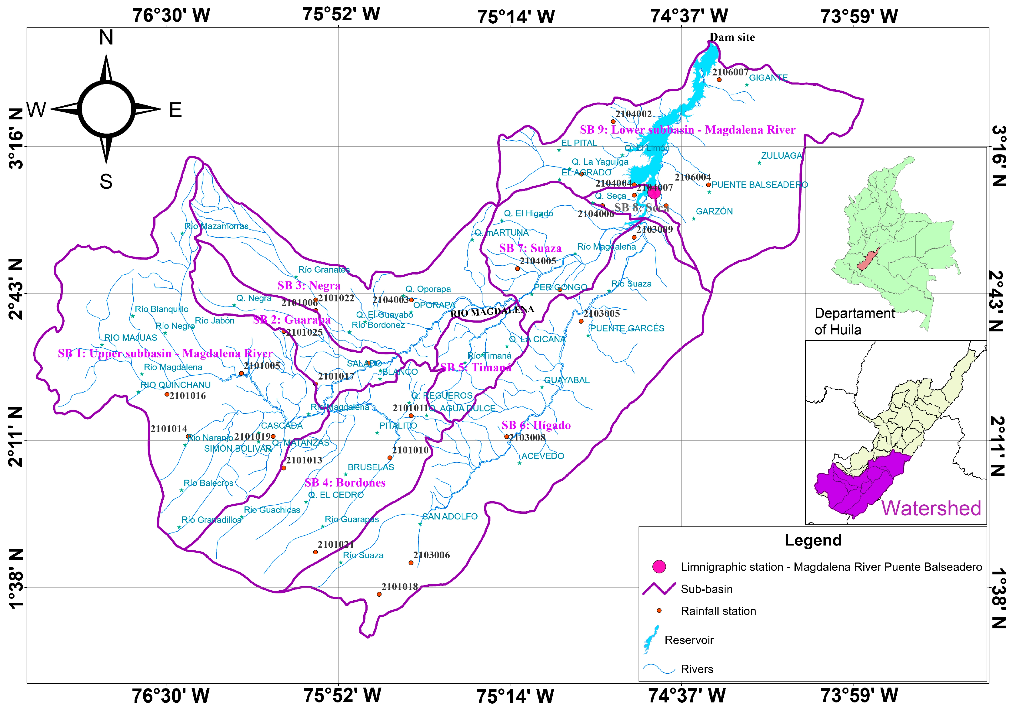
2. Case Study
3. Materials and Methods
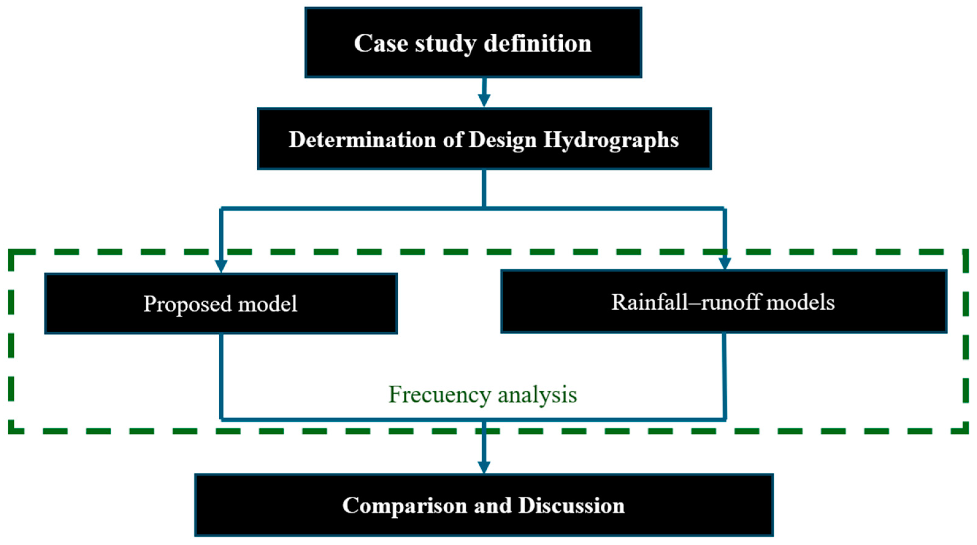
3.1. Determination of Design Hydrographs
3.1.1. Proposed Method
- Hydrological records are enough for simulating hydrographs associated with various return periods.
- The processes of the hydrological cycle for an analysed watershed are represented considering records of a hydrological station.
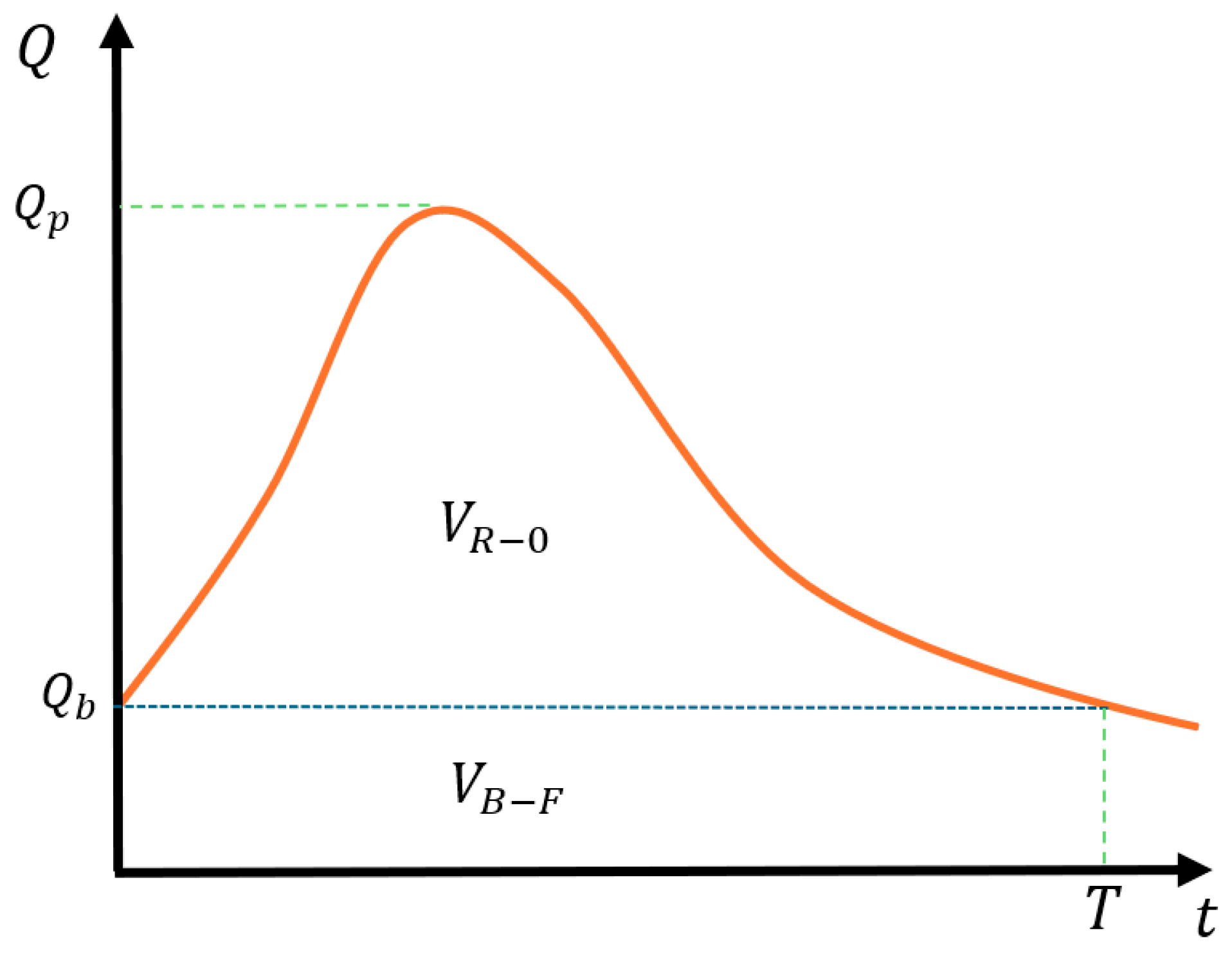
- A hydrograph can be divided into runoff and base volumes, where each one can be mathematically modelled.
- The peak flow is computed based on a frequency analysis associated with different return periods from the annual maximum flow.
- The base flow is computed based on the mean monthly flow since water level variations produced in aquifers occur slowly.
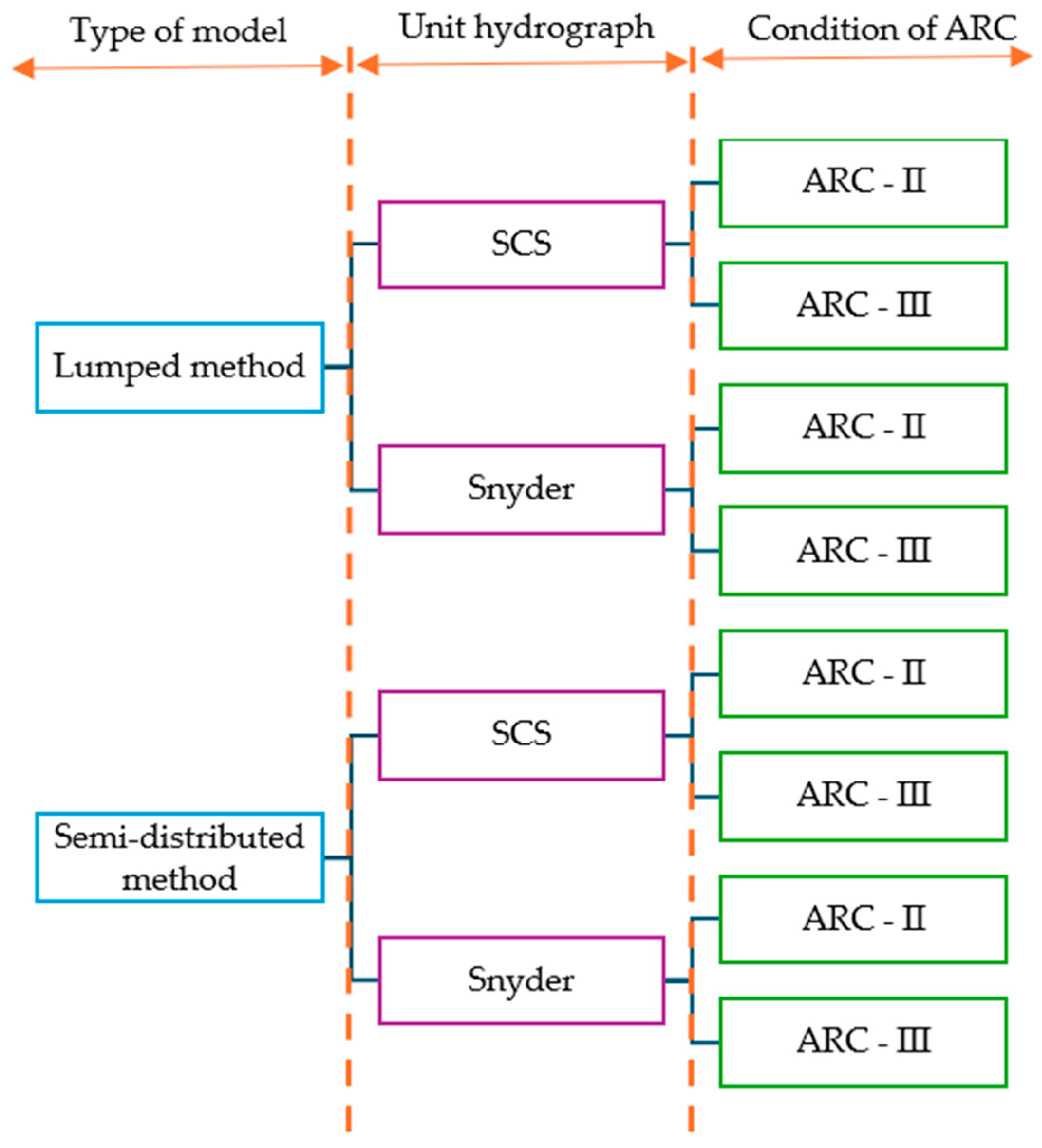
3.1.2. Rainfall–Runoff Models
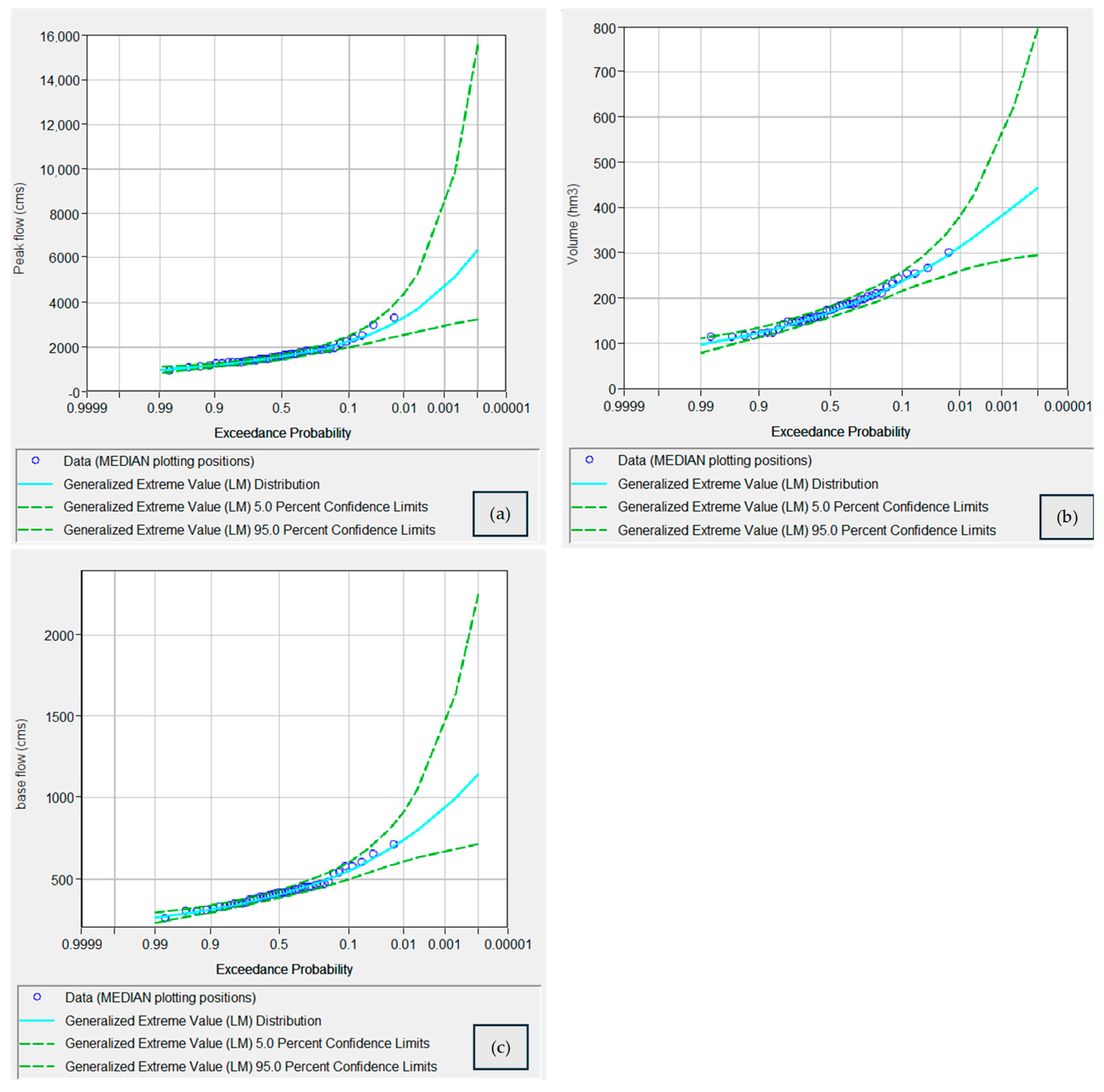
3.2. Frequency Analysis
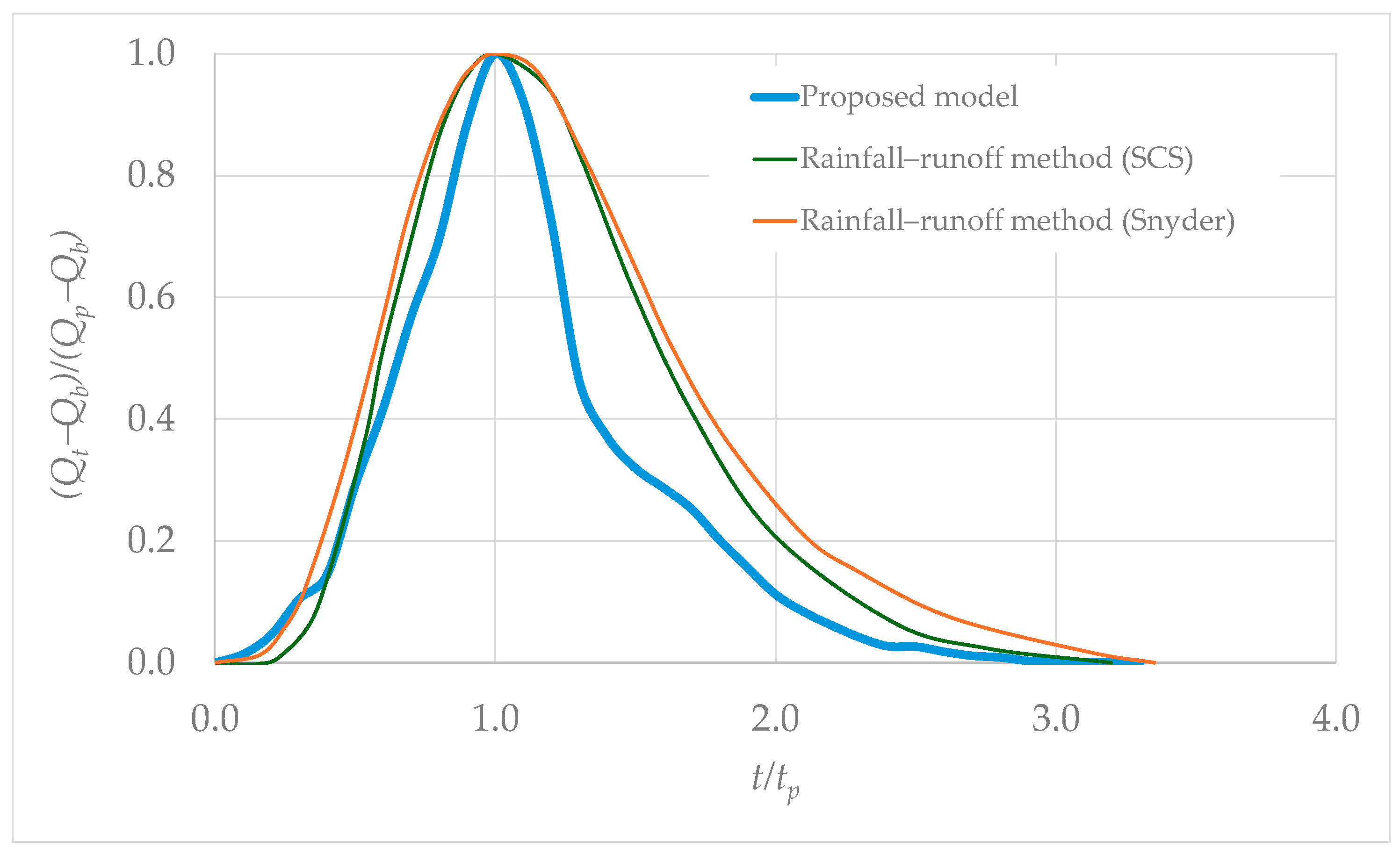
3.3. Comparison of Hydrological Methods
4. Results
4.1. Proposed Model
4.2. Computation of Rainfall–Runoff Models
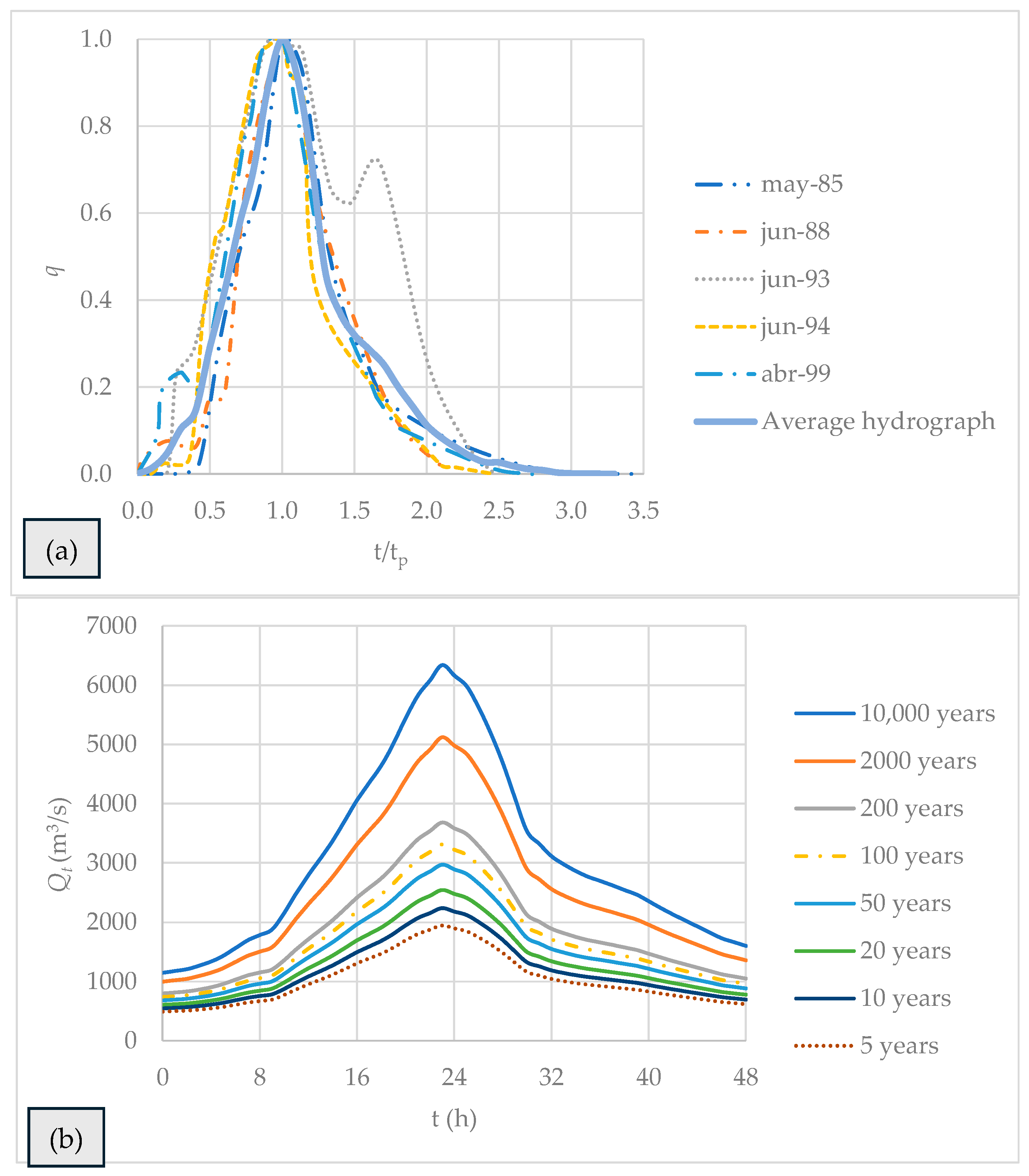
Hydrographs for Return Periods from 5 to 10,000 Years
5. Discussion
- The computed extreme peak flow, 48 h volume, and base flow series, using the GEV distribution for return periods ranging from 5 to 10,000 years, had a range of reasonable values.
- The GEV distribution using the ML method provided the best fit using the Kolmogorov–Smirnov test for all analysed series. In addition, the Chi-square test provided the best fit for the peak and base flow series, while the 48 h volume series obtained a good agreement. By comparing this with the Anderson–Darling test, the selected distribution reached the second best fit.
6. Conclusions
- The proposed model is based on hydrological records and can be used to compute design hydrographs associated with different return periods. It requires only the frequency analysis of the annual maximum series of peak flow, base flow, and water volume for various return periods and registered hydrographs.
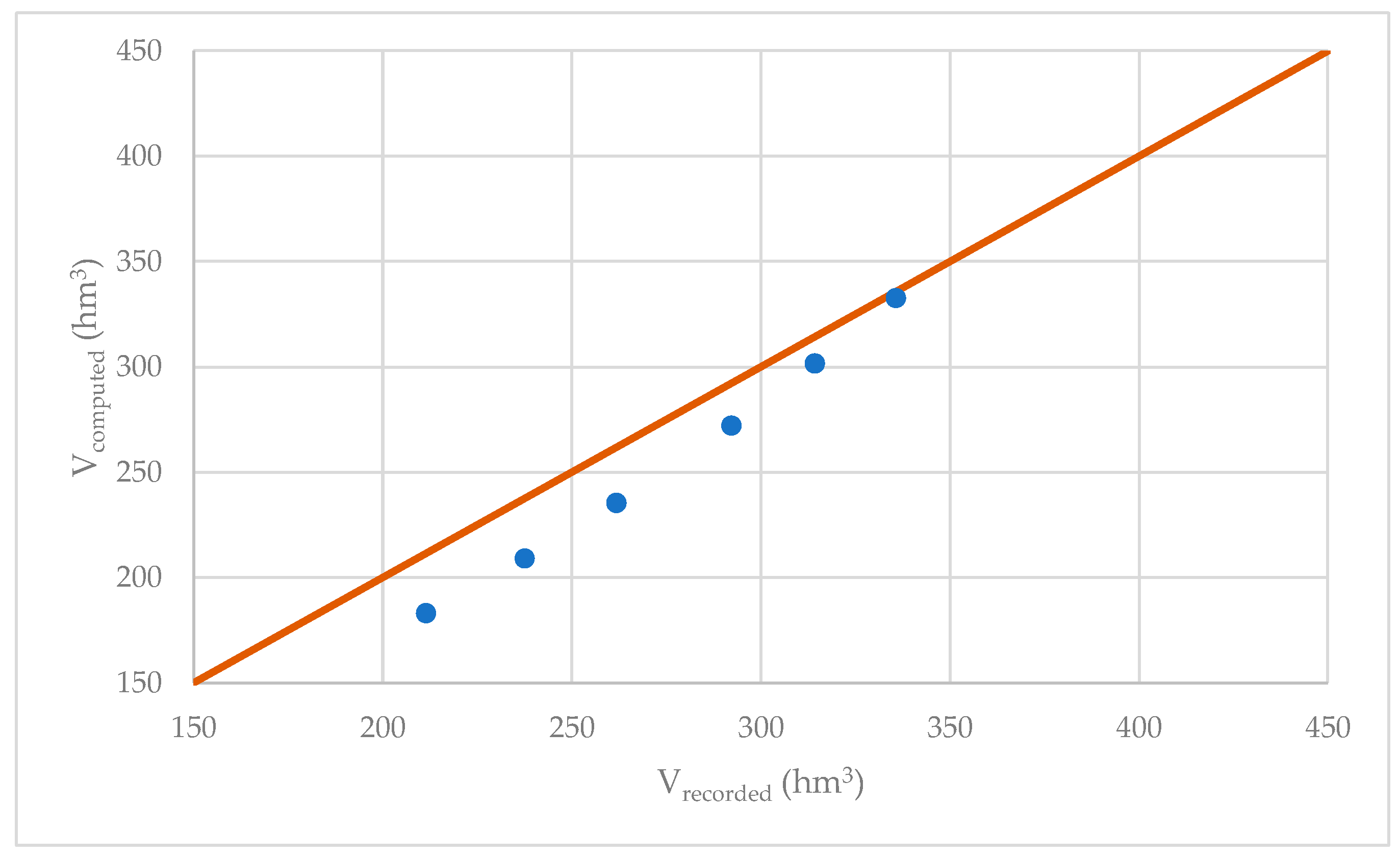
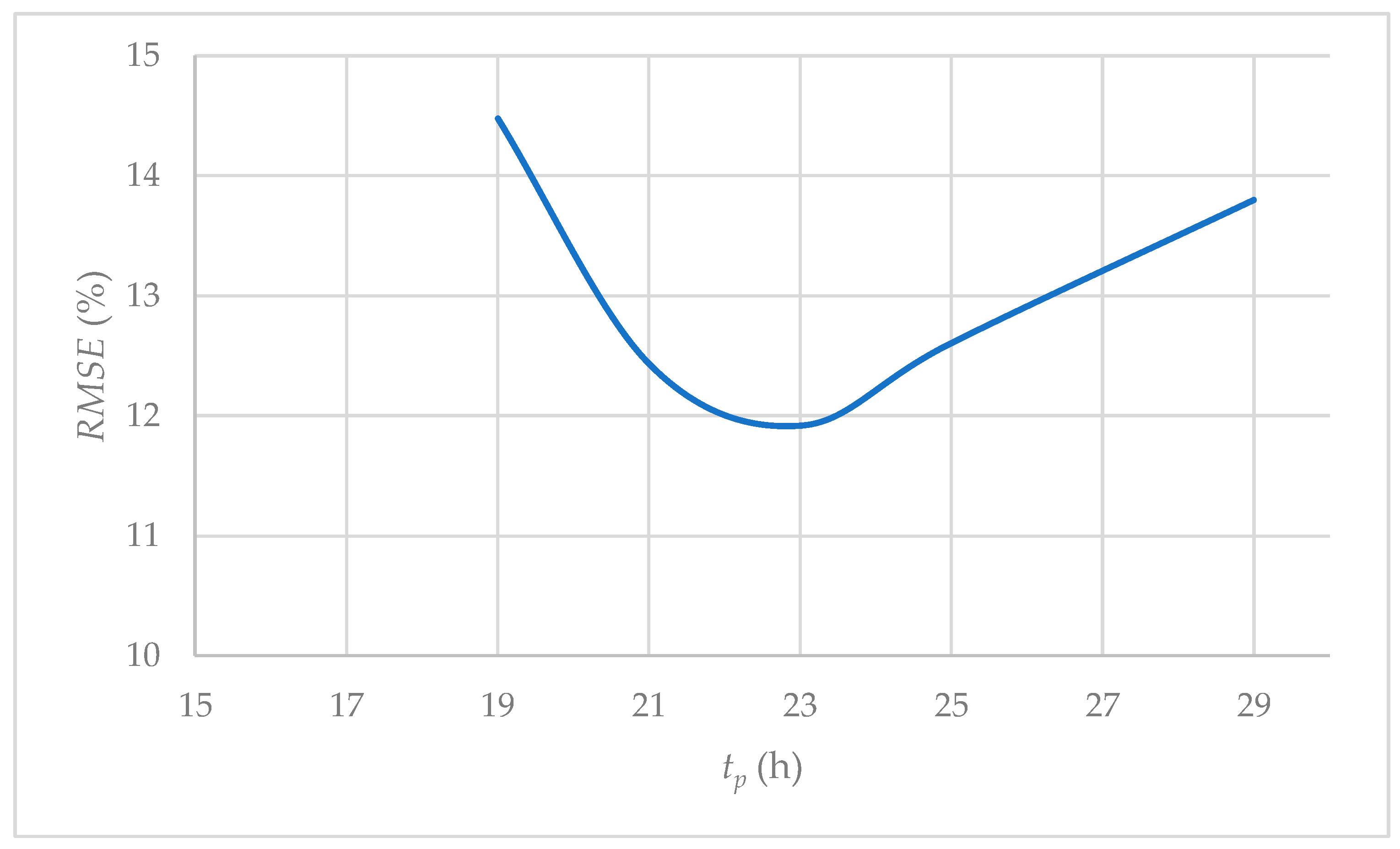
- The model was validated by comparing the computed and observed hydrograph volumes, resulting in a Root Mean Square Error () of 11.9%. This is significant as it demonstrates the method’s robustness when applied to this case study.
- The model can compute design hydrographs for various return periods, specifically for spillways and diversion structures in dam engineering projects.
- The proposed model is an innovative tool that enables faster computation of design hydrographs compared to traditional rainfall–runoff models.
Supplementary Materials
Author Contributions
Funding
Data Availability Statement
Conflicts of Interest
Appendix A

| Year | (m3/s) | (m3/s) | (hm3) | Year | (m3/s) | (m3/s) | |
|---|---|---|---|---|---|---|---|
| 1972 | 2491.4 | 602.1 | 300.9 | 1994 | 1855.4 | 444.5 | 225.3 |
| 1973 | 895.6 | 336.7 | 118.4 | 1995 | 1213.0 | 308.6 | 115.2 |
| 1974 | 2187.9 | 449.2 | 195.5 | 1996 | 1369.7 | 428.3 | 149.1 |
| 1975 | 1509.3 | 344.9 | 123.7 | 1997 | 1940.8 | 537.6 | 172.4 |
| 1976 | 1884.9 | 710.1 | 254.2 | 1998 | 1577.7 | 417.0 | 209.3 |
| 1977 | 1093.3 | 389.7 | 122.8 | 1999 | 1732.3 | 297.8 | 161.1 |
| 1978 | 1602.9 | 342.8 | 158.8 | 2000 | 3270.8 | 326.4 | 265.4 |
| 1979 | 1376.1 | 367.5 | 156.6 | 2001 | 1298.1 | 387.6 | 190.4 |
| 1980 | 1285.4 | 373.8 | 146.7 | 2002 | 1577.7 | 418.2 | 155.0 |
| 1981 | 1236.5 | 409.1 | 125.1 | 2003 | 1037.6 | 346.1 | 114.6 |
| 1982 | 1362.8 | 480.1 | 149.7 | 2004 | 1774.2 | 371.8 | 175.6 |
| 1983 | 1646.2 | 326.6 | 147.6 | 2005 | 1767.6 | 349.3 | 153.6 |
| 1984 | 1311.0 | 395.1 | 116.9 | 2006 | 1402.2 | 388.2 | 180.6 |
| 1985 | 1798.9 | 411.4 | 173.0 | 2007 | 1427.8 | 251.4 | 204.2 |
| 1986 | 2117.3 | 652.5 | 244.0 | 2008 | 2946.0 | 446.6 | 182.8 |
| 1987 | 1298.1 | 402.7 | 187.3 | 2009 | 1261.0 | 443.5 | 160.0 |
| 1988 | 1746.6 | 464.6 | 146.8 | 2010 | 1529.8 | 297.4 | 143.7 |
| 1989 | 2363.1 | 527.1 | 254.4 | 2011 | 1862.7 | 464.1 | 185.9 |
| 1990 | 1632.6 | 432.9 | 186.9 | 2012 | 1137.4 | 313.9 | 130.8 |
| 1991 | 1395.8 | 575.6 | 210.3 | 2013 | 1841.2 | 459.7 | 230.7 |
| 1992 | 1440.6 | 418.3 | 198.3 | 2014 | 1596.6 | 575.4 | 187.1 |
| 1993 | 1662.7 | 414.3 | 205.0 |
References
- Crookston, B.M.; Erpicum, S. Hydraulic Engineering of Dams. J. Hydraul. Res. 2022, 60, 184–186. [Google Scholar] [CrossRef]
- James, C.S. Spillways. In Hydraulic Structures; James, C.S., Ed.; Springer International Publishing: Cham, Switzerland, 2020; pp. 105–168. [Google Scholar] [CrossRef]
- Sharafati, A.; Doroudi, S.; Shahid, S.; Moridi, A. A Novel Stochastic Approach for Optimization of Diversion System Dimension by Considering Hydrological and Hydraulic Uncertainties. Water Resour. Manag. 2021, 35, 3649–3677. [Google Scholar] [CrossRef]
- ICOLD. Dam Failures Statistical Analysis. Bulletin 99; Commission Internationale des Grand Barrages: Paris, France, 1995. [Google Scholar]
- Aureli, F.; Maranzoni, A.; Petaccia, G. Review of Historical Dam-Break Events and Laboratory Tests on Real Topography for the Validation of Numerical Models. Water 2021, 13, 1968. [Google Scholar] [CrossRef]
- Guías Técnicas de Seguridad de Presas. Guía No 4. Avenidas de Diseño; Comité Nacional Español de Grandes Presas: Madrid, Spain, 2024; Available online: https://www.spancold.org/wp-content/uploads/2020/07/GT_04-Avenida_de_Proyecto.pdf (accessed on 20 March 2024).
- Kim, B.; Sanders, B.F. Dam-Break Flood Model Uncertainty Assessment: Case Study of Extreme Flooding with Multiple Dam Failures in Gangneung, South Korea. J. Hydraul. Eng. 2016, 142, 05016002. [Google Scholar] [CrossRef]
- Chikamori, H. Rainfall-Runoff Analysis of Flooding Caused by Typhoon RUSA in 2002 in the Gangneung Namdae River Basin, Korea. J. Nat. Disaster Sci. 2004, 26, 95–100. [Google Scholar]
- Lapointe, M.F.; Secretan, Y.; Driscoll, S.N.; Bergeron, N.; Leclerc, M. Response of the Ha! Ha! River to the Flood of July 1996 in the Saguenay Region of Quebec: Large-Scale Avulsion in a Glaciated Valley. Water Resour. Res. 1998, 34, 2383–2392. [Google Scholar] [CrossRef]
- Alcrudo, F.; Mulet, J. Description of the Tous Dam Break Case Study (Spain). J. Hydraul. Res. 2007, 45 (Suppl. 1), 45–57. [Google Scholar] [CrossRef]
- ICOLD. Selection of Design Flood. Bulletin 82; ICOLD: Paris, France, 1992. [Google Scholar]
- Collier, C.G.; Hardaker, P.J. Estimating Probable Maximum Precipitation Using a Storm Model Approach. J. Hydrol. 1996, 183, 277–306. [Google Scholar] [CrossRef]
- Jain, S.K.; Singh, V.P. Chapter 10—Reservoir Sizing. In Developments in Water Science; Jain, S.K., Singh, V.P., Eds.; Elsevier: Amsterdam, The Netherlands, 2003; Volume 51, pp. 555–612. [Google Scholar] [CrossRef]
- Jehanzaib, M.; Ajmal, M.; Achite, M.; Kim, T.-W. Comprehensive Review: Advancements in Rainfall-Runoff Modelling for Flood Mitigation. Climate 2022, 10, 147. [Google Scholar] [CrossRef]
- Rivera Trejo, F.; Escalante Sandoval, C. Análisis Comparativo de Técnicas de Estimación de Avenidas de Diseño. Ing. Del Agua 1999, 6, 49–54. [Google Scholar] [CrossRef]
- Dotson, H.W. Watershed Modeling with HEC-HMS (Hydrologic Engineering Centers-Hydrologic Modeling System) Using Spatially Distributed Rainfall. In Coping with Flash Floods; Springer: Dordrecht, The Netherlands, 2001; pp. 219–230. [Google Scholar]
- Beven, K.; Binley, A. The Future of Distributed Models: Model Calibration and Uncertainty Prediction. Hydrol. Process. 1992, 6, 279–298. [Google Scholar] [CrossRef]
- Butts, M.B.; Payne, J.T.; Kristensen, M.; Madsen, H. An Evaluation of the Impact of Model Structure on Hydrological Modelling Uncertainty for Streamflow Simulation. J. Hydrol. 2004, 298, 242–266. [Google Scholar] [CrossRef]
- Kumar, N.; Patel, P.; Singh, S.; Goyal, M.K. Understanding Non-Stationarity of Hydroclimatic Extremes and Resilience in Peninsular Catchments, India. Sci. Rep. 2023, 13, 12524. [Google Scholar] [CrossRef]
- Mustafa, N.F.; Aziz, S.F.; Ibrahim, H.M.; Abdulrahman, K.Z.; Abdalla, J.T.; Ahmad, Y.A. Double Assessment of Dam Sites for Sustainable Hydrological Management Using GIS-Fuzzy Logic and ANFIS: Halabja Water Supply Project Case Study. Iran. J. Sci. Technol. Trans. Civ. Eng. 2024. [Google Scholar] [CrossRef]
- Mishra, S. Uncertainty and Sensitivity Analysis Techniques for Hydrologic Modeling. J. Hydroinformatics 2009, 11, 282–296. [Google Scholar] [CrossRef]
- Baig, F.; Sherif, M.; Faiz, M.A. Quantification of Precipitation and Evapotranspiration Uncertainty in Rainfall-Runoff Modeling. Hydrology 2022, 9, 51. [Google Scholar] [CrossRef]
- Cu Thi, P.; Ball, J.E.; Dao, N.H. Uncertainty Estimation Using the Glue and Bayesian Approaches in Flood Estimation: A Case Study—Ba River, Vietnam. Water 2018, 10, 1641. [Google Scholar] [CrossRef]
- Shin, M.-J.; Kim, C.-S. Analysis of the Effect of Uncertainty in Rainfall-Runoff Models on Simulation Results Using a Simple Uncertainty-Screening Method. Water 2019, 11, 1361. [Google Scholar] [CrossRef]
- Ingetec, S.A. Proyecto Hidroeléctrico El Quimbo. Informe de Crecientes Para Diseño de La Presa y Obras Anexas. Documento No. PHEQ-DPLA-DOC-0005; Emgesa: Bogotá, Colombia, 2008. [Google Scholar]
- Quintero, F.; Velásquez, N. Implementation of TETIS Hydrologic Model into the Hillslope Link Model Framework. Water 2022, 14, 2610. [Google Scholar] [CrossRef]
- Sahu, M.K.; Shwetha, H.R.; Dwarakish, G.S. State-of-the-Art Hydrological Models and Application of the HEC-HMS Model: A Review. Model. Earth Syst. Environ. 2023, 9, 3029–3051. [Google Scholar] [CrossRef]
- Obeysekera, J.; Salas, J.D. Frequency of Recurrent Extremes under Nonstationarity. J. Hydrol. Eng. 2016, 21, 04016005. [Google Scholar] [CrossRef]
- Kauermann, G.; Küchenhoff, H.; Heumann, C. Multivariate and Extreme Value Distributions. In Statistical Foundations, Reasoning and Inference: For Science and Data Science; Kauermann, G., Küchenhoff, H., Heumann, C., Eds.; Springer International Publishing: Cham, Switzerland, 2021; pp. 257–281. [Google Scholar] [CrossRef]
- Abdulali, B.A.A.; Abu Bakar, M.A.; Ibrahim, K.; Mohd Ariff, N. Extreme Value Distributions: An Overview of Estimation and Simulation. J. Probab. Stat. 2022, 2022, 5449751. [Google Scholar] [CrossRef]
- Interagency Committee on Water Data. Guidelines for Determining Flood Flow Frequency, Bulletin 17B; U.S. Department of the Interior Geological Survey Office of Water Data Coordination: Reston, Virginia, 1982.
- England, J.F., Jr.; Cohn, T.A.; Faber, B.A.; Stedinger, J.R.; Thomas, W.O., Jr.; Veilleux, A.G.; Kiang, J.E.; Mason, R.R., Jr. Guidelines for Determining Flood Flow Frequency—Bulletin 17C; US Geological Survey: Reston, Virginia, 2019.
- Villalba-Barrios, A.F.; Coronado-Hernández, O.E.; Fuertes-Miquel, V.S.; Coronado-Hernández, J.R.; Ramos, H.M. Statistical Approach for Computing Base Flow Rates in Gaged Rivers and Hydropower Effect Analysis. Hydrology 2023, 10, 137. [Google Scholar] [CrossRef]
- Onen, F.; Bagatur, T. Prediction of Flood Frequency Factor for Gumbel Distribution Using Regression and GEP Model. Arab. J. Sci. Eng. 2017, 42, 3895–3906. [Google Scholar] [CrossRef]
- Dawley, S.; Zhang, Y.; Liu, X.; Jiang, P.; Tick, G.R.; Sun, H.G.; Zheng, C.; Chen, L. Statistical Analysis of Extreme Events in Precipitation, Stream Discharge, and Groundwater Head Fluctuation: Distribution, Memory, and Correlation. Water 2019, 11, 707. [Google Scholar] [CrossRef]
- Anghel, C.G. Revisiting the Use of the Gumbel Distribution: A Comprehensive Statistical Analysis Regarding Modeling Extremes and Rare Events. Mathematics 2024, 12, 2466. [Google Scholar] [CrossRef]
- Chen, X.; Shao, Q.; Xu, C.Y.; Zhang, J.; Zhang, L.; Ye, C. Comparative Study on the Selection Criteria for Fitting Flood Frequency Distribution Models with Emphasis on Upper-Tail Behavior. Water 2017, 9, 320. [Google Scholar] [CrossRef]

| Dam | Location | Watershed (km2) | Observed Peak Flow (m3/s) | Failure Year | Meteorological Conditions | References |
|---|---|---|---|---|---|---|
| Gangneung | South Korea | 258.7 | 3781 | 2002 | Around 900 mm of rainfall dropped in one day. | [7,8] |
| Lake Ha!Ha! | Canada | 610 | 910 | 1996 | A small low-pressure system generated a rainfall event for 58 h. | [9] |
| Noppikoski | Sweden | 520 | 600 | 1985 | The design flow was determined as the maximum observed flow with a safety factor equivalent to approximately a return period of 1000 years. | [4] |
| Tous | Spain | 17,820 | 15,000 | 1982 | Intensities around 500 mm dropped in one day. | [5,10] |
| Machhu II | India | 1930 | 14,000 | 1979 | Continuous rainfall over three consecutive days. | [4] |
| Sella Zerbino | Italy | 141 | 2500 | 1935 | A severe rainfall event was presented. | [4] |
| ID | Catchment | Drainage Area (km2) |
|---|---|---|
| 1 | Upper sub-basin—Magdalena River | 1527 |
| 2 | Guarapa | 807 |
| 3 | Negra | 292 |
| 4 | Bordones | 706 |
| 5 | Timaná | 209 |
| 6 | Hígado | 401 |
| 7 | Suaza | 1575 |
| 8 | Seca | 75 |
| 9 | Lower sub-basin—Magdalena River | 1238 |
| Total | Location of dam site | 6832 |
| Rainfall Station | Station Code | Rainfall Station | Station Code |
|---|---|---|---|
| Altamira | 2102002 | Agrado | 2104001 |
| Guadalupe | 2103005 | Gigante N | 2106007 |
| Antena TV | 2104002 | San José | 2101005 |
| El Hatillo | 2105014 | Insfopal | 2101011 |
| Acevedo | 2103008 | Pita La | 2106004 |
| El Carmen | 2113006 | Laguna La | 2101004 |
| Ins. El Belén | 2101017 | Tesalia N2 | 2105029 |
| San Adolfo | 2103006 | Bajo Frutal | 2101013 |
| Palestina | 2101010 | La Candela | 2101014 |
| Hornitos | 2101025 | Villa Fátima | 2101016 |
| La argentina | 2105006 | El Tabor | 2101018 |
| Hda. Meremberg | 2105019 | Alto del | 2101019 |
| Es Agr La Plata | 2105502 | Montecristo | 2101021 |
| Paez Paicol | 2105015 | Morelia | 2101022 |
| Yaguara | 2108003 | La Jagua | 2103009 |
| San Vicente | 2105016 | Oporapa | 2104003 |
| Sta Rosa | 2108007 | Pt Balseadero | 2104004 |
| Buenavista Hda | 2108012 | Tarqui | 2104005 |
| Totumo Hda | 2108013 | Tres esquinas | 2104006 |
| Armena La | 2108009 | Escalereta La | 2104007 |
| Mediania | 2101006 | Belalcazar | 2105007 |
| Garzón | 2106008 | Valencia | 4401503 |
| Sta Leticia | 2105027 |
| Variable | Range | Units |
|---|---|---|
| Temperature | 15.8–24.3 | °C |
| Relative humidity | 76.5–84.6 | % |
| Evaporation | 668.5–1338.2 | mm |
| Precipitation | 1049–2202 | mm |
| Hydrological Method | Advantages | Disadvantages |
|---|---|---|
| Rainfall–runoff models |
|
|
| Proposed model (based on hydrological records) |
|
|
| Catchment | Antecedent Runoff Condition (ARC) | |
|---|---|---|
| ARCII | ARCIII | |
| Upper sub-basin—Magdalena River | 78.2 | 90.0 |
| Guarapa | 75.6 | 88.6 |
| Negra | 75.7 | 89.0 |
| Bordones | 75.0 | 88.0 |
| Timaná | 78.4 | 90.5 |
| Hígado | 74.5 | 88.0 |
| Suaza | 75.5 | 88.5 |
| Seca | 79.4 | 91.0 |
| Lower sub-basin—Magdalena River | 75.0 | 88.0 |
| At dam site | 76.0 | 88.8 |
| Catchment | Rp (Year) | ||||||||
|---|---|---|---|---|---|---|---|---|---|
| 5 | 10 | 20 | 50 | 100 | 200 | 1000 | 2000 | 10,000 | |
| Upper sub-basin—Magdalena River | 81.3 | 96.5 | 111.0 | 129.9 | 143.4 | 158.0 | 190.3 | 204.0 | 236.5 |
| Guarapa | 72.2 | 83.1 | 93.5 | 107.0 | 117.1 | 127.3 | 150.7 | 160.6 | 184.1 |
| Negra | 78.2 | 93.2 | 107.4 | 126.0 | 139.2 | 153.7 | 185.5 | 199.0 | 231.0 |
| Bordones | 81.0 | 93.8 | 106.2 | 122.4 | 133.8 | 146.2 | 173.7 | 185.5 | 213.1 |
| Timaná | 78.1 | 88.2 | 98.0 | 110.7 | 120.0 | 129.3 | 151.0 | 160.6 | 182.4 |
| Hígado | 86.4 | 101.5 | 115.8 | 134.4 | 148.3 | 162.2 | 194.4 | 208.2 | 240.5 |
| Suaza | 79.8 | 92.5 | 105.4 | 121.5 | 133.4 | 145.2 | 173.0 | 185.4 | 212.7 |
| Seca | 74.3 | 86.1 | 97.6 | 112.4 | 123.4 | 134.4 | 159.8 | 170.8 | 196.2 |
| Lower sub-basin—Magdalena River | 96.2 | 108.8 | 121.0 | 137.0 | 148.8 | 160.6 | 188.0 | 199.8 | 227.0 |
| Average | 82.5 | 95.7 | 108.5 | 125.1 | 137.1 | 149.6 | 178.0 | 190.2 | 218.6 |
| Unit Hydrograph | Rp (Years) | ||||||||
|---|---|---|---|---|---|---|---|---|---|
| 10,000 | 2000 | 1000 | 200 | 100 | 50 | 20 | 10 | 5 | |
| ARCII | |||||||||
| SCS | 3592.9 | 2791.9 | 2467.6 | 1776.1 | 1501.9 | 1256.5 | 954.8 | 629.6 | 580.6 |
| Snyder | 2473.0 | 1972.1 | 1767.6 | 1325.2 | 1148.2 | 987.0 | 786.6 | 576.3 | 527.3 |
| ARCIII | |||||||||
| SCS | 6160.0 | 5054.6 | 4588.4 | 3535.8 | 3089.9 | 2672.6 | 2122.4 | 1385.8 | 1336.8 |
| Snyder | 3916.4 | 3244.2 | 2960.1 | 2319.1 | 2047.5 | 1791.0 | 1452.9 | 1013.6 | 964.6 |
| Unit Hydrograph | Rp (Years) | ||||||||
|---|---|---|---|---|---|---|---|---|---|
| 10,000 | 2000 | 1000 | 200 | 100 | 50 | 20 | 10 | 5 | |
| ARCII | |||||||||
| SCS | 3411.0 | 2715.3 | 2429.1 | 1803.8 | 1550.9 | 1321.6 | 1029.1 | 827.2 | 644.3 |
| Snyder | 2362.1 | 1918.4 | 1735.7 | 1332.5 | 1167.3 | 1016.1 | 821.7 | 685.7 | 559.1 |
| ARCIII | |||||||||
| SCS | 5286.2 | 4401.1 | 4025.4 | 3171.0 | 2805.1 | 2461.7 | 1999.4 | 1658.1 | 1323.7 |
| Snyder | 3429.8 | 2877.7 | 2643.8 | 2109.6 | 1880.9 | 1665.9 | 1375.2 | 1160.5 | 948.0 |
| Variable | Stationarity | Homogeneity | Trend | ||
|---|---|---|---|---|---|
| Dickey–Fuller | Phillips–Perron | KPSS | Pettitt | Mann–Kendall | |
| (m3/s) | Stationarity | Stationarity | Stationarity | Homogenity | No Trend |
| (m3/s) | Stationarity | Stationarity | Stationarity | Homogenity | No Trend |
| (hm3) | Stationarity | Stationarity | Stationarity | Homogenity | No Trend |
| Distribution (Fitting Method) | Test | ||
|---|---|---|---|
| Kolmogorov–Smirnov | Chi-Square | Anderson–Darling | |
| ) | |||
| Generalized Extreme Value (LM) | 0.069 | 2.581 | 0.199 * |
| Pearson III (LM) | 0.081 | 3.698 | 0.203 |
| Gumbel (LM) | 0.087 | 6.302 | 0.270 |
| Generalized Extreme Value (PM) | 0.078 | 4.814 | 0.217 |
| Pearson III (PM) | 0.079 | 3.698 | 0.284 |
| Gumbel (PM) | 0.091 | 7.047 | 0.326 |
| Generalized Extreme Value (MLE) | 0.075 | 6.302 | 0.192 |
| Gumbel (MLE) | 0.076 | 6.302 | 0.218 |
| Pearson III (MLE) | 0.092 | 8.535 | 0.320 |
| ) | |||
| Generalized Extreme Value (LM) | 0.081 | 5.558 | 0.228 * |
| Gumbel (LM) | 0.086 | 5.558 | 0.233 |
| Pearson III (LM) | Not applicable | ||
| Gumbel (PM) | 0.084 | 5.558 | 0.228 |
| Generalized Extreme Value (PM) | 0.090 | 5.558 | 0.244 |
| Pearson III (PM) | 0.093 | 5.558 | 0.292 |
| Gumbel (MLE) | 0.084 | 5.558 | 0.227 |
| Generalized Extreme Value (MLE) | 0.085 | 5.558 | 0.229 |
| Pearson III (MLE) | 0.096 | 5.558 | 0.283 |
| ) | |||
| Generalized Extreme Value (LM) | 0.063 | 5.558 * | 0.241 * |
| Pearson III (LM) | 0.066 | 5.558 | 0.234 |
| Gumbel (LM) | 0.069 | 5.558 | 0.269 |
| Pearson III (PM) | 0.065 | 5.186 | 0.241 |
| Generalized Extreme Value (PM) | 0.066 | 5.558 | 0.245 |
| Gumbel (PM) | 0.082 | 7.791 | 0.336 |
| Generalized Extreme Value (MLE) | 0.075 | 7.791 | 0.287 |
| Gumbel (MLE) | 0.076 | 7.791 | 0.296 |
| Pearson III (MLE) | 0.310 | 25.279 | 4.847 |
| Rp (Years) | Peak Flow (m3/s) | ||||||||
|---|---|---|---|---|---|---|---|---|---|
| Hydrological Method (Generalized Extreme Value (LM)) | Lumped Method | Semi-Distributed Method | |||||||
| SCS | Snyder | SCS | Snyder | ||||||
| ARC—II | ARC—III | ARC—II | ARC—III | ARC—II | ARC—III | ARC—II | ARC—III | ||
| 10,000 | 6341 | 3593 | 6160 | 2473 | 3916 | 3411 | 5286 | 2362 | 3430 |
| 2000 | 5121 | 2792 | 5055 | 1972 | 3244 | 2715 | 4401 | 1918 | 2878 |
| 200 | 3687 | 1776 | 3536 | 1325 | 2319 | 1804 | 3171 | 1333 | 2110 |
| 100 | 3316 | 1502 | 3090 | 1148 | 2048 | 1551 | 2805 | 1167 | 1881 |
| 50 | 2969 | 1257 | 2673 | 987 | 1791 | 1322 | 2462 | 1016 | 1666 |
| 20 | 2542 | 955 | 2122 | 787 | 1453 | 1029 | 1999 | 822 | 1375 |
| 10 | 2239 | 630 | 1386 | 576 | 1014 | 827 | 1658 | 686 | 1161 |
| 5 | 1946 | 581 | 1337 | 527 | 965 | 644 | 1324 | 559 | 948 |
Disclaimer/Publisher’s Note: The statements, opinions and data contained in all publications are solely those of the individual author(s) and contributor(s) and not of MDPI and/or the editor(s). MDPI and/or the editor(s) disclaim responsibility for any injury to people or property resulting from any ideas, methods, instructions or products referred to in the content. |
© 2024 by the authors. Licensee MDPI, Basel, Switzerland. This article is an open access article distributed under the terms and conditions of the Creative Commons Attribution (CC BY) license (https://creativecommons.org/licenses/by/4.0/).
Share and Cite
Coronado-Hernández, O.E.; Fuertes-Miquel, V.S.; Arrieta-Pastrana, A. The Development of a Hydrological Method for Computing Extreme Hydrographs in Engineering Dam Projects. Hydrology 2024, 11, 194. https://doi.org/10.3390/hydrology11110194
Coronado-Hernández OE, Fuertes-Miquel VS, Arrieta-Pastrana A. The Development of a Hydrological Method for Computing Extreme Hydrographs in Engineering Dam Projects. Hydrology. 2024; 11(11):194. https://doi.org/10.3390/hydrology11110194
Chicago/Turabian StyleCoronado-Hernández, Oscar E., Vicente S. Fuertes-Miquel, and Alfonso Arrieta-Pastrana. 2024. "The Development of a Hydrological Method for Computing Extreme Hydrographs in Engineering Dam Projects" Hydrology 11, no. 11: 194. https://doi.org/10.3390/hydrology11110194
APA StyleCoronado-Hernández, O. E., Fuertes-Miquel, V. S., & Arrieta-Pastrana, A. (2024). The Development of a Hydrological Method for Computing Extreme Hydrographs in Engineering Dam Projects. Hydrology, 11(11), 194. https://doi.org/10.3390/hydrology11110194