Abstract
Efficient water resource management in glacier- and snow-dominated basins requires accurate estimates of the snow water equivalent (SWE) in late winter and spring and melt onset timing and intensity. To understand the high spatio-temporal variability of snow and glacier ablation, a spatially distributed energy balance model combining satellite-based retrievals of albedo and snow cover was applied. Incoming short-wave energy, contributing to daily estimates of melt energy, was constrained by remotely sensed surface albedo for snow-covered surfaces. Fractional snow cover was used for non-glaciated areas, as it provides estimates of snow cover for each pixel to better constrain snow melt. Thus, available daily estimates of melt energy in a given area were the product of the possible melt energy and the fractional snow cover of the area or pixel for non-glaciated areas. This provided daily estimates of melt water to determine seasonal snow and glacier ablation in Iceland for the period 2000–2019. Observations from snow pits on land and glacier summer mass balance were used for evaluation, and observations from land and glacier-based automatic weather stations were used to evaluate model inputs for the energy balance model. The results show that the interannual SWE variability was generally high both for seasonal snow and glaciers. For seasonal snow, the largest SWE (>1000 mm) was found in mountainous and alpine areas close to the coast, notably in the East- and Westfjords, Tröllaskaga, and in the vicinity of glacier margins. Lower SWE values were observed in the central highlands, flatter inland areas, and at lower elevations. For glaciers, more SWE (glacier ablation) was associated with lower glacier elevations while less melt was observed at higher elevations. For the impurity-rich bare-ice areas that are exposed annually, observed SWE was more than 3000 mm.
1. Introduction
Efficient water resource management in glacier- and snow-dominated basins requires accurate estimates of the snow water equivalent (SWE) in winter and spring and of melt onset timing and intensity, among other ice, snow, and hydrological catchment properties [1,2]. Snowpack properties (e.g., depth, density, temperature) vary in space and time where point data might not correctly describe the spatial and temporal variability in complex environments [3,4]. Knowledge of the spatio-temporal distribution of snow and glacier ablation is important to accurately estimate partitioning of melt; calibrate and update hydrological models; organize operational planning (flood protection, onset of spring melt, seasonal resource assessment); and assess water resources in real-time.
As the climate in Iceland is modulated by heat transfer from the ocean and atmospheric circulations from lower latitudes to higher [5,6]. Storm tracks, predominantly from the southwest and southeast directions, play an important role in the hydrological cycle, as they bring precipitation, sustaining the formation of seasonal snow and glaciers in the highlands, decreasing with latitude [5,7]. About 10% of the land area of Iceland is covered with glaciers [8], while the central highlands, accumulating snow in winter, make up about 40% of the island (>550 m a.s.l.).
In Iceland, a system of reservoirs and diversions in the highlands collects and stores water for hydropower production, which accounts for about 70% of the total energy production in the country [9]. In an average hydrological year, large volumes of total flow for hydropower energy production originate from seasonal snow and glacier ablation [10,11]. Due to the high share of hydropower energy production in the total energy production mix, reliable understanding of and good forecasting capabilities for water resources development, both in short- and long-term aspects, are key to the efficient utilization of water resources. The fact that the current Icelandic energy system is a closed loop system, i.e., no means of importing or exporting electricity, underlines the importance of high-quality forecasting capabilities. Climate change projections indicate that various hydrological changes will be observed in Iceland [12,13]. Various flow dynamics, such as melt onset, seasonal snow mass, changes in the rain–snow transition elevation and distribution of solid precipitation both in the highlands and at glaciers are foreseen [10,12]. These projected changes will pose a challenge for operational control of water resources as forecasting in a non-stationary statistical environment is demanding [14]. These changes will also influence climate change adaptation for current energy projects, future developments, as well as refurbishments of older infrastructure [15,16]).
Historically, in Iceland, more focus has been given to observing glacier surface mass and energy balance and the associated runoff contribution than to measuring and monitoring seasonal snow, especially in the highlands. Surface mass balance data of Icelandic glaciers have been systematically collected bi-annually by a network of collaborators with institutes and stakeholders in Iceland. Data are collected from Vatnajökull, Langjökull, and Hofsjökull, where winter and summer mass balances are observed using conventional glaciological methods, with intermittent observations for Drangajökull, Mýrdalsjökull, and other smaller glaciers [17,18,19,20]. In many local municipalities, long-term observations of snow cover (binary snow cover, snow present or no snow presence) have been conducted since 1924 at manned observation sites, among other weather-related observations, operated by the Icelandic Meteorological Office (IMO [21]. Although this is the longest continuous record of snow cover in Iceland and provides insights into local snow cover in the lowlands, limited data are available for the highlands of Iceland.
SWE estimates are of more interest for resource assessment and hydrological modeling, but in situ observations of SWE from snow pillows or transects from snow courses are few, sparse, and discontinuous, providing limited capabilities to analyze and interpret annual distribution and evolution of snow through time [22,23]. The single longest continuous record of snow depth, density, and other properties of the snowpack was collected at Hvervellir, in the central highlands, from 1965 until 2004, when the site was upgraded to automatic measurements and snow observations decommissioned [24]. In many areas of the highlands that have hydropower plants under development or in operation, seasonal snow monitoring programs have been commissioned to improve understanding of snow hydrology although many have been short-lived [25,26,27]. At these sites, snow courses have been installed with one to two observations of snow depth and density each winter, although few of these sites have fully continuous data [23,28]. The data have been collected by various institutes over the years: the National Energy Authority (Orkustofnun), the Icelandic Met Office (Veðurstofa Íslands), and the National Power Company (Landsvirkjun).
First utilized by Martinec and Rango [29], the snow water equivalent reconstruction method uses space-based remote sensing of snow cover to retrospectively estimate the amount of water stored as snow for each pixel back to the last significant snowfall. The reconstruction technique has been adopted and successfully validated in many studies across various regions with various modifications and improvements and appears to be a reliable way to estimate spatial distribution of SWE [1,30,31,32]. The method provides a post-peak SWE estimate without the need for total precipitation which can be highly uncertain, especially in topographically complex regions [33,34]). The main limitation is that the reconstructed SWE can only be estimated after snow disappears on the ground, i.e., when snow disappears from a given pixel after total melt-out, limiting real-time usage.
Cline et al. [35] reconstructed SWE in a small, well-studied mountain basin in the Sierra Nevada using Landsat Thematic Mapper data to estimate fractional snow cover and spatially constant snow surface albedo decaying over time. Compared to in situ observations, the reconstructed SWE showed a non-significant difference (6%) for maximum SWE estimation. Molotch et al. [36] used basin-average albedo estimated from remotely sensed Airborne Visible/Infrared Imaging Spectroradiometer (AVIRIS) to make more accurate estimates of the timing and magnitude of snow melt than could be arrived at by common snow-age-based empirical relations for albedo. Rittger et al. [1] applied an approach for reconstructing the Sierra Nevada maritime snowpack from Moderate-Resolution Imaging Spectroradiometer (MODIS) data using the MODSCAG model for fractional snow cover and albedo [37]. The results showed that the model could accurately estimate SWE in a variety of topographic settings for a range of wet to dry years in the Sierra Nevada. Work by Schneider and Molotch [38] applied MODIS-based reconstructed SWE to improve real-time estimates of SWE in the Upper Colorado River using linear regression and in situ SNOTEL (Snow Telemetry Network) data, reporting reduced biases and slightly lower RMSE values. Bair et al. [32] applied machine learning models to estimate SWE throughout the snowmelt season for watersheds in Afghanistan using physiographic and remotely sensed information as predictors and reconstructed SWE as the target. The results report a 14% mean bias across the study period and RMSE values ranging from 46 to 48 mm, illustrating the possibility of estimating SWE during the snow season in remote mountains.
The primary objective of this study was to understand and quantify the spatio-temporal patterns of snow water equivalent and glacier ablation in Iceland using high-resolution meteorological climate forcing coupled with remotely sensed snow and ice surface albedo and fractional snow cover from the Moderate-Resolution Imaging Spectroradiometer sensor. The research objectives include investigating inter-annual variability of SWE and the general spatio-temporal characteristics of SWE for Iceland, understanding the ratio between melt contribution from seasonal snow and glacier ablation, and determining if trends and changes can be observed for the study period.
2. Study Area
The analysis of this study extends to the whole of Iceland, although the main emphasis was on catchments with glacier-fed rivers or areas that sustain a seasonal snowpack (highlands). Figure 1 shows the extent of the 17 main catchments analyzed (black), the six main glaciers investigated, and their sub-cardinal areas (red). Table 1 shows the topographic properties of the main catchments. For each catchment, topographic properties for the land-covered areas (seasonal snowpack) and glaciated area were extracted, showing the area and the mean, maximum, and minimum elevation within each catchment and the glacier ratio for each catchment, i.e., the ratio of the glacier-covered area to total catchment area. Table 2 shows similar information to that presented in Table 1 for the main catchments but for the main glaciers studied. For the larger glaciers, Vatnajökull, Langjökull, Hofsjökull, Mýrdalsjökull, and Drangajökull, smaller areas were defined to the main ice flow basins of the glaciers for detailed analysis. These delineated areas are shown with red boundary lines within each main glacier annotated with red text (e.g., NW for northwest). Glacier catchment delineation was from Magnússon et al. [39] for Drangajökull, Björnsson et al. [40,41] was used for Hofsjökull and Mýrdalsjökull, and Pálsson et al. [42,43] was used for Langjökull and Vatnajökull. The sub-areas were chosen as in Gunnarsson et al. [44].
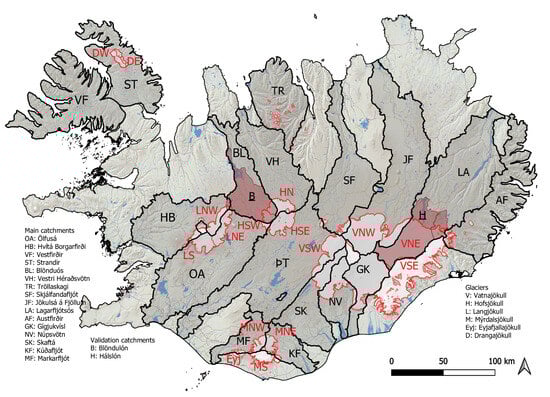

Table 1.
Topographic properties of the 17 main catchments. ID refers to Figure 1. Elevations are in meters above sea level (z). The Land and Glacier columns refer to topographic properties of the catchment divided into non-glaciated and glaciated portions. The last column, Ratio, shows the portion of catchment that is glaciated.
Table 2.
Topographic properties of the 6 main glaciers catchments and their 15 sub-areas. ID refers to Figure 1. Elevations are in meters above sea level (z). The Ratio column show the ratio of sub-glacier area to the main glacier.
3. Data and Methods
3.1. Meteorological In Situ Data
Automatic weather station (AWS) data were used to evaluate the model’s performance. For glaciers, the Icelandic Glacier Automatic Weather Stations network (ICE-GAWS) has observations from Vatnajökull, Langjökull, Hofsjökull, and Mýrdalsjökull since 1994, 2001, 2016, and 2015, respectively. Most of these stations were operated for the summer ablation season, from May out through September each year, while a few sites had data from all-year-round operation. Observations of air temperature and short- and long-wave incoming radiation were used for evaluation purposes. In total, 21 sites provided data for the study period; all sites had observations of air temperature and incoming short-wave radiation while 13 sites had data for incoming long-wave radiation. Details on data processing are provided in Gunnarsson et al. [44].
For non-glaciated areas, automatic weather stations above 250 m a.s.l. were used in the evaluation. Data were provided by the Icelandic Met Office (IMO) and observations of air temperature and short- and long-wave incoming radiation were used for evaluation purposes. There were a total of 69 sites that made air temperature observations, 7 sites where incoming short-wave radiation was available, and 6 sites where incoming long-wave radiation was available. Air temperature was measured inside a fan-aspirated radiation shield, in most cases with a PT100 probe located at 2 m height above ground. At glaciers, the height above ground can vary due to snowfall and melting of the station quad-pod. Most sites in the AWS networks used Kipp & Zonen CM14, CNR1, and CNR4 radiation sensors which have relatively uniform spectral response ranging from 0.3 to 2.8 m, with reported uncertainty ranging from 3 to 10% for daily totals over ice- and snow-covered surfaces [45,46].
For both networks (AWS and GAWS), daily averages were calculated if 20 hourly values or more were available within the day; otherwise, the observations were omitted for evaluation. Table A1 in the Appendix A provides details of the location, elevation, type of site, and number of observations for each site.
3.2. Glacier Surface Mass Balance Data
Surface mass balance data of Icelandic glaciers were systematically collected bi-annually by a network of collaborators with institutes and stakeholders in Iceland. Where winter and summer mass balance were observed, data collection was conducted by conventional glaciological methods. Shallow snow cores were drilled at selected locations in the spring to determine the density and depth of the winter snow cover. Stakes in the accumulation zone and wires or stakes in the ablation zone were left during the summer for a readout in the fall, allowing for summer mass balance estimates. For Vatnajökull and Langjökull, spatially continuous maps were derived based on dense point data [11,20], while for Hofsjökull and Mýrdalsjökull point data were available representing the main glacier outlets. These procedures for drilling and post-processing of data are described in many previous studies and annual reports of mass balance [11,17,18,20]. Data were available for Vatnajökull (glaciological years 1991/92 to 2018/19), Hofsjökull (1987/88 to 2018/19), and Langjökull (1996/97 to 2018/19). Data spanning the study period include 1227, 389, 383, and 68 surface mass balance observations for Vatnajökull, Hofsjökull, Langjökull, and Mýrdalsjökull, respectively.
3.3. Snow Cover and Albedo Data
For the SWE reconstruction model applied in this study, fractional snow-covered area (fSCA), and snow and ice surface albedo () were derived from Moderate-Resolution Imaging Spectroradiometer (MODIS) data using processing models developed for Iceland by Gunnarsson et al. [44,47]. Both products rely on the MOD10A1 (Terra satellite) and MYD10A1 (Aqua satellite) fractional snow cover (scientific data set: NDSI Snow Cover) and snow albedo (scientific data set: Snow Albedo Daily Tile) for the grid tile h17v02 covering most of Iceland, excluding a small portion of the Snæfellsnes peninsula.
For fractional snow cover, three main processing steps were applied. First, daily tiles from MOD10A1 and MYD10A1 were merged into a single daily tile with priority for Terra data due to failure in band 6 in Aqua [48]. Second, to reduce the number of cloud-obscured pixels remaining, a temporal aggregation was applied. The temporal aggregation range is set as the number of days backwards and forwards, and each center–date data point was allowed to search for classified pixel data. Priority was given to data closest to the center–date data point and from the forward date if both backward and forward dates had data. The aggregation window was 7 days. Finally, the cloud-obscured pixels remaining after daily merging and temporal aggregation were classified using a classification tree trained daily on four predicting variables: location (east, north), elevation (Z), and aspect. Further information and details are in Gunnarsson et al. [47].
For snow and ice surface albedo, the first processing steps were the same as for fSCA while the aggregation window was 11 days for temporal aggregation. The cloud-obscured pixels remaining after daily merging and temporal aggregation were classified with a daily-trained random forest model using the same predicting variables as for fSCA. Further information and details are available in Gunnarsson et al. [44].
3.4. Seasonal Snow Data
Few sites had snow field survey data available for the study period. The most extensive data were from the Setur AWS in the south-central highlands, where from 2004 to 2015, ground-based estimates of SWE were available from snow transect surveys conducted in March or April each year. Concurrently, spatial variability of the SWE was estimated on two 1 km long transects with a north–south and east–west orientation where snow depth was collected at 100 m intervals. The main snow pit for SWE location was located at the midpoint of these two transects. Since 2015, a Campbell Scientific passive CS725 snow water equivalent sensor has been operated at the site. The sensor detects the attenuation of the electromagnetic energy from the ground, and the SWE can be estimated. The CS725 estimates the SWE over an area of 50 to 100 square meters and provides a time series of SWE estimation. Snow pit data were also available from other sites spanning the study period. In total, 70 estimates of SWE collected from mid-March to mid-April were used. For the majority of observations, snow density was measured in 10 cm increments from the snow surface to the ground using a 1000 cc Snowmetric RIP1 density cutter (Kelly cutter). A combination of depth and density provides point-based SWE estimates at the site. At some sites, collections were conducted with Federal or SnowHydro samplers (coring tubes). In those cases, three to five cores were taken at each site and the average of all collections used as the mean SWE estimate.
3.5. Model Forcing
Meteorological forcing was from the RAV2 project. RAV2 is based on the Weather Research and Forecast model (WRF) version 3.6.1 coupled to the NOAH land surface model to provide climatological surface variables at a 2 km spatial resolution and 1 hour temporal resolution spanning the period from 1.9.1957 to 31.8.2019. From 1979 to 2019 the model was forced with boundary conditions from the European Centre for Medium Range Weather Forecasts (ECMWF) ERA-Interim reanalysis [49]. The model domain spans Iceland in a nested domain at a 2 km spatial resolution at the surface (326 × 256 pixels) whereas the outer domain of the model has a spatial resolution of 10 km (121 × 111 pixels). Vertical resolution is 65 levels, up to the 25 hPa level. Relevant surface data for melt calculations were extracted for use in the reconstruction model: air temperature at 2 m, surface temperature, incoming long- and short-wave radiation, surface pressure, and specific humidity; all data are re-sampled to daily average values. Further description of the RAV2 model setup and output configuration is found in [50]. Downscaling of the meteorological forcing from the 2 km RAV2 WRF grid to the 500 m MODIS grid was based on the IslandsDEM digital elevation model (DEM) from the National Land Survey of Iceland at 20 m spatial resolution (Accessed 01.06.2021). Bi-cubic interpolation was applied to regrid the DEM to the MODIS grid. Variables dependent on elevation (air temperature and long-wave radiation) were adjusted for the difference between the coarse-resolution RAV2 DEM and high-resolution IslandsDEM at 500 m using a lapse rate. Air temperature, T, was downscaled from 2 km RAV2 reanalysis data to 500 m grid cells using an environmental lapse rate of −6.5 K/km assuming a linear dependence on elevation above mean sea level uniformly across the domain outside of glaciated areas [51,52]. For glaciers, an environmental lapse rate of –7.0 K/km was used for JFMA and SOND while –5.5 K/km was applied for the active melt season, MJJA, following results from [53,54]. Downward long-wave radiation is primarily determined by humidity and temperature vertical atmospheric profiles, which correlate strongly with elevation [55,56]. In this study, no adjustments were made to account for enhancement of long-wave radiation due to terrain emission as the conditions were not general in Iceland while a lapse rate of –29 W m km was used for elevation difference adjustment. Further details on downscaling of temperature and long-wave radiation are in Gunnarsson et al. [57].
3.6. SWE Reconstruction Model
The reconstruction model adopted in the present study is based on the formulation proposed by Brubaker et al. [58] and used by Rittger et al. [1]. The formulation uses an explicit calculation for the short-wave and long-wave radiation terms and a pseudo-physically based formulation for turbulent fluxes relying on a degree day factor and temperature. The potential melt, , in mm at time j, is defined as:
where m is a conversion factor from energy to melt, 0.26 mm day per W m, R is the net radiation, is a degree day factor, and is the mean daily temperature above 273.15 K. is set to zero (no melt) when the temperature is less than or equal to 273.15 K or when fSCA is less than 10% for a given pixel.
The net radiation flux, R, is defined as:
where SW↓ is incoming solar radiation, is broadband albedo from MODIS and LW↓ and LW↑ are incoming and outgoing long-wave radiation, respectively. Outgoing long-wave radiation (LW↑) defines the radiation emitted to space by Earth’s surface and depends on surface temperature. Here, outgoing long-wave radiation is calculated based on the Stefan–Boltzman law:
where is the emissivity of snow (0.99) [59], is the Stefan–Boltzman constant and is surface temperature in Kelvin. Simple approximations have been adapted assuming surface temperature to be equal to the daily average 2 m air temperature but constrained to a maximum of 0 C and lagging 2 m air temperature in time to present surface temperature [35,60,61]. More complex methods have also been adapted, solving for the snow surface temperature as the equilibrium temperature that balances the energy exchanges [32,62,63]. Raleigh et al. [64] suggested using dew point temperature as a snow surface temperature proxy, which was adopted for further calculations in this study. Solutions for > 273.15 K indicate availability of melt energy; was set to 273.15 K and melt was computed. Otherwise, melt was set to zero.
At any time j, the available melt to melt snow and ice in a given area is the product of the potential melt and the fractional snow cover (0–1) of the area or pixel:
Fractional snow cover and albedo was based on MODIS-processed products described in Section 3.3. For glaciated areas, a constant fSCA mask at 100% snow cover was applied and glacier boundaries were kept fixed through the study period (2000–2019) using the available delineation spanning 2007–2013 from [8].
For seasonal snow, was summed from the day of snow disappearance in the MODIS fSCA data until March 15th each year. In theory, the peak SWE date can be estimated from the earliest date when melt energy was zero for an extended time in spring. In many studies ancillary information (snow pillows or other SWE sources) was used to estimate the date of peak SWE, such as station data or other field data [1,62], while in many cases no such data were available. For glaciers, snow cover was 100% during all periods and all available melt energy was summed to account for annual summer melt. For the seasonal snow maximum, SWE was determined as the maximum accumulated value for each pixel. In the case of glaciers, all calculated melt was accumulated from March 15th out through September except for 2019 where no climate forcings were available for the month of September due to the end-of-life of ERA-Interim.
In reality, glaciers melt both accumulated winter snow, firn, and ice during the melt season. In literature, daily glacier summer melt is referred to as summer ablation and the accumulated summer ablation over the melt period as summer mass balance () [65]. Here, for simplification, snow water equivalent (SWE) refers to both the reconstructed seasonal snowpack and glacier ablation. For the calculated daily melt, the calculation process was the same for glaciers and seasonal snow, with the exception of a constant full areal snow cover for glaciers.
3.7. Cold Content
Cold content is a component of the snowpack energy balance representing the internal snowpack energy deficit. This deficit must be overcome before runoff from a snowpack can occur. Cold content is a linear function of the snow water equivalent (mass) and the snowpack temperature where colder and greater SWE snowpacks have higher energy deficits [66]. Many previous reconstruction studies estimated cold content by using a proxy. Jepsen et al. [60] initialized cold content as zero at midnight each day and kept a running total of the net energy flux to the snowpack. This sum, when negative, was set to equal the magnitude of cold content. By applying this method, melt spikes during winter were reduced. Bair et al. [32] used a similar approach while resetting cold content not daily at midnight but daily after sunset.
Cold content was not modeled in this study since the density and depth of the snowpack were not known. A similar method was applied for cold content to that in [60]. For seasonal snow, daily melt energy was calculated and, if negative, applied as the pixels of the cold content for next day’s calculation. This value was updated each day if the melt energy was negative. For glaciers, generally the winter snowpack is much deeper and holds more cold content, especially at higher elevations and in the accumulation areas, compared to seasonal snow. A simple scheme based on elevation was applied where the cold content was based on a running sum over a set number of days and applied daily as the cold content to overcome. The number of days summed over was based on elevation of the pixel; thus, from 250 m a.s.l. in 250 m steps, one day was added to the sum. This means that a pixel located on a glacier at or lower than 250 m a.s.l. has the same cold content criteria as seasonal snow, while a pixel above 250 m a.s.l. and below 500 m a.s.l. sums negative energy over two days, etc. The thresholds were based on preliminary model testing but seem to have limited influence on the melt magnitude at seasonal scales.
4. Evaluation
4.1. Energy Balance Components
Figure 2 shows the comparison of the observed and modeled air temperature values, LW↓ and SW↓, for the different meteorological station locations on glaciers (GAWS) and on non-glaciated areas (AWS). Evaluation of RAV2 data is reported in more detail for glaciers in Gunnarsson et al. [57]. For the full evaluation period, April through October, the results show good agreement each year, both visually and statistically, and are within ranges reported in other studies [67]. Table 3 shows the evaluation results for the whole evaluation period (AMJJASO), similar to Figure 2, but also for individual months within the full evaluation period.
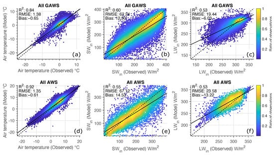
Figure 2.
Evaluation of the downscaled daily RAV2 modeled incoming solar radiation, incoming long-wave radiation, and air temperature with ground observations. (a–c) show results from weather stations operated on glaciers (GAWS) while (d–f) show results from stations outside of glaciers (AWS). Color shows the normalized (0–1) density distribution of data. Dotted black line shows 1:1, and black line shows the calculated linear fit to the data.
Table 3.
Summary statistics for observed and simulated air temperature at 2 m height, incoming short-wave radiation, and incoming long-wave radiation. Monthly and inter-seasonal variation statistics were compiled for the whole period of April through October as well as for individual months. ID refers to type of station (L for land and G for glaciers). No. Sites accounts for the number of sites used in the evaluation. Note that the number of sites column shows the number of sites used for air temperature calculations. In almost all cases, the availability of radiation observations was much lower. Refer to Table A1 for individual sites and instruments available.
The coefficient of determination (R) for air temperature ranges from 0.92 to 0.56 for glaciers with the lowest values in July and August. For stations on land, the R values were higher, ranging from 0.94 to 0.83, with less systematic bias during July and August than for sites on glaciers. Lower R values on glaciers during mid and late summer might relate to underestimation of LW↓ due to negative temperature biases. The consistent negative bias indicates that the model slightly overestimates air temperature. A similar bias was observed for the whole period for stations on land. The root mean square errors (RMSE) were similar, 1.38 C and 1.35 C, for glaciers and land. For individual months, air temperature generally had somewhat better results for sites on land than glaciers. For all sites, air temperature RMSE ranges from 0.76 to 1.25 C, with no systematic pattern for different months. The lowest values were observed in October both for land and glaciers.
For radiation, far fewer sites on land had observations of incoming short- and long-wave radiation. For short-wave radiation, the RMSE ranged from 9 to 61 W m, with the highest values occurring during summer coincident with the summer solstice. The R values range consistently from 0.41 to 0.64, and overall, the bias is positive, ranging from −3.6 to 25 W m. For long-wave radiation, agreement was good, with an RMSE from 8 to 26 W m, an R ranging from 0.55 to 0.79, and a general negative bias from −2 to −18 W m. The instrument reported uncertainty at a daily total less than 5% (∼15 W) for short-wave radiation and less than 10% (∼30 W) for long-wave radiation. Recent work by Schmidt et al. [67] reported similar results when validating HIRHAM5 for surface mass balance calculations for Vatnajökull.
4.2. Summer Mass Balance for Glaciers
Figure 3 shows the evaluation results for point summer mass balance data for Vatnajökull, Hofsjökull, Langjökull, and Mýrdalsjökull. The agreement between reconstructed SWE and observations was acceptable for Vatnajökull and poorest for Mýrdalsjökull. For Vatnajökull, 1227 observations were available within the study period, resulting in an average RMS error of 0.43 m, R as 0.94, with very low bias, only 0.02 m. Recent work by Schmidt et al. [67] using the hydrostatic RCM HIRHAM5 model with a new albedo parametrization, dependent both on snow age and surface temperature, simulated the mass balance of Vatnajökull. Surface mass balance evaluation for summer mass balance showed a bias of 0.5 m, and average RMSE values of 0.8–0.94 m. In this study, for Hofsjökull, Langjökull, and Mýrdalsjökull, higher bias values were observed than at Vatnajökull (0.38, 0.11, and 0.47 m, respectively) with similar RMSE values to those seen for Vatnajökull (0.43, 0.37, and 0.35 m, respectively). For these glaciers, ablation was systematically overestimated at higher elevations (deeper winter snowpack), most clearly for Mýrdalsjökull, where winter snow thickness ranges from 10 to 18 m [17].
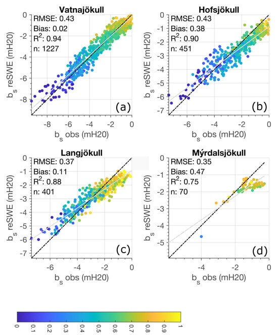
Figure 3.
Comparison of calculated and observed summer mass balance () for selected glaciers. (a) comparison for Vatnajökull, (b) comparison for Hofsjökull, (c) comparison for Langjökull and (d) comparison for Mýrdalsjökull. The dotted black line shows 1:1 and the gray line represents the calculated linear fit to the data. The color bar refers to the elevation of each observation point in the comparison with respect to the elevation range of each glacier, i.e., the normalized elevation range of each glacier.
4.3. Seasonal Snow
Figure 4a shows a comparison of time series from SWE calculated with the model and observations from a CS725 Snow Water Equivalent Sensor from 1 April each year (2015–2019) and until mid-July at Setur AWS. The general evolution of the SWE was represented by the model, especially during the active melt period, although discrepancies were observed, with overestimations of peak SWE in 2017 and 2018 and underestimation in 2015. In 2019 and 2016, the model reconstructs maximum SWE well. From 2016 to 2018, the timing and temporal evolution melt period were reconstructed well. In 2015 and 2019, the reconstructed SWE plateaus (∼120 DOY in 2019 and ∼185 DOY in 2015) and disconnects from the observed melt progress. The AWS at Setur is in a small flat area surrounded by small trenches, hills, and gullies where snow can accumulate, providing intermittent snow cover during the melt season. This difference could be explained by pixel classification as snow from MODIS data when snow has already melted at the AWS site. A time-lapse camera located at Setur partially confirms this behavior, and high-resolution imagery from Sentinel 2 and Landsat also shows the area with distributed snow patches in late spring. At Setur spatial variability of SWE has also been estimated on two 1 km long transects with a north–south and east–west orientation collected at 100 m intervals. The main snow pit and AWS observations were located at the midpoint of these two transects. For available observations at Setur, the standard deviation of snow depth was 0.3 m, with snow depths often observed as being more than twice as deep or shallow as at the snow pit location due to wind redistribution.
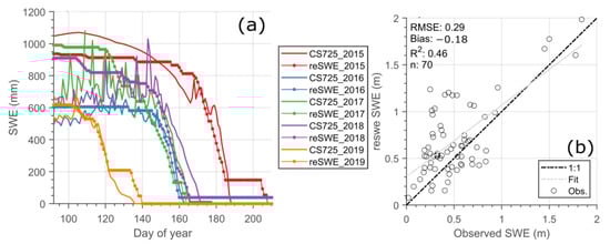
Figure 4.
(a) Comparison of SWE from 1 April 2015 to 2019 for observed SWE using a CS725 and estimation from the reconstructed SWE. (b) Comparison of observed maximum SWE in spring (mid-March to mid-April) against reconstructed SWE for selected years.
Figure 4b shows reconstructed maximum SWE from the model compared to all available snow pit observations. The comparison shows RMSE as 0.29 m, with a negative bias of 0.18 m. The comparison indicates that in some cases modeled data were overestimated, while fewer cases were underestimated. Observed SWE measurements represent snow depth and density well at the location of the observation, while many locations have limited representation of the near surroundings. Glacier mass balance components at Icelandic glaciers have better spatial representation from a point to their near surroundings as the observations were made in relatively flat areas.
5. Results
5.1. General Spatio-Temporal Characteristics of SWE
The annual SWE variability was generally high both for seasonal snow and glaciers. Figure 5 shows the spatial patterns for the average reconstructed SWE for seasonal snow and glacier ablation for the period 2000–2019. Two color maps were used to distinguish between glacier ablation (negative) and seasonal snow (positive). For seasonal snow, the largest SWE (>1000 mm) was found in mountainous and alpine areas close to the coast, notably in the East- and Westfjords, Tröllaskaga, and in the vicinity of glaciers. Smaller SWE was observed in the central highlands, flatter inland areas, and at lower elevations. This agrees with simulated precipitation climatologies by Crochet et al. [7], where less precipitation and dryer areas were found north of Vatnajökull and Hofsjökull and in the area between the two. It must be noted that in lower-elevation non-glaciated areas, the reconstruction might not represent accurately the total winter snowpack, as the buildup of a snowpack and complete melt-out in the period from October to March every year were frequent due to the high winter weather variability and melt-out events.
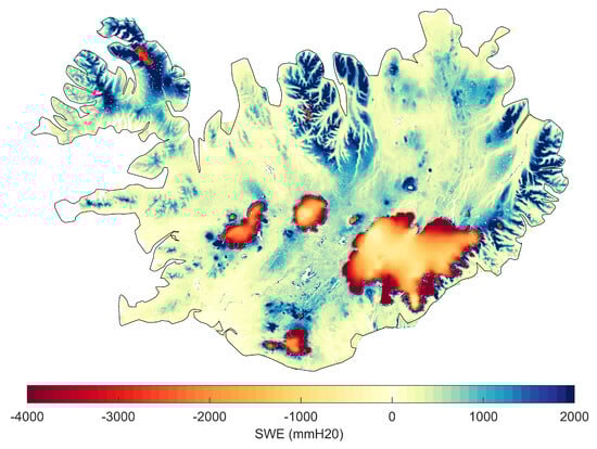
Figure 5.
Spatial pattern mean of reconstructed SWE and glacier ablation for the period 2000–2019. Glacier ablation is shown as negative values (white to red) and seasonal snow is shown as positive values(white to blue) to better distinguish seasonal snow and glacier ablation as their total magnitudes generally had different ranges.
For glaciers, more SWE (more ablation in ablation area) was generally associated with lower glacier elevations, while less ablation was observed at higher elevations (accumulation areas). For the dirty impurity-rich exposed bare ice areas, annually observed SWE was the highest, averaging more than 3000 mm, in agreement with surface mass balance observations [11,18,20]. Years with high summer ablation reveal certain patterns where more ablation was observed in the accumulation areas associated with cloud-free warm summer periods but also a strong link to below-average albedo due to light-absorbing particle (LAP) melt enhancements, reported in [44,57]. The lower limit of albedo (0.1 to 0.25) in the bare-ice areas further limits radiative forcing and reduces the annual melt variability in these areas, although melt-out timing of winter snow modulates melt variability and intensity [57].
Figure 6 shows the spatial distribution of the mean SWE for individual months from April to September for the period, i.e., mean accumulated average melt for each month. The gray areas indicate either snow-free areas or snow-covered areas where no melt is produced. In April and May, seasonal snow at lower and mid elevations was mostly depleted, with May generally producing more melt than April. The highest melt volumes were in May and June. In June and July, seasonal snow was mostly confined to high-SWE-accumulation areas. In September, and even August on a few occasions, small snowfalls were often observed, generally melted out; however, in some higher-elevation areas, these form the base for the following winter’s snowpack.
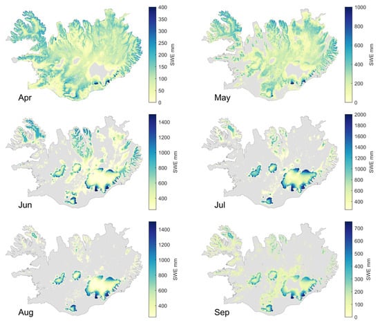
Figure 6.
Spatial patterns of mean reconstructed SWE for the period 2000–2019 for individual months from April to September. Note that the color scale is different for each figure.
For glaciers, melt onset was observed in April at lower elevations; for the low-elevation outlet glacier of southern Vatnajökull, melt was observed every month. With warmer temperatures and increasing short-wave energy in May and June, more glacier ablation was observed, generally peaking in late June to mid-July. As winter snow melted out, impurity-rich bare-ice areas were exposed, with low albedo values forcing more short-wave energy, increasing melt.
5.2. Inter-Annual Variability of SWE
Figure 7 shows annual spatial patterns for melt season (AMJJAS) SWE anomalies for 2000–2019. Blue colors represent anomalies below the mean, i.e., lower melt season average SWE values, while red areas represent values above the mean, contributing more seasonal SWE. No clear correlation was found between seasonal snow and glacier ablation, i.e., melt anomalies were not associated with same-sign anomalies for glaciers, although certain patterns could be identified. In 2000, a large negative anomaly was observed for seasonal snow in the north and in Austfirðir at higher elevations in the fjords. In the mountains and fjords closer to the sea in Austfirðir, higher values of SWE were observed. In the area north of Mýrdalsjökull and at Strandir, a positive SWE anomaly was observed. For all glaciers, except for the northern outlets of Vatnajökull, neutral or negative anomalies were observed. At northwest Vatnajökull (Dyngjujökull), an isolated area of melt enhancement was observed, which is unlikely to be linked to the 2000 Hekla eruption but is presumed to be a combination of residual effects from the Gjálp eruption in 1996 and dust transported from the pro-glacial areas near the terminus [44].
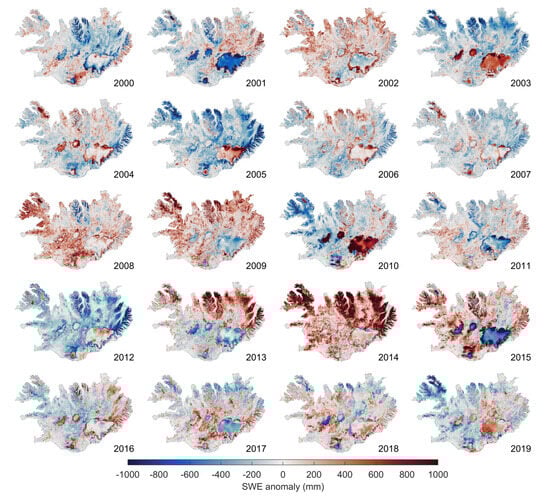
Figure 7.
Annual spatial patterns for SWE anomalies for 2000–2019. Red colors denote positive values where melt was above the average, i.e., more melt, while blue colors show less melt.
In 2001, 2009, 2011, 2013, 2015, and partially 2017 all main glaciated areas had negative glacier ablation anomalies while high-melt years were seen in 2003–2008, 2010, 2012, 2014, and 2019. For glaciers, melt-enhancing events can be defined as dust deposits from pro-glacial areas or other unstable erosive surfaces where the production of LAPs is often observed. Volcanic eruptions can also produce large amounts of ash and tephra that can deposit in glacier surfaces, influencing energy balance. The largest anomalies for glaciers were observed at all glaciers in 2010 associated with severe LAP deposition due to the volcanic eruption in Eyjafjallajökull during a warm and sunny summer. Less melt enhancement was observed associated with the 2011 Grímsvötn eruption at Vatnajökull, although the LAP deposits were quite clear in surface albedo data south and southeast of the Grímsvötn eruption site [44]. One difference between these two events for the southern outlet of Vatnajökull was the later onset of LAPs in 2011 but also a colder, cloudier spring and summer. In 2011, less incoming short-wave radiation was forced by the surface in June and much less was forced in July and August than in 2010, explaining most of the difference in melt. Had there been a similar climate in 2011 to that in 2010, much more melt could have been observed [57]. A positive melt anomaly in 2019 at all major glaciers except Drangajökull has been linked with extensive LAP deposits, with early melt-out of seasonal snow in the highlands exposing unstable dust hotspots, a rich source of LAPs transported by air.
Care must be taken when interpreting melt in areas where volcanic ash and tephra deposits influence melt, as the thickness of the deposit layer can have a great impact on the melt energy for actual melt. Generally, results show that a thin ash layer increases the snow and ice melt but an ash layer exceeding a certain critical thickness causes insulation. Dragosics et al. [68] reported that insulation effects of Icelandic dust and volcanic ash on snow and ice were observed at only 9–15 mm thickness depending on the type of material.
Schmidt et al. [69] performed simulations of the surface climate and energy balance of the Vatnajökull ice cap to estimate the glacier runoff sensitivity to the spring conditions, e.g., snow thickness. The simulations showed that runoff variability for the whole ice cap was on average 31% as a function of varying spring conditions, and higher for certain outlets (Brúarjökull, 50% of the variability). Snow thickness in the ablation area was a major control on the timing of the exposure of the underlying impurity-rich bare ice. From Figure 7, some years with high seasonal snow (red colors) and low glacier ablation (blue colors) can be identified. Years such as 2001, 2009, 2011, 2013, 2015, and 2017 exhibit a pattern where seasonal snow was above average in the highlands and glacier ablation was overall below average. Other years, such as 2003, 2005, 2010, 2012, and 2019, show the opposite: less seasonal snow and above-average glacier ablation. This supports the control and relationship between the impact of thick winter snow in the ablation area modulating melt due to delayed timing of impurity-rich bare ice exposure and vice versa. The accumulation of seasonal snow is driven by winter precipitation and temperature climatology and dominant storm tracks during the winter season, whereas glacier summer ablation is driven by spring and summer temperatures, cloud cover extent and persistence, and surface albedo, often impacted by LAPs. Because of this, no consistent annual relationship between seasonal snow and glacier ablation patterns was observed other than the suggested impact of winter snow thickness.
Figure 8 shows, in two panels, the accumulated maximum SWE in mm for the selected catchments and glaciers in Figure 1. The upper panels show basin-wide SWE for non-glaciated areas while the lower panel shows the basin-wide SWE for the glaciated part of the catchment. As seen in Figure 5, high seasonal snow areas where the largest average SWE (>1000 mm) was observed are Austfirðir, Tröllaskagi, Strandir, and Vestfirðir. Medium seasonal snow areas where SWE ranges from 600 to 1000 mm were observed are Lagarfljótsós, Skjálfandafljót, Markarfljót, Núpsvötn, and Gýgjukvísl. Other areas on average have small SWE (<500 mm).
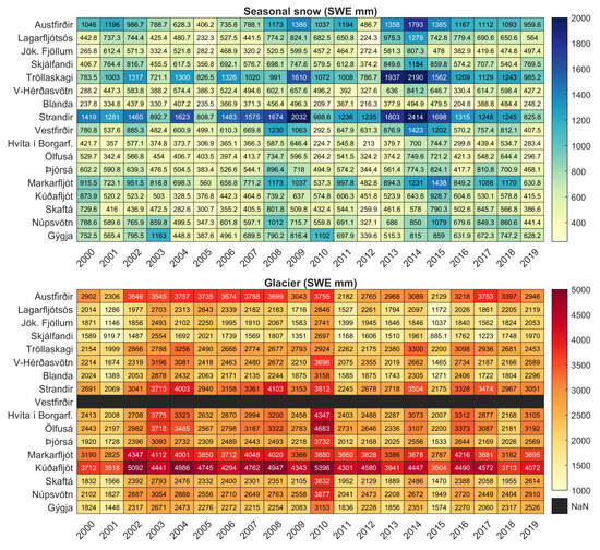
Figure 8.
Reconstructed SWE for the main catchments and individual years.
All areas show high variability, with certain groupings of years with similar conditions. Generally, below-average conditions were seen in 2001, 2003–2007, 2010, 2012, 2016, and 2019 for all the main catchments. The years 2005 and 2012 have the largest negative deviations, with SWE 130% below average values. Above-average conditions were seen in 2002, 2008–2009, 2014–2015, and 2017–2018. The highest SWE deviations were seen in 2014 and 2015 for all main catchments, with SWE on average 180% and 135% above average, respectively. Other years have less decisive patterns.
For the glaciated part of the main catchments, the highest SWE values (>3000 mm) were seen for glaciers in Austfirðir, Strandir, Markarfljót, and Kúðafljót, with average values above 4000 mm for Kúðafljót. Glacier ablation contributing to Markarfljót and Kúðafljót originates from the northern part of Mýrdalsjökull which has large areas of the glacier at relatively low elevations (220–300 m a.s.l.) and large unstable erosive surfaces that provide a constant source of LAPs [44]. The lowest SWE values (<2000 mm) were seen for Jökulsá á Fjöllum and Skjálfandafljót, as could be expected, as the glaciated parts of the catchment were distributed over quite high elevations, especially in the case of Skjálfandafljót ( 1040 m a.s.l.). Other glaciated main catchments show average SWE values between 2000 and 3000 mm.
Similar to seasonal snow melt, glacier ablation variability between years was quite high. Below-average conditions were seen in 2000, 2001, 2009, 2011–2013, and 2015, with 2001 and 2015 showing the largest deviations of 166% and 173% below the period-wide averages, respectively. Above-average conditions were seen in 2003–2008, 2010, 2014, and 2016 for nearly all catchments. In 2019, all glaciers had above-average conditions, with the exception of glaciers in Vestfirðir and Tröllaskagi. These glaciers were less influenced by conditions providing extensive amounts of LAPs deposited in the glacier surface enhancing melt [44]. Other years have less decisive patterns.
No significant correlation was observed between low SWE years for seasonal snow and above-average years for glacier ablation. For the period 2003–2007, generally below-average SWE values were observed for seasonal snow and above-average ablation was observed for glaciers. Similar conditions were seen in 2019, when the early country-wide melt-out of seasonal snow exposed erosive unstable pro-glacial surfaces and favorable weather conditions allowed for severe dust-depositing events.
Figure 9 shows the distribution of melt volume contribution for the main catchments, divided between SWE from seasonal snow and glacier ablation. The variability was smaller for areas with very high or low glacier ratios in the catchment. For Austfirðir, less than 5% of the annual melt water was contributed by glacier ablation, and less than 10–15% for Skjálfandi, Standir, and Töllaskagi and more than 90% of the melt water contribution was glacier-based for Gýgja, although 20% of the catchment area is non-glaciated. For Blanda and Hvíta í Borgarfirði, only about 8–9% of the catchment was glaciated but this part provides roughly 20–60% of the melt water volume. Jökulsá á Fjöllum, Kúðafljót, Lagarfljót, and Markarfljót og Skaftá have 15–20% of their catchment glaciated but receive glaciated ablation water volume ranging from 30 up to 75%.
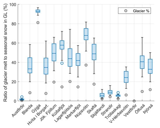
Figure 9.
Variability of ratio between melt contribution from seasonal snow and glacier ablation. Gray circles show the catchment area ratio between land and glacier. On each box, the central mark indicates the median, and the bottom and top edges of the box indicate the 25th and 75th percentiles, respectively. The whiskers extend to the most extreme data points not considered outliers. Outliers are shown as blue circles.
Figure 10 shows melt in mm (upper panel) and melt volume anomalies in percent (lower figure) for the main Icelandic glaciers and their sub-areas. A melt anomaly of 100% represents the mean for the period from 2000 to 2019, while the values below 100% represent below-average melt and vice versa. Glaciers and their sub-outlets are listed from the lowest average ablation (top) to the highest (bottom).
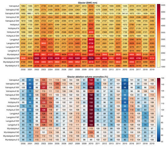
Figure 10.
Melt in mm (upper panel) and melt volume anomalies in percent (lower figure) for the main Icelandic glaciers and their sub-areas. A melt anomaly of 100% represents the mean for the period of 2000–2019 while values below 100% represent below-average melt and vice versa. Glaciers and their sub-outlets are listed from the lowest average melt (top) to the highest (bottom).
The highest ablation was observed for northeastern Mýrdalsjökull, closely followed by the other main outlets of Mýrdalsjökull. The northeastern outlet of Mýrdalsjökull is relatively flat, its elevation span being the lowest at Mýrdalsjökull. The glacier has close proximity to dust-producing erosive pro-glacial areas and warmer temperatures near the south coast of Iceland. Due to its proximity to the south coast, it receives large amounts of precipitation from frequently passing lows from the south and southwest storm tracks, with larger orographic uplift and precipitation than most other glaciers in Iceland [7,17]. Therefore, its high summer ablation is counterbalanced by high winter accumulation. Langjökull and Hofsjökull often had similar summer ablation magnitudes, while in most cases more ablation was observed at Langjökull, especially at the southern outlets. The largest glacier, Vatnajökull, had the lowest average summer ablation values. As with the southern outlets at Mýrdalsjökull, the southern outlets of Vatnajökull had higher ablation values than other outlets, especially in the north. This was driven by similar processes to those at Mýrdalsjökull: generally warmer temperatures, proximity to the coast, and frequently passing lows from the south and southwest storm tracks.
High annual variability was observed for all glaciers. Figure 10’s lower panel shows the melt volume anomalies from total annual melt volumes. As previously discussed, the high positive 2010 anomaly was driven by melt-enhancing LAPs from the eruption at Eyjafjallajökull and a persistent cloud-free summer with warm temperature, maximizing the impact of LAPs in the glacier surfaces. In the period from 2003 to 2008, melt volumes were generally above average, with the exception of Hofsjökull and Langjökull in 2005. Below-average glacier ablation was observed in 2000, 2001, 2013, 2015, and 2017–2018. The year 2015 was the first since the glaciological year of 1994/95 in which net mass balance was reported positive for glaciers with observed mass balance coincident with the lowest modeled glacier ablation in 2015 [11,18,20].
5.3. Melt Trends
Figure 11 shows the spatial pattern of the mean melt season (AMJJAS) trends in terms of the total change of a least-square fit to the SWE from 2000 to 2019. Statistically significant trends (p < 0.05) are shown with stipples. Negative significant trends at the terminus of glaciers were expected due to glacier retreat in recent decades, with associated debris deposits on dead ice [8]. No other significant negative trends were detected. At the northern outlet glaciers of Vatnajökull, Brúarjökull, and Dyngjujöklull, non-significant trends were observed concurrent with an increasing significant albedo trend for the same period [44]. These were in the end-of-year equilibrium-line altitude (ELA) area which varies from year to year. This pattern might support changes since 2012, when more winter bass balance has been observed and generally less summer ablation, pushing the ELA to lower elevations [11]. For seasonal snow, significant positive trends were observed for most of the mountain tops in Austfirðir and Tröllaskagi. These trends align with recent results for the same period from [47], reporting that the snow cover extent spanned a longer time, i.e., that snow cover was extending further into the spring and summer months. It is noted that only 20 years of data were available when reporting trends.
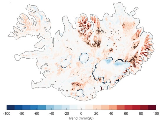
Figure 11.
Spatial pattern of mean melt season (AMJJAS) trends in terms of the total change of a least-square fit to the SWE from 2000–2019. Statistically significant trends (p < 0.05) are shown with stipples.
6. Conclusions
In this study, snow water equivalent was reconstructed using a gap-filled satellite-observed albedo and fractional snow cover data forced with climatological data. Data were calculated at a 500 m spatial resolution from 2000 until 2019 from mid-March out through September, spanning the spring and summer melt periods.
Energy balance components were thoroughly evaluated using in situ AWS data with good statistical agreement. For the reconstruction of glacier ablation, long-term extensive in situ data of mass balance observations were available to evaluate the results. Good statistical agreement was found between the model results and observations. For seasonal snow, much less in situ data were available to evaluate the model results, although the limited data available show acceptable performance.
Overall, the results show high annual variability in seasonal snow and glacier ablation SWE production. For seasonal snow, the majority of melt water production was observed in April and May, while high accumulation areas in the highlands retain snow into June and July. Glaciers had limited ablation in April, although high ablation values were observed close to the south coast. The majority of the ablation occurs in June, July, and August, with increasing bare ice exposure but decreasing solar elevation angles (less availability of short-wave energy), while May and September produce less ablation water on average.
Light-absorbing particles (LAPs) produced in volcanic eruptions and from pro-glacial hotspots deposited in the surfaces of glaciers have a strong influence on glacier ablation, clearly evident in 2010 and 2019. Significant positive trends in SWE were observed in mountainous north and east Iceland, while in other areas, glaciers show a non-significant trend, although trends with only 20 years of data should be reported with care.
The model pipeline developed can utilize alternative climatological forcing data and the previously adopted methods to produce spatio-temporal gap-filled albedo, and fractional snow cover data can be utilized with alternative satellite products, allowing the model framework to be adapted to future data sources. Although many complex hydrological and glaciological processes are simplified or omitted in the model, its main strength can be found in the real-time usability of remotely sensed albedo and fractional snow cover. As the past few years in Iceland have shown, real-time assessment of the impact of LAPs from volcanic eruptions or large-scale extensive dust deposit events can provide vital information for the operation and optimization of water resource usage.
Author Contributions
A.G. conceived and designed the study, performed the analyses, and prepared the manuscript. S.M.G. contributed to the study design, interpretation of the results, and writing of the manuscript. All authors have read and agreed to the published version of the manuscript.
Funding
This research received no external funding.
Data Availability Statement
Albedo, snow cover and reconstructed SWE data is available upon request. Weather station data is available upon request to Veðurstofa Íslands.
Acknowledgments
The authors would like to thank Sibylle von Löwis of Menar at the Icelandic Met Office for providing automatic land weather station data.
Conflicts of Interest
The authors declare no conflict of interest.
Appendix A. Automatic Weather Station Statistics
Table A1.
Summary of meteorological observations sites used for evaluation. ID refers to location of the site, L for non-glaciated areas and G for glaciated areas. The last three columns, N. T obs., N. SW obs., and N. LW obs. indicate the number of usable days for each variable at each site.
Table A1.
Summary of meteorological observations sites used for evaluation. ID refers to location of the site, L for non-glaciated areas and G for glaciated areas. The last three columns, N. T obs., N. SW obs., and N. LW obs. indicate the number of usable days for each variable at each site.
| Lat. | Lon. | Ele. | Site Name | ID | N. T obs. | N. SW obs. | N. LW obs. |
|---|---|---|---|---|---|---|---|
| 63.979 | 21.6556 | 530 | Bláfjöll úrk. | L | 3313 | ||
| 63.969 | 21.666 | 530 | Bláfjöll | L | 3617 | ||
| 63.983 | 21.649 | 530 | Bláfjallaskáli | L | 3359 | ||
| 64.033 | 21.366 | 380 | Hellisskarð | L | 3412 | ||
| 64.055 | 21.253 | 360 | Ölkelduháls | L | 3434 | ||
| 64.056 | 21.346 | 597 | Skarðsmýrarfjall | L | 2451 | ||
| 64.240 | 21.463 | 771 | Skálafell | L | 3286 | ||
| 64.490 | 21.762 | 480 | Skarðsheiði Miðf. | L | 1734 | ||
| 64.452 | 21.403 | 500.5 | Botnsheiði | L | 3264 | ||
| 65.604 | 23.990 | 350 | Patreksfjörður | L | 861 | ||
| 65.552 | 21.825 | 377 | Arnkatla | L | 1072 | ||
| 65.578 | 21.322 | 282 | Ennishöfði | L | 704 | ||
| 65.656 | 23.002 | 510 | Þingmannaheiði | L | 236 | ||
| 66.044 | 23.307 | 753 | Þverfjall | L | 3571 | ||
| 66.075 | 23.198 | 550 | Seljalandsdalur | L | 3410 | ||
| 66.068 | 23.210 | 283 | Seljalandsdalur | L | 2611 | ||
| 65.123 | 20.696 | 383 | Austurárdalsháls | L | 1558 | ||
| 65.062 | 18.838 | 785 | Sáta | L | 3476 | ||
| 65.222 | 20.056 | 509 | Grímstunguheiði | L | 1203 | ||
| 65.313 | 19.847 | 490 | Auðkúluheiði Fri. | L | 420 | ||
| 65.230 | 19.717 | 506 | Kolka | L | 3557 | 944 | 944 |
| 65.341 | 17.243 | 405 | Svartárkot | L | 2939 | ||
| 65.748 | 18.001 | 580 | Vaðlaheiði | L | 3593 | ||
| 65.787 | 17.003 | 390 | Gæsafjöll | L | 1624 | ||
| 65.891 | 17.228 | 350 | Sóleyjarflatamelar | L | 1640 | ||
| 65.856 | 17.201 | 390 | Rauðhálsar | L | 721 | ||
| 65.060 | 16.210 | 563 | Upptyppingar | L | 3447 | ||
| 65.265 | 14.032 | 400 | Seyðisfjörður Kb. | L | 2280 | ||
| 65.223 | 14.258 | 949 | Gagnheiði | L | 3461 | ||
| 65.619 | 16.976 | 282 | Mývatn | L | 3615 | 2171 | 0 |
| 65.629 | 16.837 | 347 | Bjarnarflag | L | 1503 | ||
| 65.642 | 16.128 | 390 | Grímsstaðir á Fjöllum | L | 1268 | ||
| 65.710 | 16.878 | 560 | Reykjahlíðarheiði | L | 376 | ||
| 65.694 | 16.774 | 455 | Krafla | L | 1436 | ||
| 65.911 | 16.976 | 311 | Þeistareykir | L | 2535 | ||
| 65.375 | 15.883 | 450 | Möðrudalur | L | 2786 | ||
| 64.828 | 16.089 | 748 | Brúaröræfi | L | 2339 | ||
| 64.816 | 15.322 | 750 | Innri Sauðá | L | 726 | 554 | 554 |
| 64.798 | 14.789 | 590 | Líkárvatn | L | 1285 | ||
| 64.728 | 16.111 | 845 | Brúarjökull B10 | L | 2365 | 2392 | 2392 |
| 64.928 | 15.777 | 639 | Kárahnjúkar | L | 3617 | 527 | 527 |
| 65.108 | 15.529 | 373 | Brú á Jökuldal | L | 3615 | ||
| 64.815 | 15.423 | 655 | Eyjabakkar | L | 3617 | ||
| 65.079 | 14.674 | 573 | Hallormsstaðaháls | L | 3617 | ||
| 65.036 | 14.571 | 300 | Þórudalur | L | 336 | ||
| 64.995 | 14.510 | 300 | Brúðardalur | L | 2024 | ||
| 65.000 | 14.462 | 500 | Þórdalsheiði | L | 2360 | ||
| 65.018 | 14.453 | 640 | Hallsteinsdalsvarp | L | 2111 | ||
| 65.043 | 14.162 | 281 | Ljósá í Reyðarfirði | L | 734 | ||
| 65.161 | 13.688 | 559 | Neskaupstaður | L | 2666 | ||
| 63.775 | 19.677 | 870 | Tindfjöll | L | 2199 | ||
| 64.098 | 18.614 | 675 | Lónakvísl | L | 3474 | ||
| 64.025 | 18.119 | 555 | Laufbali | L | 3310 | ||
| 64.199 | 19.030 | 555 | Vatnsfell I | L | 454 | ||
| 64.195 | 19.046 | 539 | Vatnsfell | L | 2666 | ||
| 64.395 | 18.504 | 647 | Veiðivatnahraun | L | 3608 | 0 | 0 |
| 64.317 | 18.217 | 726 | Jökulheimar | L | 3601 | 2528 | 888 |
| 64.680 | 19.282 | 925 | Kerlingarfjöll | L | 336 | ||
| 64.604 | 19.018 | 693 | Setur | L | 3602 | 512 | 512 |
| 64.581 | 18.598 | 620 | Þúfuver | L | 3617 | ||
| 64.571 | 18.111 | 819 | Hágöngur | L | 2773 | ||
| 64.866 | 19.562 | 641 | Hveravellir | L | 3193 | ||
| 64.933 | 17.983 | 820 | Sandbúðir | L | 3579 | ||
| 64.133 | 19.725 | 279 | Haf við Ísakot | L | 422 | ||
| 66.063 | 18.630 | 450 | Ólafsfjörður | L | 2211 | ||
| 66.168 | 23.268 | 500 | Bolungarvík | L | 2327 | ||
| 66.152 | 18.936 | 546 | Fífladalir | L | 497 | ||
| 66.153 | 18.937 | 600 | Fífladalir | L | 38 | ||
| 66.153 | 18.935 | 550 | Siglufjörður | L | 2126 | ||
| 64.503 | 17.234 | 1689 | Dyngjujökull | G | 484 | ||
| 64.538 | 15.597 | 1141 | Hoff | G | 1688 | 1774 | |
| 64.514 | 20.450 | 588 | L01 | G | 2246 | 2254 | 2254 |
| 64.302 | 17.153 | 1207 | Ske02 | G | 37 | 39 | 39 |
| 64.728 | 16.111 | 779 | B10 | G | 3224 | 3296 | 3215 |
| 64.575 | 16.328 | 1216 | B13 | G | 2043 | 2725 | 2338 |
| 64.402 | 16.681 | 1526 | B16 | G | 2575 | 2730 | 2569 |
| 64.417 | 17.319 | 1405 | Grímsvötn | G | 2687 | 791 | |
| 64.182 | 16.335 | 528 | Br04 | G | 597 | 600 | |
| 64.368 | 16.282 | 1242 | Br07 | G | 395 | 397 | |
| 64.325 | 18.117 | 771 | T01 | G | 483 | 567 | 567 |
| 64.336 | 17.976 | 1068 | T03 | G | 1943 | 2586 | 2094 |
| 64.404 | 17.608 | 1466 | T06 | G | 2538 | 2632 | 1691 |
| 64.639 | 17.522 | 1945 | Bard | G | 1509 | 898 | |
| 64.406 | 17.267 | 1724 | Grímsfjall | G | 2495 | 1324 | |
| 63.611 | 19.158 | 1345 | MyrA | G | 385 | 413 | |
| 64.594 | 20.374 | 1095 | L05 | G | 2536 | 2544 | 2544 |
| 64.770 | 18.543 | 840 | HNA09 | G | 292 | 307 | 307 |
| 64.813 | 18.648 | 1235 | HNA13 | G | 294 | 307 | 307 |
| 64.677 | 15.581 | 766 | E01 | G | 106 | 121 | 121 |
| 64.611 | 15.615 | 1190 | E03 | G | 115 | 122 | 122 |
References
- Rittger, K.; Bair, E.H.; Kahl, A.; Dozier, J. Spatial estimates of snow water equivalent from reconstruction. Adv. Water Resour. 2016, 94, 345–363. [Google Scholar] [CrossRef]
- Sandoval-Solis, S. Water Resources Management in California; Springer International Publishing: Cham, Switzerland, 2020; pp. 35–44. [Google Scholar] [CrossRef]
- Elder, K.; Dozier, J.; Michaelsen, J. Snow accumulation and distribution in an Alpine Watershed. Water Resour. Res. 1991, 27, 1541–1552. [Google Scholar] [CrossRef]
- Elder, K.; Rosenthal, W.; Davis, R.E. Estimating the spatial distribution of snow water equivalence in a montane watershed. Hydrol. Process. 1998, 12, 1793–1808. [Google Scholar] [CrossRef]
- Einarsson, M.A. Climates of the Oceans, H. Van Loon (Ed.). Vol. 15 of World Survey of Climatology, Editor-in-Chief H. E. Landsberg. J. Climatol. 1984, 5, 673–697. [Google Scholar] [CrossRef]
- Perkins, H.; Hopkins, T.S.; Malmberg, S.A.; Poulain, P.M.; Warn-Varnas, A. Oceanographic conditions east of Iceland. J. Geophys. Res. Ocean. 1998, 103, 21531–21542. [Google Scholar] [CrossRef]
- Crochet, P.; Jóhannesson, T.; Jónsson, T.; Sigurðsson, O.; Björnsson, H.; Pálsson, F.; Barstad, I. Estimating the Spatial Distribution of Precipitation in Iceland Using a Linear Model of Orographic Precipitation. J. Hydrometeorol. 2007, 8, 1285–1306. [Google Scholar] [CrossRef]
- Hannesdóttir, H.; Sigurðsson, O.; Þrastarson, R.H.; Guðmundsson, S.; Belart, J.M.; Pálsson, F.; Magnússon, E.; Víkingsson, S.; Kaldal, I.; Jóhannesson, T. A national glacier inventory and variations in glacier extent in Iceland from the Little Ice Age maximum to 2019. Jökull 2020, 12, 1–34. [Google Scholar] [CrossRef]
- Hjaltason, S.; Guðmundsdóttir, M.; Haukdal, J.Á.; Guðmundsson, J.R. Energy Statistics in Iceland 2019; Technical Report; Orkustofnun: Reykjavík, Iceland, 2020. [Google Scholar]
- Jóhannesson, T.; Aðalgeirsdóttir, G.; Björnsson, H.; Crochet, P.; Elíasson, E.B.; Guðmundsson, S.; Jónsdóttir, J.; Ólafsson, H.; Pálsson, F.; Rögnvaldsson, Ó.; et al. Effect of Climate Change on Hydrology and Hydro-Resources in Iceland; Orkustofnun: Reykjavík, Iceland, 2007. [Google Scholar]
- Pálsson, F.; Gunnarsson, A.; Jónsson, G.; Pálsson, H.S.; Steinþórsson, S. Vatnajökull: Mass Balance, Meltwater Drainage and Surface Velocity of the Glacial Year 2018–2019; LV-2020-016; Landsvirkjun: Reykjavík, Iceland, 2020; pp. 1–56. [Google Scholar]
- Björnsson, H.; Sigurðsson, B.D.; Davíðsdóttir, B.; Ólafsson, J.S.; Ástþórsson, Ó.S.; Ólafsdóttir, S.; Baldursson, T.; Jónsson, T. Loftslagsbreytingar og áhrif þeirra á Íslandi: Skýrsla Vísindanefndar um Loftslagsbreytingar 2018; Veðurstofa Íslands: Reykjavík, Iceland, 2018; pp. 1–238. [Google Scholar]
- Schmidt, L.S.; Ađalgeirsdóttir, G.; Pálsson, F.; Langen, P.L.; Guđmundsson, S.; Björnsson, H. Dynamic simulations of Vatnajökull ice cap from 1980 to 2300. J. Glaciol. 2020, 66, 97–112. [Google Scholar] [CrossRef]
- Milly, P.C.D.; Betancourt, J.; Falkenmark, M.; Hirsch, R.M.; Kundzewicz, Z.W.; Lettenmaier, D.P.; Stouffer, R.J. Stationarity Is Dead: Whither Water Management? Science 2008, 319, 573. [Google Scholar] [CrossRef]
- Björnsson, H.; Thorsteinsson, T. Climate Change and Energy Systems: Impacts, Risks and Adaptation in the Nordic and Baltic Countries; TemaNord, Nordic Council of Ministers: Copenhagen, Denmark, 2012. [Google Scholar] [CrossRef]
- Sveinsson, Ó. Energy in Iceland: Adaptation to Climate Change; UNU-FLORES Policy Briefs, United Nations University Institute for Integrated Management of Material Fluxes and of Resources (UNU-FLORES): Dresden, Germany, 2016. [Google Scholar]
- Ágústsson, H.; Hannesdóttir, H.; Thorsteinsson, T.; Pálsson, F.; Oddsson, B. Mass balance of Mýrdalsjökull ice cap accumulation area and comparison of observed winter balance with simulated precipitation. Jökull 2013, 63, 91–104. [Google Scholar] [CrossRef]
- Þorsteinsson, Þ.; Jóhannesson, T.; Sigurðsson, O.; Einarsson, B. Afkomumælingar á Hofsjökli 1988–2017; 2017-016; Veðurstofa Íslands: Reykjavík, Iceland, 2017; pp. 1–82. [Google Scholar]
- Pálsson, F.; Gunnarsson, A.; Pálsson, H.S.; Steinþórsson, S. Vatnajökull: Mass Balance, Meltwater Drainage and Surface Velocity of the Glacial Year 2020–2021; LV-2022-09; Landsvirkjun: Reykjavík, Iceland, 2022; pp. 1–62. [Google Scholar]
- Pálsson, F.; Gunnarsson, A.; Pálsson, H.S.; Steinþórsson, S. Afkomu- og Hraðamælingar á Langjökli Jökulárið 2018–2019; LV-2020-017; Landsvirkjun: Reykjavík, Iceland, 2020. [Google Scholar]
- Jónsson, T. Langtímasveiflur I, Snjóhula og Snjókoma; Greinargerð 02035; Veðurstofa Íslands: Reykjavík, Iceland, 2002; pp. 1–25. [Google Scholar]
- Jónsson, T.; Jónasson, K. Fimmtíu ára Snjódýpt á Íslandi; Greinargerð VÍ-G97025-ÚR20; Veðurstofa Íslands: Reykjavík, Iceland, 1997; pp. 1–25. [Google Scholar]
- Jóhannesson, T.; Sigurðsson, O. Samantekt um Snjómælingar á Hálendi Íslands; 2014-01; Veðurstofa Íslands: Reykjavík, Iceland, 2014; pp. 1–21. [Google Scholar]
- Sigurðsson, F.H.; Pálsdóttir, T.; Antonsson, T.K. Veðurstöð og Veðurfar á Hveravöllum á Kili; Rit Veðurstofu Íslands 20; Veðurstofa Íslands: Reykjavík, Iceland, 2003. [Google Scholar]
- Rist, S. Snjómæling Inni á Hálendinu Úrkomumælingar; Skilagrein 164; Vatnamælingar, Raforkumálastjóri: Reykjavík, Iceland, 1958; pp. 1–9. [Google Scholar]
- Rist, S. Snjómælingar vetur 1965/1966; Skilagrein 292; Vatnamælingar, Raforkumálastjóri: Reykjavík, Iceland, 1966; p. 1. [Google Scholar]
- Rist, S. Afstæð Snjódýptarmæling á Hálendinu; SR-81/03; Orkustofnun: Reykjavík, Iceland, 1981; pp. 1–4. [Google Scholar]
- Sigurðsson, O. Fyrirkomulag Snjómælinga á Hálendi Íslands; Greinargerð OSig-2002/03; Orkustofnun: Reykjavík, Iceland, 2002; pp. 1–3. [Google Scholar]
- Martinec, J.; Rango, A. Areal distribution of snow water equivalent evaluated by snow cover monitoring. Water Resour. Res. 1981, 17, 1480–1488. [Google Scholar] [CrossRef]
- Raleigh, M.S.; Lundquist, J.D. Comparing and combining SWE estimates from the SNOW-17 model using PRISM and SWE reconstruction. Water Resour. Res. 2012, 48, W01506. [Google Scholar] [CrossRef]
- Lettenmaier, D.P.; Alsdorf, D.; Dozier, J.; Huffman, G.J.; Pan, M.; Wood, E.F. Inroads of remote sensing into hydrologic science during the WRR era. Water Resour. Res. 2015, 51, 7309–7342. [Google Scholar] [CrossRef]
- Bair, E.H.; Abreu Calfa, A.; Rittger, K.; Dozier, J. Using machine learning for real-time estimates of snow water equivalent in the watersheds of Afghanistan. Cryosphere 2018, 12, 1579–1594. [Google Scholar] [CrossRef]
- Adam, J.C.; Lettenmaier, D.P. Adjustment of global gridded precipitation for systematic bias. J. Geophys. Res. Atmos. 2003, 108. [Google Scholar] [CrossRef]
- Adam, J.C.; Clark, E.A.; Lettenmaier, D.P.; Wood, E.F. Correction of Global Precipitation Products for Orographic Effects. J. Clim. 2006, 19, 15–38. [Google Scholar] [CrossRef]
- Cline, D.W.; Bales, R.C.; Dozier, J. Estimating the spatial distribution of snow in mountain basins using remote sensing and energy balance modeling. Water Resour. Res. 1998, 34, 1275–1285. [Google Scholar] [CrossRef]
- Molotch, N.P.; Painter, T.H.; Bales, R.C.; Dozier, J. Incorporating remotely-sensed snow albedo into a spatially-distributed snowmelt model. Geophys. Res. Lett. 2004, 31, L03501. [Google Scholar] [CrossRef]
- Painter, T.H.; Rittger, K.; McKenzie, C.; Slaughter, P.; Davis, R.E.; Dozier, J. Retrieval of subpixel snow covered area, grain size, and albedo from MODIS. Remote Sens. Environ. 2009, 113, 868–879. [Google Scholar] [CrossRef]
- Schneider, D.; Molotch, N.P. Real-time estimation of snow water equivalent in the Upper Colorado River Basin using MODIS-based SWE Reconstructions and SNOTEL data. Water Resour. Res. 2016, 52, 7892–7910. [Google Scholar] [CrossRef]
- Magnússon, E.; Belart, J.M.; Pálsson, F.; Anderson, L.S.; Gunnlaugsson, Á.Þ.; Berthier, E.; Ágústsson, H.; Geirsdóttir, Á. The subglacial topography of Drangajökull ice cap, NW-Iceland, deduced from dense RES-profiling. Jökull 2016, 66, 1–26. [Google Scholar] [CrossRef]
- Björnsson, H. Hydrology of Ice Caps in Volcanic Regions; Reykjavík Vísindafélag Íslendinga: Reykjavík, Iceland, 1988. [Google Scholar]
- Björnsson, H.; Pálsson, F.; Guðmundsson, M.T. Surface and bedrock topography of the Mýrdalsjökull ice cap, Iceland: The Katla caldera, eruption sites and routes of jökulhlaups. Jökull 2000, 49, 29–46. [Google Scholar] [CrossRef]
- Pálsson, F.; Guðmundsson, S.; Björnsson, H. Afkomu- Og Hraðamælingar á Langjökli Jökulárið 2011–2012; Technical Report LV-2015-076; Institute Earth Science, Univeristy Iceland and Landsvirkjun: Reykjavík, Iceland, 2013. [Google Scholar]
- Pálsson, F.; Gunnarsson, A.; Jónsson, G.; Pálsson, H.S.; Steinþórsson, S. Vatnajökull: Mass Balance, Meltwater Drainage and Surface Velocity of the Glacial Year 2014–2015; LV-2016-031; Landsvirkjun: Reykjavík, Iceland, 2016; pp. 1–64. [Google Scholar]
- Gunnarsson, A.; Gardarsson, S.M.; Pálsson, F.; Jóhannesson, T.; Sveinsson, O.G.B. Annual and inter-annual variability and trends of albedo of Icelandic glaciers. Cryosphere 2021, 15, 547–570. [Google Scholar] [CrossRef]
- Van den Broeke, M.; Reijmer, C.H.; Van De Wal, R.S. A study of the surface mass balance in Dronning Maud Land, Antarctica, using automatic weather stations. J. Glaciol. 2004, 50, 565–582. [Google Scholar] [CrossRef]
- Van den Broeke, M.; van As, D.; Reijmer, C.; Wal, R. Assessing and Improving the Quality of Unattended Radiation Observations in Antarctica. J. Atmos. Ocean. Technol. 2004, 21. [Google Scholar] [CrossRef]
- Gunnarsson, A.; Pálsson, F.; Aðalgeirsdóttir, G.; Björnsson, H.; Guðmundsson, S. Monitoring Energy Balance of Icelandic Glaciers for 25 years. In Proceedings of the 27th IUGG General Assembly, Montréal, QC, Canada, 8–18 July 2019. IUGG19-3435. [Google Scholar]
- Wang, L.; Qu, J.J.; Xiong, X.; Hao, X.; Xie, Y.; Che, N. A new method for retrieving band 6 of aqua MODIS. IEEE Geosci. Remote Sens. Lett. 2006, 3, 267–270. [Google Scholar] [CrossRef]
- Berrisford, P.; Dee, D.; Poli, P.; Brugge, R.; Fielding, M.; Fuentes, M.; Kållberg, P.; Kobayashi, S.; Uppala, S.; Simmons, A. The ERA-Interim Archive Version 2.0; ECMWF: Reading, UK, 2011; Volume 23. [Google Scholar]
- Rögnvaldsson, Ó.A. RÁVII: Tæknileg útfærsla á Niðurkvörðun á Íslandsveðri; Technical Repor; Belgingur-Reiknistofa í Veðurfræði: Reukjavik, Iceland, 2016. [Google Scholar]
- Crochet, P.; Jóhannesson, T. A data set of gridded daily temperature in Iceland, 1949–2010. Jökull 2011, 61, 1–17. [Google Scholar] [CrossRef]
- Nawri, N.; Björnsson, H.; Petersen, G.N.; Jónasson, K. Empirical Terrain Models for Surface Wind and Air Temperature over Iceland, VÍ, 2012-009; Veðurstofa Íslands: Reykjavík, Iceland, 2012. [Google Scholar]
- Gardner, A.S.; Sharp, M.J.; Koerner, R.M.; Labine, C.; Boon, S.; Marshall, S.J.; Burgess, D.O.; Lewis, D. Near-Surface Temperature Lapse Rates over Arctic Glaciers and Their Implications for Temperature Downscaling. J. Clim. 2009, 22, 4281–4298. [Google Scholar] [CrossRef]
- Hodgkins, R.; Carr, S.; Pálsson, F.; Guðmundsson, S.; Björnsson, H. Modelling variable glacier lapse rates using ERA-Interim reanalysis climatology: An evaluation at Vestari- Hagafellsjökull, Langjökull, Iceland. Int. J. Climatol. 2013, 33, 410–421. [Google Scholar] [CrossRef]
- Plüss, C.; Ohmura, A. Longwave Radiation on Snow-Covered Mountainous Surfaces. J. Appl. Meteorol. 1997, 36, 818–824. [Google Scholar] [CrossRef]
- Ohmura, A. Physical Basis for the Temperature-Based Melt-Index Method. J. Appl. Meteorol. 2001, 40, 753–761. [Google Scholar] [CrossRef]
- Gunnarsson, A.; Gardarsson, S.M.; Pálsson, F. Modeling of surface energy balance for Icelandic glaciers using remote sensing albedo. EGUsphere 2022, 2022, 1–43. [Google Scholar] [CrossRef]
- Brubaker, K.; Rango, A.; Kustas, W. Incorporating radiation inputs into the snowmelt runoff model. Hydrol. Process. 1996, 10, 1329–1343. [Google Scholar] [CrossRef]
- Dozier, J.; Warren, S.G. Effect of viewing angle on the infrared brightness temperature of snow. Water Resour. Res. 1982, 18, 1424–1434. [Google Scholar] [CrossRef]
- Jepsen, S.M.; Molotch, N.P.; Williams, M.W.; Rittger, K.E.; Sickman, J.O. Interannual variability of snowmelt in the Sierra Nevada and Rocky Mountains, United States: Examples from two alpine watersheds. Water Resour. Res. 2012, 48, W02529. [Google Scholar] [CrossRef]
- Guan, B.; Molotch, N.P.; Waliser, D.E.; Jepsen, S.M.; Painter, T.H.; Dozier, J. Snow water equivalent in the Sierra Nevada: Blending snow sensor observations with snowmelt model simulations. Water Resour. Res. 2013, 49, 5029–5046. [Google Scholar] [CrossRef]
- Bair, E.H.; Rittger, K.; Davis, R.E.; Painter, T.H.; Dozier, J. Validating reconstruction of snow water equivalent in California’s Sierra Nevada using measurements from the NASA Airborne Snow Observatory. Water Resour. Res. 2016, 52, 8437–8460. [Google Scholar] [CrossRef]
- Huai, B.; van den Broeke, M.R.; Reijmer, C.H. Long-term surface energy balance of the western Greenland Ice Sheet and the role of large-scale circulation variability. Cryosphere 2020, 14, 4181–4199. [Google Scholar] [CrossRef]
- Raleigh, M.S.; Landry, C.C.; Hayashi, M.; Quinton, W.L.; Lundquist, J.D. Approximating snow surface temperature from standard temperature and humidity data: New possibilities for snow model and remote sensing evaluation. Water Resour. Res. 2013, 49, 8053–8069. [Google Scholar] [CrossRef]
- Cogley, J.; Arendt, A.; Bauder, A.; Braithwaite, R.; Hock, R.; Jansson, P.; Kaser, G.; Moller, M.; Nicholson, L.; Rasmussen, L.; et al. Glossary of Glacier Mass Balance and Related Terms; Vol. 86, IHP-VII Technical Documents in Hydrology; International Hydrological Programme: Paris, France, 2010. [Google Scholar]
- Jennings, K.S.; Kittel, T.G.F.; Molotch, N.P. Observations and simulations of the seasonal evolution of snowpack cold content and its relation to snowmelt and the snowpack energy budget. Cryosphere 2018, 12, 1595–1614. [Google Scholar] [CrossRef]
- Schmidt, L.S.; Aðalgeirsdóttir, G.; Guðmundsson, S.; Langen, P.L.; Pálsson, F.; Mottram, R.; Gascoin, S.; Björnsson, H. The importance of accurate glacier albedo for estimates of surface mass balance on Vatnajökull: Evaluating the surface energy budget in a regional climate model with automatic weather station observations. Cryosphere 2017, 11, 1665–1684. [Google Scholar] [CrossRef]
- Dragosics, M.; Meinander, O.; Jónsdóttír, T.; Dürig, T.; De Leeuw, G.; Pálsson, F.; Dagsson-Waldhauserová, P.; Thorsteinsson, T. Insulation effects of Icelandic dust and volcanic ash on snow and ice. Arab. J. Geosci. 2016, 9, 126. [Google Scholar] [CrossRef]
- Schmidt, L.S.; Langen, P.L.; Aðalgeirsdóttir, G.; Pálsson, F.; Guðmundsson, S.; Gunnarsson, A. Sensitivity of Glacier Runoff to Winter Snow Thickness Investigated for Vatnajökull Ice Cap, Iceland, Using Numerical Models and Observations. Atmosphere 2018, 9, 450. [Google Scholar] [CrossRef]
Disclaimer/Publisher’s Note: The statements, opinions and data contained in all publications are solely those of the individual author(s) and contributor(s) and not of MDPI and/or the editor(s). MDPI and/or the editor(s) disclaim responsibility for any injury to people or property resulting from any ideas, methods, instructions or products referred to in the content. |
© 2023 by the authors. Licensee MDPI, Basel, Switzerland. This article is an open access article distributed under the terms and conditions of the Creative Commons Attribution (CC BY) license (https://creativecommons.org/licenses/by/4.0/).