Modeling Hydrodynamic Behavior of the Ottawa River: Harnessing the Power of Numerical Simulation and Machine Learning for Enhanced Predictability

Abstract

The Ottawa River Watershed is a vast area that stretches across Ontario and Quebec and holds great importance for Canada’s people, economy, and collective history, both in the present and the future. The river has faced numerous floods in recent years due to climate change. The most significant flood occurred in 2019, surpassing a 100-year flood event, and serves as a stark reminder of how climate change impacts our environment. Considering the limitations of machine learning (ML) models, which heavily rely on historical data used during training, they may struggle to accurately predict such “non-experienced” or “unseen” floods that were not encountered during the training process. To tackle this challenge, our study has utilized a combination of numerical modeling and ML to create an integrated methodology. Indeed, a comprehensive dataset of river flow discharge was generated using a numerical model, encompassing a wide range of potential future floods. This significantly improved the ML training process to generalize the accuracy of results. Utilizing this dataset, a novel ML model called the Expanded Framework of Group Method of Data Handling (EFGMDH) has been developed. Its purpose is to provide decision-makers with explicit equations for estimating three crucial hydrodynamic characteristics of the Ottawa River: floodplain width, flow velocity, and river flow depth. These predictions rely on various inputs, including the location of the desired cross-section, river slope, Manning roughness coefficient at different river sections (right, left, and middle), and river flow discharge. To establish practical models for each of the aforementioned hydrodynamic characteristics of the Ottawa River, different input combinations were tested to identify the most optimal ones. The EFGMDH model demonstrated high accuracy throughout the training and testing stages, achieving an R² value exceeding 0.99. The proposed model’s exceptional performance demonstrates its reliability and practical applications for the study area.

1. Introduction

The Ottawa River is a significant river that runs through Ontario and Quebec in eastern Canada. It is part of the St. Lawrence Basin and is the largest tributary to the St. Lawrence River. The Ottawa River plays a crucial role in the region’s hydrological cycle, acting as a primary drainage basin for an extensive watershed. The river collects and transports significant volumes of water, runoff, and sediment from its vast catchment area, influencing local and regional hydrological patterns [1]. The Ottawa River and its surrounding areas have experienced significant flooding events throughout history. In 2017, heavy rainfall and snowmelt led to extensive flooding in communities along the river, including Gatineau and Ottawa, reaching levels not seen in over 50 years [2]. It caused insured damages exceeding 220 million CAD [3], deemed as the century’s flood. During the spring of 2019, the Ottawa River encountered a flood that broke the previous record set just two years before. This caused the evacuation of thousands of people, extended states of emergency, and approximately 200 million CAD in insured losses [4]. This flood was exceptionally severe, with a discharge of 5980 m³/s, surpassing the expected level for a 100-year flood. Flooding in the Ottawa River region can occur due to a combination of factors, including heavy rainfall, rapid snowmelt, ice jams, and spring thaws [5]. The river’s large drainage basin and the potential for high water levels in its tributaries can exacerbate the risk of flooding [6]. According to climate change projections, there may be an increase in extreme weather events, such as heavy rainfall and precipitation, which could result in more frequent occurrences of flood-producing rainfall [4,7,8,9]. This could potentially increase the risk of flooding in the Ottawa River region, emphasizing the importance of adaptive strategies and long-term planning [10]. Consequently, developing predictive models for estimating floodplain width, flow velocity, and river flow depth during different flood events is crucial to enhance our understanding of flood dynamics, facilitating flood risk assessment, and supporting effective flood management strategies.

An accurate calculation of hydrodynamic characteristics is fundamental for effective flood management strategies. Floodplain width, river flow depth, and flow velocity are key factors that provide critical insights into the behavior and extent of flooding events. By quantifying the floodplain width, decision-makers can assess the potential impact on surrounding areas and identify at-risk zones. The measurement of floodplain width is vital in understanding the scale and impact of a flood event. It helps assess the potential inundation area, determines flood risk zones [11,12], and plans flood mitigation and management strategies [13]. River flow depth is a vital parameter for assessing the volume of water present and determining its potential to cause damage. The importance of river depth concerning floods can be understood through the following points: (i) Flood risk assessment [14,15]: Constitutes a cornerstone of disaster management and urban planning. Accurate estimates of river depth play a pivotal role in predicting the potential extent and severity of flooding. Researchers and policymakers can formulate effective strategies to mitigate flood-related risks, allocate resources, and prioritize vulnerable areas for intervention by analyzing historical flood data alongside river depth information. (ii) Hydraulic capacity: Understanding river depth is central to evaluating a watercourse’s hydraulic capacity, which refers to the volume of water a river channel can safely convey. Inadequate river depth can lead to increased flow velocities and, subsequently, heightened flood risks. By quantifying river depth, engineers and hydrologists can optimize hydraulic designs to ensure that rivers maintain their conveyance abilities even during high-flow events. (iii) Floodplain mapping [16]: Accurate floodplain mapping is indispensable for delineating areas susceptible to inundation during flood events. River depth data serves as a fundamental input for modeling floodplain extents. Detailed floodplain maps aid in land-use planning, infrastructure development, and emergency response coordination. Moreover, they empower communities to make informed decisions regarding building construction and resource allocation in flood-prone regions. (iv) Infrastructure design [17]: River depth information guides the design and construction of infrastructure, safeguarding against flood-related damage and disruption [16]. Bridges, culverts, and embankments must be engineered to withstand varying water levels. Inaccurate river depth estimations can compromise these assets’ structural integrity, leading to catastrophic failures during flood events. A precise understanding of river depth ensures resilient infrastructure that can endure the challenges posed by changing hydrological conditions. (v) Emergency response planning: Rapid and coordinated emergency response is essential to minimize loss of life and property damage during floods. Accurate river depth data enables authorities to anticipate the magnitude of potential flooding and allocate resources strategically. This facilitates the timely deployment of personnel, equipment, and supplies to the most vulnerable areas, enabling efficient rescue and relief efforts. Flow velocity measurements help understand the speed at which water moves, aiding in predicting flood progression and identifying areas prone to rapid inundation. The flow velocity during different floods is another crucial parameter with several vital implications. Here are some reasons why velocity is essential in understanding floods: (1) Flow dynamics [18]: The rate at which water moves within a river channel affects flood propagation and influences the interaction between water and its surroundings. Fluid mechanic principles dictate that varying flow velocities can lead to different flow patterns, such as laminar or turbulent flow, which in turn impact the behavior of floodwaters as they interact with structures, vegetation, and natural topography. (2) Flood hazard mapping [19]: Flow velocity helps determine the extent to which floodwaters can inundate a region, influencing floodplain delineation. This information is fundamental for identifying areas at risk, guiding land-use planning, and enabling emergency management agencies to develop targeted response strategies for regions vulnerable to swift-moving floodwaters. (3) Sediment Transport [20]: During flood events, fast-moving waters can transport sediments, debris, and pollutants downstream, potentially exacerbating flood impacts and altering river morphology. Understanding velocity patterns aids in predicting sediment deposition and erosion rates, facilitating informed decision-making for riverbed management and sediment control measures. (4) Hydraulic engineering design [21]: Structures such as bridges, culverts, and flood control channels need to be designed to withstand the forces exerted by flowing water. Accurate velocity estimations enable engineers to tailor structures to specific flow conditions, ensuring their stability and functionality even during extreme flood events. (5) Flood modeling and forecasting [22].

HEC-RAS (Hydrologic Engineering Centers-River Analysis System) has gained renown for its proficiency in scrutinizing and emulating river hydraulic processes. It has established itself as a well-recognized and extensively embraced software in the realm of hydraulic modeling, boasting a vast user community [23,24,25]. This software offers an array of capabilities for assessing and simulating river hydraulics, encompassing aspects such as floodplain deluge scenarios, sediment conveyance, water surface profiles, and flow rates [26,27,28,29]. It demonstrates its competence in accommodating diverse hydraulic conditions essential for the cartography of floodplains and handling intricate river systems, utilizing Geographic Information System data [30,31]. Nevertheless, it is worth noting that the computational demands of running simulations in HEC-RAS can vary based on the scale and intricacy of the model, sometimes necessitating substantial computational resources [32].

Machine Learning (ML) has gained widespread application in the prediction and analysis of time-varying cross-section rating curves [33,34] and hydrodynamic characteristics of rivers [35,36], efficiently processing and analyzing large data volumes, enabling accurate floodplain width, river depth, and flood flow velocity predictions [15,37,38]. Group Method of Data Handling (GMDH) [39] is a prominent and widely recognized ML technique [40,41,42,43]. The GMDH offers several advantages compared to the other ML techniques, including automatic feature selection [43], employing a self-organizing algorithm for optimizing the structure and complexity of the model [44], interpretability by providing simple and practical models [45], non-linearity handling [46], and adaptability [47]. These advantages make GMDH a valuable tool in various domains, particularly when dealing with complex datasets. Nevertheless, the GMDH has limitations, including the exclusion of non-adjacent layers, restriction to second-order polynomials, and a limitation to two neurons per layer. To overcome these drawbacks, the Expanded Framework of GMDH (EFGMDH) is introduced in the current study for forecasting the hydrodynamics characteristics of the river.

Although previous studies have demonstrated the high predictive capabilities of various ML algorithms in flood prediction, their accuracy heavily relies on the historical data used during the training process [48]. Acknowledging that none of these algorithms can anticipate “non-experienced” or “unseen” floods is essential. Given the impacts of climate change, significant changes in flood patterns have been observed in Canada. For instance, the 2019 flood surpassed the discharge levels expected once every 100 years, which caught decision-makers by surprise as such an event was unprecedented in historical records dating back to the 1900s.

To address these challenges, this study aims to combine numerical modeling with the ML approaches. A comprehensive dataset of river flow discharge will be generated using the numerical model (i.e., HEC-RAS), encompassing a wide range of potential future floods. This extensive dataset will serve as training input for ML algorithms, facilitating the development of user-friendly explicit equations for decision-makers. These equations will enable the direct calculation of three important hydrodynamic characteristics of the Ottawa River, including floodplain width, flow velocity, and river flow depth. By integrating numerical modeling and ML, this research enhances flood prediction accuracy and equips decision-makers with valuable tools for proactive flood management. This comprehensive approach acknowledges the evolving nature of flood patterns due to climate change. It provides a framework for anticipating and mitigating the impacts of future floods on the Ottawa River and its surrounding areas.

2. Materials and Methods

2.1. Study Area

The Ottawa River runs for approximately 1271 km (790 miles) from its source in Lake Capimitchigama in Quebec to its mouth at the confluence with the St. Lawrence River in Montreal, Quebec. The Ottawa River has a large drainage basin, covering an area of about 146,300 square kilometers, which extends its hydrological significance beyond its immediate vicinity. As it finally merges with the St. Lawrence River, providing approximately 80% of the water flow, it plays a crucial role in maintaining the water balance and ecosystem well-being of the broader watershed.

The study area was chosen upstream of the city of Ottawa to be able to analyze the impacts of high flows to protect the city. Then, the study area was selected in a stretch of river comprising at least two hydrometric stations to ensure reliable model calibration. Finally, the delimitation between the start and end of the zone is based on the region’s division of the Digital Elevation Model (DEM). Once this zone has been chosen, a division into sub-zones is carried out to share the river evenly. The zones are delimited according to the speed of flow, the width of the riverbed, and the nature of the banks. The geographical location of the study area and upstream and downstream boundaries of the study area are provided in Figure 1.

In the Ottawa River basin, during the period from October to April, temperatures remained lower than average, leading to frozen ground that was incapable of absorbing the moisture from the melting snow. However, most snow and ice did not begin the melting process until the middle of spring, resulting in certain forested regions experiencing snow accumulation exceeding the typical amount by 50%. From mid-April to mid-May, the area experienced a significant period of heavy rainfall, causing Ottawa to receive double its average precipitation with an accumulation of 150 mm. The combination of rain and melting snow overwhelmed the Ottawa River, surpassing its capacity. As a result, riverside communities in Ontario and Quebec were inundated by rising water levels.

Table 1. The descriptive statistics of the variables at the training and testing stages.

Parameter	Stage	Mean	SD	K	S	Min	Max
Slope	Train	0.358	0.352	2.199	1.760	0.05	1.27
	Test	0.361	0.353	2.212	1.757	0.05	1.27
nLeft	Train	0.0248	0.01053	−1.33	0.03	0.01	0.04
	Test	0.0249	0.01060	−1.35	0.04	0.01	0.04
nMiddle	Train	0.0247	0.010419	−1.293	0.040	0.01	0.04
	Test	0.0248	0.010504	−1.314	0.047	0.01	0.04
nRight	Train	0.0248	0.010516	−1.320	0.038	0.01	0.04
	Test	0.0249	0.010582	−1.335	0.047	0.01	0.04
Flow discharge (m3/s)	Train	4075.64	1489.824	−0.892	0.338	2000	7000
	Test	4135.29	1501.258	−0.872	0.361	2000	7000
River flow depth (m)	Train	3.11	0.649247	−0.179	0.376	1.87	5.22
	Test	3.14	0.658579	−0.222	0.402	1.83	4.93
Flow velocity (m/s)	Train	0.611	0.235912	1.310	1.225	0.29	1.52
	Test	0.613	0.240759	1.314	1.195	0.27	1.57
Floodplain width (m)	Train	1019.94	704.7546	0.798	1.279	131.8	2713
	Test	1021.67	692.4157	0.824	1.255	187.1	2713.4

SD = Standard Deviation; K = Kurtosis; S = Skewness; Min = Minimum; Max = Maximum.

provides the descriptive statistics of the variables at the training and testing stages. Based on the provided information in this table, it can be concluded that, on average, the magnitudes of all inputs (i.e., slope, n_Left, n_Middle, n_Right, and flow discharge) and outputs (i.e., river flow depth, flow velocity, and floodplain width) exhibit consistency at both stages. The n_Left, n_Middle, and n_Right are Manning’s roughness coefficients at the left, middle, and right sides of the channel, respectively, at each cross-section. In each zone, the slope of the riverbed was derived from the DEM. Furthermore, the standard deviations of these variables also indicate consistent variability in the measurements at both stages. Additionally, the sample variance values for all variables reflect comparable levels of dispersion in the measurements of all variables at both stages. The positive kurtosis values of the slope, flow velocity, and floodplain width at both training and testing stages suggest distributions with relatively heavier tails and more peaked shapes compared to a normal distribution. Conversely, the kurtosis values for the other parameters (i.e., n_Left, n_Middle, n_Right, flow discharge, and river flow depth) are negative, indicating distributions with relatively less peaked shapes and lighter tails than a normal distribution. Moreover, the positive skewness values indicate right-skewed distributions for all input and output variables, indicating longer tails on the right side.

2.2. Expanded Framework of GMDH (EFGMDH)

The Group Method of Data Handling (GMDH) (Ivakhnenko 1978) is a ML algorithm that belongs to the class of inductive modeling techniques, which has since been developed and applied in various fields [49,50]. GMDH, as a self-organizing ML technique [51], iteratively constructs interconnected polynomial models, starting with a simple model and progressively adding complexity in subsequent layers. The GMDH algorithm works by organizing the input variables into layers, where each layer represents a different level of complexity. The “number of layers” is a parameter the user defines before starting the model. The algorithm generates candidate models within each layer by combining different input variable subsets and evaluating their performance using various statistical criteria. The best-performing models from each layer are selected and become the input for the next layer. This process continues until a satisfactory model is obtained.

Let us assume h input variables and H observations for the purpose of estimating the target parameter (T) in the following manner [52]:

$$T=Q(x_{i1},x_{i2},\mathrm{\dots },x_{ih})\hspace{0.17em}\hspace{0.17em}\hspace{0.17em}\hspace{0.17em}\hspace{0.17em}\hspace{0.17em}\hspace{0.17em}\hspace{0.17em}\hspace{0.17em}\hspace{0.17em}\hspace{0.17em}\hspace{0.17em}\hspace{0.17em}\hspace{0.17em}(i=1,2,\mathrm{\dots },\mathrm{H})$$

(1)

Here, H represents the total number of observations or samples available, h signifies the number of input variables, Q() denotes the function establishing the relationship between the inputs, and T represents the actual target value.

The GMDH network has the ability to learn from diverse input systems, enabling it to effectively estimate the target variable through a distinct method [52], as shown below:

$$\widehat{T}=\widehat{Q}(x_{i1},x_{i2},\mathrm{\dots },x_{ih})\hspace{0.17em}\hspace{0.17em}\hspace{0.17em}\hspace{0.17em}\hspace{0.17em}\hspace{0.17em}\hspace{0.17em}\hspace{0.17em}\hspace{0.17em}\hspace{0.17em}\hspace{0.17em}\hspace{0.17em}\hspace{0.17em}\hspace{0.17em}(i=1,2,\mathrm{\dots },\mathrm{H})$$

(2)

Here, $\widehat{T}$ represents the approximated target value and $\widehat{Q}()$ represents the approximated function that maps the inputs to the target value. Indeed, the GMDH network is trained to find the best possible approximation of the target variable based on the given input system.

During the training phase, the primary challenge lies in determining and controlling the GMDH network to minimize the objective function. The objective function is defined as the squared difference between the approximated outputs generated via the GMDH network and the actual outputs. The goal is to find the network configuration that produces the closest approximation to the proper target, as shown below.

$$\underset{\mathit{min}}{{\displaystyle E_{GMDH}}}={\displaystyle \sum _{i=1}^H{\left(\widehat{T}-T_i\right)}^2}$$

(3)

In this context, T represents the actual output, $\widehat{T}$ represents the approximated output generated via the GMDH network, H represents the number of samples available for training and evaluation, and EGMDH represents the objective function of the GMDH model.

The Volterra series presents a compelling argument that establishes a fundamental formula for the network connection between the input and target parameters. It firmly supports the viewpoint that all systems can be effectively approximated by employing an infinite number of discrete series formulae [53]. Notably, the Kolmogorov–Gabor polynomial serves as a potent manifestation of the discrete form of the Volterra series, characterized by its definition as follows:

$$Q=P_0+{\displaystyle \sum _{m=1}^h{P}_m{x}_m+{\displaystyle \sum _{m=1}^h{\displaystyle \sum _{n=1}^h{P}_{mn}{x}_m{x}_n}}+{\displaystyle \sum _{m=1}^h{\displaystyle \sum _{n=1}^h{\displaystyle \sum _{o=1}^h{P}_{mno}{x}_m{x}_n{x}_o}}}}$$

(4)

In this context, {P₁, … P_h} represents a set of unknown parameters, where h denotes the number of input variables. On the other hand, {x₁, … x_h} represents the input variables themselves. The unknown parameters {P₁, … P_h}, determined via the training process, are crucial in defining the relationship between the input variables {x₁, … x_h} and the output variable.

An abridged representation of Equation (4), attained via the incorporation of second-order polynomials that exclusively engage two neurons, can be articulated as follows:

$$\widehat{Q}(x_m,x_n)=P_1+P_2{x}_m+P_3{x}_n+P_4{x}_m^2+P_5{x}_n^2+P_6{x}_m{x}_n$$

(5)

In the provided equation, x_m and x_n signify the inputs of the recently formed neurons, while P = {P₁, P₂, P₃, P₄, P₅, P₆} represents the collection of undisclosed parameters.

Within the conventional GMDH framework, the mathematical formula represented by Equation (5) is employed to establish a mapping between the neurons in the input layer, which correspond to the input variables and the output neuron located in the output layer. This mapping is achieved by utilizing newly produced neurons situated in the hidden layer(s). It is worth noting that all the created neurons, whether in the hidden layer(s) or the output layer, are generated using Equation (5). The distinction among the quadratic equations utilized to generate fresh neurons can be categorized into two primary aspects: (i) the computed values of the unidentified parameters P = {P₁, P₂, P₃, P₄, P₅, P₆}, and (ii) the nature of inputs (each neuron can be produced using solely two neurons).

The overall configuration of the network is established by amalgamating these quadratic polynomials alongside certain constraints, including the maximum allowable number of layers and the maximum permissible count of neurons in each layer. In the initial hidden layer, the GMDH algorithm employs a universal formula to compute the probability of two independent parameters derived from all input variables. By utilizing the neurons produced in the initial layer, the neurons in the subsequent layer are formed similarly. This iterative process persists until the maximum allowable number of layers is attained. The total number of feasible combinations achievable with two variables for k variables is A = R(R − 1)/2.

A matrix-based equation is formulated for each row of A by employing the second-order polynomial specified in Equation (5). This equation establishes the relationship between the variables and the corresponding row of A.

$$HP=Q$$

(6)

where

$$H=\left[\begin{array}{cccccc}1& x_{1m}& x_{1n}& x_{1m}{x}_{1n}& x_{1m}^2& x_{1n}^2\\ 1& x_{2m}& x_{2n}& x_{2m}{x}_{2n}& x_{2m}^2& x_{2n}^2\\ ⋮& ⋮& ⋮& ⋮& ⋮& ⋮\\ 1& x_{Am}& x_{An}& x_{Am}{x}_{An}& x_{Am}^2& x_{An}^2\end{array}\right]$$

(7)

$$P=\left[P_1,P_2,P_3,P_4,P_5,P_6\right]$$

(8)

$$Q={\left[Q_1,Q_2,\mathrm{\dots },Q_A\right]}^T$$

(9)

Equation (6) contains only one unknown variable, P, which is calculated in the following form:

$$P={\left(H^{T}H\right)}^{-1}{H}^{T}O$$

(10)

The classical GMDH methodology offers numerous advantages when compared to alternative ML techniques, including (i) provision of straightforward quadratic equations suitable for practical applications; (ii) self-organizing capability, allowing for the automatic design of the final model’s structure even in the absence of prior knowledge regarding the relationship between the target and corresponding input variables; (iii) each layer of the GMDH model contributes to prediction, enabling the removal of specific parameters without substantially impacting the overall outcome; (iv) the GMDH network carries a lower risk of overfitting, reducing the potential for the model to fit too closely to the training data [54]; and (v) the GMDH-based sorting algorithms exhibit a high degree of programmability, allowing for efficient customization and adaptation [49,55]. However, it is important to acknowledge the limitations of the conventional GMDH methodology, which include the following:

(1)

Polynomial structures (i.e., degree and number of inputs): The classical GMDH approach is limited to second-order polynomial structures with only two inputs.

(2)

Indirect connection with non-adjacent layers: In the classical GMDH, the generation of each new neuron in the nth layer is solely based on the existing neurons in the adjacent (n − 1)th layer.

(3)

Model complexity: In the classical GMDH, the complexity of the model is controlled by the user via the specification of the maximum number of neurons and layers prior to the modeling process. However, this approach does not guarantee the discovery of an optimal structure based solely on these two parameters and the objective function defined in Equation (3).

To address these limitations, the current study introduces the Expanded Framework of GMDH (EFGMDH) for the prediction of hydrodynamic characteristics in rivers. The EFGMDH framework aims to overcome the drawbacks associated with classical GMDH by offering enhanced capabilities and an improved modeling performance in the field of river forecasting. The proposed method incorporates the utilization of four distinct sets of polynomials to construct the final model structure: a second-order polynomial with two inputs (Equation (5)), a second-order polynomial with three inputs (Equation (11)), a third-order polynomial with two inputs (Equation (12)), and a third-order polynomial with three inputs (Equation (13)). The final structure of the model allows for the simultaneous combination of these polynomials. Additionally, the model facilitates the generation of new neurons from all neurons in the previous layers, including both neighboring and non-neighboring layers, as shown below.

$$\widehat{Q}(x_m,x_n,x_o)=P_1+P_2{x}_m+P_3{x}_n+P_4{x}_o+P_5{x}_m^2+P_6{x}_n^2+P_7{x}_o^2+P_8{x}_m{x}_n+P_9{x}_m{x}_o+P_{10}{x}_n{x}_o$$

(11)

$$\widehat{Q}(x_m,x_n)=P_1+P_2{x}_m+P_3{x}_n+P_4{x}_m^2+P_5{x}_n^2+P_6{x}_m{x}_n+P_7{x}_m{x}_n^2+P_8{x}_m^2{x}_n+P_9{x}_m^3+P_{10}{x}_n^3$$

(12)

$$\begin{array}{l}\widehat{Q}(x_m,x_n,x_o)=P_1+P_2{x}_m+P_3{x}_n+P_4{x}_3+P_5{x}_m^2+P_6{x}_n^2+P_7{x}_o^2\\ \hspace{0.17em}\hspace{0.17em}\hspace{0.17em}\hspace{0.17em}\hspace{0.17em}\hspace{0.17em}\hspace{0.17em}\hspace{0.17em}\hspace{0.17em}\hspace{0.17em}\hspace{0.17em}\hspace{0.17em}\hspace{0.17em}\hspace{0.17em}+P_8{x}_m{x}_n+P_9{x}_m{x}_o+P_{10}{x}_n{x}_o+P_{11}{x}_m^3+P_{12}{x}_n^3+P_{13}{x}_o^3+P_{14}{x}_m^2{x}_n\\ \hspace{0.17em}\hspace{0.17em}\hspace{0.17em}\hspace{0.17em}\hspace{0.17em}\hspace{0.17em}\hspace{0.17em}\hspace{0.17em}\hspace{0.17em}\hspace{0.17em}\hspace{0.17em}\hspace{0.17em}\hspace{0.17em}+P_{15}{x}_m^2{x}_o+P_{16}{x}_n^2{x}_m+P_{17}{x}_n^2{x}_o+P_{18}{x}_o^2{x}_m+P_{19}{x}_o^2{x}_n+P_{20}{x}_m{x}_n{x}_o\end{array}$$

(13)

Furthermore, the objective function employed in the EFGMDH model is the Akaike Information Criterion (AIC) [56]. The AIC provides a robust method for model selection by balancing goodness of fit and model complexity, allowing researchers to make informed decisions when choosing the most appropriate model for their data. AIC is based on information theory principles and follows the maximization of the likelihood function while penalizing for model complexity. The equation for the corrected version of the AIC (AICc), which has been utilized in recent hydrology studies [57,58,59], is provided as follows:

$$AICc=L\times Ln\left(\frac{1}{L}{\displaystyle \sum _{i=1}^L{\left(Q_{o,i}-Q_{m,i}\right)}^2}\right)+\frac{2KL}{L-K-1}$$

(14)

Here, the variables Q_o and Q_m represent the measured and estimated target variable, respectively. The total number of samples is denoted by L. The Ln is the natural logarithm. Additionally, the number of tuned parameters required to develop the final EFGMDH-based network (all polynomials in the final model) is represented by K. For second-order polynomials with two and three inputs (Equations (5) and (11)), the value of K is 6 and 10, respectively. On the other hand, for third-order polynomials (Equations (12) and (13)), K are (10) and (20) for polynomials with two and three inputs, respectively.

The AICc value is calculated for each model under consideration, and the model with the lowest AICc is typically chosen as the best-fitting model. Therefore, AICc allows for the comparison of models with different numbers of parameters, enabling the selection of a simpler model if it provides a comparable fit to a more complex one.

2.3. Reliability Analysis

Reliability analysis is a statistical technique used to assess the consistency, stability, and dependability of measurements, tests, or instruments. It aims to determine the extent to which a measurement or test produces consistent and reliable results over time or across different conditions. The reliability analysis (RA) [60] is defined as follows:

$$RA(\%)=\frac{100}{L}{\displaystyle {\sum }_{i=1}^L{Z}_i}$$

(15)

$$Z_i=\left\{\begin{array}{l}0\hspace{0.17em}\hspace{0.17em}\hspace{0.17em}\hspace{0.17em}\hspace{0.17em}\hspace{0.17em}\hspace{0.17em}\hspace{0.17em}\hspace{0.17em}\hspace{0.17em}\hspace{0.17em}\hspace{0.17em}\hspace{0.17em}\hspace{0.17em}\hspace{0.17em}\hspace{0.17em}\hspace{0.17em}\hspace{0.17em}\hspace{0.17em}\hspace{0.17em}\hspace{0.17em}\hspace{0.17em}\hspace{0.17em}\hspace{0.17em}\hspace{0.17em}\hspace{0.17em}\hspace{0.17em}{E}_i>\beta \\ 1\hspace{0.17em}\hspace{0.17em}\hspace{0.17em}\hspace{0.17em}\hspace{0.17em}\hspace{0.17em}\hspace{0.17em}\hspace{0.17em}\hspace{0.17em}\hspace{0.17em}\hspace{0.17em}\hspace{0.17em}\hspace{0.17em}\hspace{0.17em}\hspace{0.17em}\hspace{0.17em}\hspace{0.17em}\hspace{0.17em}\hspace{0.17em}\hspace{0.17em}\hspace{0.17em}\hspace{0.17em}\hspace{0.17em}\hspace{0.17em}\hspace{0.17em}\hspace{0.17em}\hspace{0.17em}\hspace{0.17em}{E}_i\le \beta \end{array}\right.$$

(16)

$$E_i(\%)=\left(\frac{Q_i-{\widehat{Q}}_i}{Q_i}\right)\times 100$$

(17)

Within the provided context, Q and $\widehat{Q}$ correspondingly symbolize the measured and anticipated hydrodynamic attributes. The permissible relative discrepancy is indicated by β. The precise value of β is reliant on the particular project and can fluctuate based on specific requisites. However, as a general guideline, it is often advisable to establish a maximum β threshold of 0.2 or 20% [61]. This present investigation examines diverse β values, encompassing 0.01, 0.02, 0.05, 0.1, 0.15, and 0.2. The assessment of these distinct β values aims to ascertain their influence on the precision and efficacy of the anticipated hydrodynamic characteristics.

2.4. Goodness of Fit

Five distinct statistical measures are employed to evaluate the constructed models’ effectiveness for estimating the Ottawa River’s hydrodynamic characteristics using the EFGMH approach. These measures are divided into four primary categories: (i) correlation-based indices, including the coefficient of determination (R²) and the Nash–Sutcliffe Efficiency (NSE); (ii) an absolute-based index known as the Normalized Root Mean Square Error (NRMSE); (iii) a relative-based index called the Mean Absolute Percentage Error (MAPE), and (iv) a hybrid measure referred to as the Corrected Akaike Information Criterion (AICc). The mathematical definitions of R², NSE, NRMSE, and MAPE can be found in Equations (18)–(21), while AICc has been defined in Equation (14).

$$R^2=\frac{{\displaystyle {\sum }_{i=1}^L{\left[(Q_{o,i}-{\overline{Q}}_o)(Q_{m,i}-{\overline{Q}}_m)\right]}^2}}{{\displaystyle {\sum }_{i=1}^L{(Q_{o,i}-{\overline{Q}}_o)}^2{(Q_{m,i}-{\overline{Q}}_m)}^2}}$$

(18)

$$NSE=\frac{{\displaystyle {\sum }_{i=1}^L{(Q_{o,i}-Q_{m,i})}^2}}{{\displaystyle {\sum }_{i=1}^L{(Q_{o,i}-{\overline{Q}}_o)}^2}}$$

(19)

$$NRMSE=\frac{\sqrt{\frac{1}{L}{\displaystyle {\sum }_{i=1}^L{(Q_{o,i}-Q_{m,i})}^2}}}{{\displaystyle {\sum }_{i=1}^L{Q}_{o,i}}}$$

(20)

$$MAPE=\frac{1}{L}{\displaystyle {\sum }_{i=1}^L\left|\frac{Q_{o,i}-Q_{m,i}}{Q_{o,i}}\right|}$$

(21)

where Q_o and Q_m represent the observed and modeled values of the target variable (respectively), H denotes the number of samples, ${\overline{Q}}_o$ and ${\overline{Q}}_m$ correspond to the average of the observed and modeled values of the target variable, respectively. The model efficiency characterization based on R², NSE, and NRMSE intervals is provided in

Table 2. Descriptive performance of different indices.

Index	R2	NSE	NRMSE
Unsatisfactory	R2 < 0.5	NSE < 0.4	30% < NRMSE
Acceptable	-	0.4 < NSE < 0.5	-
Satisfactory	0.5 < R2 < 0.6	0.5 < NSE < 0.65	20% < NRMSE< 30%
Good	0.6 < R2 < 0.7	0.65 < NSE < 0.75	10% < NRMSE < 20%
Very Good	0.7 < R2 < 1	0.75 < NSE < 1	NRMSE < 10%

[62].

The coefficient of determination, denoted as R² gauges the combined dispersion in comparison to the individual dispersion of both the observed and predicted datasets. The main advantage of the coefficient of determination is that it provides a simple and interpretable measure of how well the independent variable(s) predict the dependent variable. Its range lies between 0 and 1, where 0 signifies no correlation, implying that the prediction does not explain the observed variation. On the other hand, a value of 1 indicates that the dispersion of the forecast perfectly matches that of the observation, signifying a strong correlation and accurate prediction. This allows researchers to evaluate the regression model’s predictive power and overall effectiveness. Nevertheless, it is important to acknowledge that the coefficient of determination, despite its usefulness, possesses certain limitations and potential drawbacks. One limitation is its insensitivity to additive and proportional differences [60]. This means that even if there are consistent differences between the observed and predicted values, the coefficient of determination may still yield a high value, giving a false impression of accuracy. Additionally, the coefficient of determination can be overly sensitive to outliers, meaning that a single extreme data point can significantly impact the calculated value [60]. This sensitivity to outliers can potentially skew the overall assessment of the model’s performance. It has been recommended to consider complementary statistical measures to mitigate these limitations.

The NSE ranges from negative infinity to 1, with 1 indicating a perfect fit between the model predictions and the observed values. Negative values indicate that the mean of the observed values would provide a better predictor than the model. This relative measure allows for model performance comparisons across different studies or scenarios. As a correlation-based index, the NSE overcomes the bias of the mean. The NSE compares the model’s predictions to the mean observed value, which helps overcome the bias issue of R². R² can be biased if the model predictions are systematically overestimating or underestimating the observed values.

The MAPE is widely employed as a metric for assessing the precision of a forecasting model. It quantifies the average absolute percentage deviation between predicted and actual values. The MAPE range spans from 0% to positive infinity. A lower MAPE value signifies higher accuracy, with 0% indicating a flawless prediction in which the predicted values precisely match the actual values. Conversely, higher MAPE values indicate a more significant percentage of error in the predictions when compared to the actual values. The MAPE has several notable advantages: simplicity, scale independence, and interpretability. Its straightforward calculation makes it easy to understand and apply. Furthermore, the MAPE is not influenced by the scale of the data, allowing for direct comparisons across different datasets or forecasting models. However, it is crucial to recognize that the MAPE can be sensitive to zero or small actual values. In cases where the actual values are close to zero or exceptionally small, the MAPE may yield infinite or exceedingly high values. This occurs because the calculation of percentage error involves dividing by the actual value, and when the denominator is small, even minor errors can be significantly magnified.

The NRMSE, also referred to as the scatter index [63], is a metric commonly used to assess the accuracy of a prediction or forecasting model. As per the equation provided (Equation (20)), the NRMSE offers a normalized version of the root mean square error, effectively addressing the challenges posed by varying scales in different comparisons. An additional advantage of this index is its interpretability, which is expressed as a ratio or percentage. This characteristic facilitates the interpretation and communication of the accuracy of the predictions. By providing a clear understanding of the error relative to the average magnitude of the actual samples, the NRMSE allows for a straightforward assessment of the error magnitude.

The AICc is a dimensionless index. It does not have any specific units of measurement because it is calculated based on log-likelihood values and the number of parameters in the model. The AICc value itself represents a relative measure of the quality or goodness-of-fit of different models. By comparing the AICc values of different models, one can evaluate their relative performance and choose the model that achieves the optimal trade-off between goodness of fit and complexity. The AICc value is not bounded and can range from negative infinity to positive infinity. The lower the AICc value, the better the model is considered to fit the data while taking into account model complexity. When comparing models, a smaller AICc value indicates a better fit and a more parsimonious model.

2.5. The Framework for Estimating the Hydrodynamic Behavior of the River

The Ottawa River Watershed, spanning across Ontario and Quebec, experienced the most notable event in 2019, reaching the magnitude of a 107-year flood event (i.e., 5980 m³/s). This occurrence is a stark reminder of climate change’s profound influence on our environment. In light of the limitations of ML models, which heavily rely on historical data during their training phase, accurately predicting such “non-experienced” or “unseen” floods can be challenging. These unprecedented floods, not encountered during the training process, present difficulties for ML models in accurately forecasting their occurrence and magnitude.

This study has implemented an integrated approach that combines numerical modeling techniques with ML methodologies to address this challenge. By integrating these two approaches, the analysis’ predictive capabilities have been enhanced. The numerical modeling aspect allows us to simulate and understand the complex dynamics of the Ottawa River Watershed, taking into account various hydrological factors and the simulation of floods that the watershed has never experienced. Simultaneously, machine learning techniques enable learning from historical data, identifying patterns and making predictions based on the available and newly generated data via the numerical model. This integrated methodology leverages the strengths of both approaches, providing a more comprehensive and robust framework for assessing and predicting floods in the Ottawa River Watershed, even in the face of unprecedented or unseen events.

The conceptual framework of the current study is provided in Figure 2. In the first step, the HEC-RAS is employed to simulate river flow during different hydrodynamic conditions at the Ottawa River. Several parameters must be considered to calibrate HEC-RAS for flood modeling, including Manning’s roughness coefficients, cross-sectional geometry, and boundary conditions. The boundary conditions implemented in the model primarily revolve around water levels. The critical height is typically entered as the default condition for the upstream boundary when precise information about the boundary is lacking. This choice ensures that the model has a defined starting point for simulating the flow. On the other hand, it is assumed that the water level has reached the normal height for the downstream boundary. Additionally, the model requires the specification of the downstream stream’s slope when the normal height condition is selected. The software calculates this slope, which is a crucial parameter for accurately representing the hydraulic behavior of the river downstream.

Generating a comprehensive dataset of river flow discharge using a numerical model is a crucial step in enhancing the accuracy and effectiveness of the ML training process. A diverse set of scenarios and conditions can be captured by simulating a wide range of potential future floods via the numerical model. Therefore, a data bank is generated by employing the calibrated HEC-RAS. This extensive dataset enables the ML model to learn from a broader spectrum of situations, including various flood magnitudes, flow patterns, and hydraulic characteristics. As a result, the ML model becomes more robust and capable of generalizing its predictions, even for “non-experienced” or “unseen” flood events that were not part of the historical training data.

With the development of the novel machine learning model, the Expanded Framework of Group Method of Data Handling (EFGMDH), a significant advancement in flood modeling for the Ottawa River is marked. Its primary objective is to provide decision-makers with explicit equations for estimating three crucial hydrodynamic characteristics: floodplain width, flow velocity, and river flow depth. The EFGMDH model relies on a comprehensive dataset generated from the numerical model, encompassing a wide range of potential future floods to achieve accurate predictions. The model takes into account several inputs, including the location of the desired cross-section, river slope, Manning roughness coefficients for different river sections (right, left, and middle), and river flow discharge. Various input combinations are rigorously tested and assessed to establish practical models for each hydrodynamic characteristic. The goal is to identify the most optimal inputs that yield precise estimations. Figure 3 provides a detailed overview of the input combinations.

An essential aspect of the model development process is the division of the dataset into training and testing sets for validation. In this study, 70% of all samples, amounting to 397 samples, are randomly selected to form the training dataset. These samples are used to train the machine learning model, enabling it to learn from the data and establish explicit equations for estimating the hydrodynamic characteristics. The remaining 30% of samples, totaling 170 samples, are set aside as the testing dataset. These samples are used to validate the model’s performance on unseen data, serving as a measure of its generalization capability. By evaluating the model’s predictions on this independent testing dataset, one can assess the model’s accuracy and reliability when confronted with new or previously unseen scenarios. This approach ensures that the model is adequately trained and capable of providing accurate estimates for the hydrodynamic characteristics of the Ottawa River while also validating its performance on the data it has not encountered during the training process. Such a rigorous validation process enhances confidence in the model’s applicability and usefulness for decision-making purposes.

In the subsequent step, the machine learning models for each hydrodynamic characteristic of the Ottawa River, developed using the EFGMDH approach, undergo a thorough validation process using two distinct approaches. The first approach is quality-based validation, which involves plotting scatter plots of the testing samples. The second approach is quantitative-based validation, where various statistical indices are applied to evaluate the model’s performance. These indices are categorized into different groups, including correlation-based indices (e.g., R² and NSE), a relative-based index (e.g., MAPE), an absolute-based index (e.g., NRMSE), and a hybrid index (e.g., AICc). Applying these indices and visually comparing the model’s predictions allows for a comprehensive evaluation of its predictive capabilities, providing valuable insights into its strengths and weaknesses. Furthermore, a sensitivity analysis examines the developed models’ sensitivity for each Ottawa River hydrodynamic characteristic to each input variable. By understanding the sensitivity of the models, one can prioritize and focus on improving the accuracy of crucial input variables, leading to an enhanced overall model performance.

The developed ML models are rigorously assessed and fine-tuned through this comprehensive validation and sensitivity analysis to provide reliable floodplain width, flow velocity, and river flow depth estimates. This process ensures the models’ robustness and applicability for decision-making and flood management in the Ottawa River region.

3. Results and Discussion

Figure 4 shows the minimum and maximum floodplain widths at different zones. It presents the results of a numerical simulation conducted to assess floodplain width characteristics in various zones (Z1 to Z9) during different flood events. These zones represent distinct geographical areas or segments within the study region. The data obtained from the simulation is measured in meters (m) and provides essential insights into the variations in floodplain width across the zones under different flood conditions.

The simulation results show variations in floodplain width across different zones during various flood events, indicating the influence of local topography and hydrological conditions on flood behavior. The narrowest and widest floodplain widths are measured at Z1 (i.e., 395.8 m) and Z6 (i.e., 2030.5 m), respectively. Indeed, it becomes evident that moving closer to the central areas of the investigated region shows an increasing trend in the floodplain width. This trend is indicated by both the minimum and maximum values of the floodplain width, highlighting the tendency of floodplain width to change in relation to the river’s central areas.

Zone Z7 shows the highest relative difference between the minimum and maximum value of floodplain width, indicating relatively more significant fluctuations in floodplain width within this zone across different flood scenarios. Z1 exhibits a substantial relative error between its maximum and minimum floodplain widths, signifying significant variability in flood behavior within this zone during different flood events. However, it is essential to note that the relative error of Z1 (Relative error = 66%) is ranked second after Z7 (Relative error = 228%). This means that while Z1 shows considerable variability in its floodplain width, another zone, Z7, exhibits even more significant variability between its maximum and minimum floodplain widths. Z8 and Z9 have minimal relative error values, suggesting more stable and uniform floodplain widths within these areas during different flood events.

Z6 exhibits the most significant difference of 675.8 m between its minimum and maximum floodplain widths, indicating substantial variations in flood behavior within this region, likely influenced by complex topography and hydrological factors. Similarly, Zone Z1 shows a significant difference of 251.2 m, highlighting considerable fluctuations in floodplain dimensions. Z7 and Z4 also demonstrate notable differences of 300.6 m and 250.7 m, respectively, signifying significant variability in floodplain widths within these areas. On the other hand, Z2, Z5, Z8, and Z9 exhibit smaller differences in floodplain width, with spreads of 12.3 m, 92 m, 5.5 m, and 7.8 m, respectively, suggesting more consistent floodplain dimensions within these zones. The spatial variability of floodplain width is crucial for flood risk assessment, management, and effective flood mitigation strategies across the study area.

Figure 5 indicates the river flow depth, flow velocity, and floodplain width scatter plots for eight EFGMDH-based models at the testing stage. For the river flow depth, the results indicate that, except for M2, all the models employed to predict river flow depth demonstrate a commendable performance. Throughout the entire range of river flow depth, the disparity between predicted and actual values remains minimal. The subpar performance of EFGMDH in predicting river flow depth using the considered variables underscores the crucial significance of flow discharge (Q) relative to the other variables showcased in Figure 3. None of the other variables can compensate for the absence of the flow discharge’s impact, whereas in the case of the other models with a satisfactory performance, the omission of one variable is compensated for by the others. To conduct a more detailed comparison of the different models’ river flow depth forecasting accuracy, the performance will be assessed using the statistical indices provided in Figure 6. These indices serve as crucial metrics to evaluate and differentiate the models’ effectiveness in accurately predicting river flow depth.

M1 has the highest R² and NSE values, indicating a strong correlation and predictive capability. It also has a relatively low NRMSE and MAPE, implying accurate predictions. However, its AICc value is higher compared to some other models, indicating it might be more complex. M2 shows the lowest R², NSE, and highest MAPE values, indicating a poorer performance in explaining the variance and predicting the dependent variable. However, it has a relatively low AICc value, suggesting it might be a simpler model than M8. Model M3 has the lowest AICc value, indicating a good balance between model accuracy and simplicity. It has high R² and NSE values, suggesting a strong correlation and predictive capability. Its NRMSE and MAPE values are also relatively low, implying accurate predictions. M4, M5, M6, M7, and M8 have higher R² and NSE values than M2, suggesting a better predictive capability. Their NRMSE and MAPE values are also lower than M2, indicating more accurate predictions. Among these models, M7 and M8 have the highest R² and NSE values after M1. However, despite their strong R² and NSE performance, they are ranked as relatively weaker models according to AICc, with M7 ranked 6th and M8 ranked 8th in terms of their overall performance. In conclusion, M3 stands out as it has the lowest AICc value, indicating a good balance between accuracy and simplicity. It performs well regarding R², NSE, NRMSE, and MAPE, making it a strong candidate for the best-performing model.

Like the river flow depth, the scatter plots presented in Figure 5 for the EFGMDH’s performance in predicting flow velocity indicate that all models, except for M2, deliver acceptable results. The only distinction between M2 and M1 is the absence of flow discharge usage, which seems to impact its prediction performance. Nonetheless, all the other models demonstrate a satisfactory performance in predicting flow velocity. To carry out a more comprehensive evaluation of the precision of various models in predicting flow velocity, their performance will be examined through the utilization of statistical metrics furnished in Figure 6.

M3 stands out as the best-performing model among all the EFGMDH-based models based on the AICc value. It has the lowest AICc value (−1444.21), indicating a good balance between accuracy and model complexity. Additionally, M3 has very high R² and NSE values, showing an excellent correlation between the independent input and dependent variables (i.e., flow velocity). It also has very low NRMSE and MAPE values, suggesting accurate predictions with minimal percentage errors. It should be considered Model M3 as the most suitable and robust model for flow velocity predicting due to its top-ranked AICc value and excellent performance in the other statistical indices.

M8, M5, and M7 also perform well regarding AICc values, ranking close to Model M3. The main difference between M5, M7, and M* with M3 is the lake use of n_R, Y, and X, respectively. They have high R2 and NSE values, indicating strong correlations and predictive capabilities. Additionally, they exhibit low NRMSE and MAPE values, suggesting accurate predictions with minimal percentage errors. While their AICc values are slightly higher than that of M3, these models are still strong contenders and may provide excellent results for researchers. M1, M4, and M6 perform well in most statistical indices, with high R² and NSE values indicating reasonably strong correlations and predictive capabilities. However, their AICc values are higher than those of Models M3, M8, M5, and M7, suggesting relatively more complexity. While these models may provide acceptable results, it should carefully compare their performance to the top-performing models (especially Model M3). M2 exhibits the lowest performance among all the EFGMDH-based models based on the AICc value. It has the highest AICc value (−702.4584124), indicating poorer fit and higher complexity than the other models. Additionally, it has the lowest R² and NSE values, showing weaker correlations and predictive capabilities. Furthermore, it has the highest NRMSE and MAPE values, suggesting more significant prediction errors and less accuracy. In conclusion, for seeking the most accurate and reliable model, priority should be given to M3, which has the lowest AICc value and performs excellently in the other statistical indices.

The modeling performance for floodplain width has decreased in each model compared to the other variables. However, despite this decline, a consistent trend is observed throughout the modeling process, and the overall EFGMDH function remains nearly constant in all models, leading to no significant difference between the estimated and predicted values. M1, M2, M4, and M6 particularly poorly predict maximum floodplain width values. Interestingly, regardless of variations in this variable, the predicted values via EFGMDH remain unchanged, resulting in constant values across several samples with different floodplain widths. On the other hand, the other models demonstrate a good qualitative performance, necessitating further quantitative investigation to evaluate the model comparison.

The comparative analysis of the EFGMDH-based models based on various statistical indices and the AICc values in Figure 6 provide valuable insights for model selection and interpretation. Among the eight models (M1 to M8), Model M3 consistently emerges as the best-performing model across multiple statistical indices. It demonstrates strong correlations (high R² and NSE values) with the dependent variable and achieves accurate predictions with low NRMSE and MAPE values. M3 is top ranking in both the statistical indices and the AICc value highlights its robustness and reliability in capturing the underlying relationships in the data. The AICc value is a valuable criterion for balancing model accuracy and complexity. Model M3’s lowest AICc value indicates that it offers the best trade-off between accuracy and parsimony. Models M6 and M5 also exhibit relatively low AICc values, making them suitable alternatives to Model M3 for achieving a good balance between accuracy and simplicity. M7 and M8 demonstrate the highest AICc values, indicating that they are relatively more complex and might overfit the data. Although they exhibit strong correlations and accurate predictions, their higher complexity may raise concerns about generalizability to new data or potential overfitting. M2 and Model M1, despite showing a satisfactory performance, have relatively higher AICc values than the top-performing models. Given that M3 is the best model concerning all three variables,

Table A1. The MATLAB code for forecasting the river flow depth, flow velocity, and floodplain width based on the Optimum EFGMDH-based equations.

clc

clear

close all

%% load data

X = input(‘X = ‘);           % The x-value of the desired point

Y = input(‘Y = ‘);           % The y-value of the desired point

S = input(‘Slope = ‘);         % Slope

n_Left = input(‘n_Left = ‘);      % Manning coefficient at the left of cross section

n_Middle = input(‘n_Middle = ‘);    % Manning coefficient at the middle of cross section

n_Right = input(‘n_Right = ‘);     % Manning coefficient at the right of cross section

Q = input(‘flow discharge (m^3/s) = ‘);

x1 = X; x2 = Y; x3 = S; x4 = n_Left; x5 = n_Middle; x6 = Q;

%% River flow depth (RFD)

x7 = 0.7972056903 + 0.0007659680823.*x6 + 16.88170028.*x5 + 0.0002867820567.*x2 + 0.005613692975.*x5.*x6 + 5.676496159e−09.*x2.*x6 −0.0008570001524.*x2.*x5 −8.638518296e−08.*x6.*x6 −44.4405792.*x5.*x5 + 5.952063533e−08.*x2.*x2 + 2.305295172e−07.*x2.*x5.*x6 −2.035989348e−07.*x5.*x6.*x6 −0.02111346001.*x5.*x5.*x6 −4.075335301e−13.*x2.*x6.*x6 −0.03074844359.*x2.*x5.*x5 + 9.056171312e−14.*x2.*x2.*x6 −3.79246756e−07.*x2.*x2.*x5 + 4.997760689e−12.*x6.*x6.*x6 −1521.968883.*x5.*x5.*x5 + 3.083057165e−12.*x2.*x2.*x2;

RFD = abs(−0.2900228045 + 1.234843753.*x7 −0.0005781358266.*x2 −0.0001346222314.*x1 −4.360822339e−05.*x2.*x7 −2.015160439e−05.*x1.*x7 + 1.146685427e−07.*x1.*x2 −0.05644522239.*x7.*x7 + 1.47821108e−08.*x2.*x2 + 3.451788532e−08.*x1.*x1 + 7.066940431e−09.*x1.*x2.*x7 −6.799545638e−06.*x2.*x7.*x7 + 4.321286273e−09.*x2.*x2.*x7 −2.141837514e−06.*x1.*x7.*x7 + 3.052993438e−12.*x1.*x2.*x2 + 1.935787496e−09.*x1.*x1.*x7 −6.513794428e−12.*x1.*x1.*x2 + 0.005365532215.*x7.*x7.*x7 + 8.916238379e−12.*x2.*x2.*x2 −2.313056762e−12.*x1.*x1.*x1);

clearvars -except x1 x2 x3 x4 x5 x6 RFD

%% flow velocity (FV)

x7 = 1.474565213 −7.308156372.*x3 −0.0001560907722.*x1 −0.0004949142711.*x1.*x3 + 21.75423527.*x3.*x3 + 3.02582281e−08.*x1.*x1 −0.0003472107353.*x1.*x3.*x3 + 2.791231595e−08.*x1.*x1.*x3 −8.529456535.*x3.*x3.*x3 −1.155022903e−12.*x1.*x1.*x1;

x13 = −0.1360195078 + 1.028402063.*x7 + 3.910710101e−05.*x6 −0.8366445106.*x5 + 0.000134919148.*x6.*x7 + 0.1929051563.*x5.*x7 −0.0002996366339.*x5.*x6 −0.6447329107.*x7.*x7 −5.216177489e−09.*x6.*x6 −56.46594555.*x5.*x5 −0.000961303297.*x5.*x6.*x7 + 6.307766164e−05.*x6.*x7.*x7 −8.878947595e−09.*x6.*x6.*x7 −9.348296029.*x5.*x7.*x7 + 2.322589467e−08.*x5.*x6.*x6 + 133.757665.*x5.*x5.*x7 + 0.006162093839.*x5.*x5.*x6 + 0.2938365097.*x7.*x7.*x7 + 4.206923428e−13.*x6.*x6.*x6 + 239.9073481.*x5.*x5.*x5;

x19 = −0.05870907751 + 1.105224445.*x13 −1.04362073.*x5 −5.612619849e−05.*x2 −2.445239522.*x5.*x13 + 3.453830754e−05.*x2.*x13 + 0.0005763893607.*x2.*x5 + 0.02887893977.*x13.*x13 + 54.11908599.*x5.*x5 −9.0669563e−09.*x2.*x2 −0.0001884641384.*x2.*x5.*x13 + 0.7812508388.*x5.*x13.*x13 −9.573783859.*x5.*x5.*x13 + 4.68892965e−06.*x2.*x13.*x13 + 0.01233195026.*x2.*x5.*x5 + 3.750247651e−09.*x2.*x2.*x13 + 1.44895404e−07.*x2.*x2.*x5 −0.0364101936.*x13.*x13.*x13 −28.08448094.*x5.*x5.*x5 −2.233752737e−13.*x2.*x2.*x2;

FV = abs(−0.01752654296 + 1.023173255.*x19 + 9.818796724e−06.*x6 + 0.03450509366.*x3 + 4.851687788e−07.*x6.*x19 −0.04397214982.*x3.*x19 + 1.280269998e−05.*x3.*x6 −0.04936644191.*x19.*x19 −2.629146563e−09.*x6.*x6 −0.1465817827.*x3.*x3 −8.968356176e−05.*x3.*x6.*x19 −2.033819906e−05.*x6.*x19.*x19 + 5.033790523e−09.*x6.*x6.*x19 + 0.2669554096.*x3.*x19.*x19 + 4.89567231e−09.*x3.*x6.*x6 + 0.2168957534.*x3.*x3.*x19 −1.744799093e−05.*x3.*x3.*x6 + 0.04280993439.*x19.*x19.*x19 −8.331301962e−14.*x6.*x6.*x6 + 0.06698642003.*x3.*x3.*x3);

clearvars -except x1 x2 x3 x4 x5 x6 RFD FV

%% floodplain width (FW)

x7 = −679.992725 + 0.2196734935.*x6 + 10919.49823.*x4 + 13664.18866.*x3 −4.678697179.*x4.*x6 + 0.2837997109.*x3.*x6 + 14303.59768.*x3.*x4 −3.996983967e−05.*x6.*x6 −97629.18489.*x4.*x4 −37997.37507.*x3.*x3 −2.437673051.*x3.*x4.*x6 + 0.0003322885856.*x4.*x6.*x6 + 43.4831633.*x4.*x4.*x6 −1.880126615e−05.*x3.*x6.*x6 −45754.46703.*x3.*x4.*x4 −0.0246360368.*x3.*x3.*x6 + 450.6618062.*x3.*x3.*x4 + 2.369560439e−09.*x6.*x6.*x6 −705267.0006.*x4.*x4.*x4 + 22426.0496.*x3.*x3.*x3;

FW = abs(−2293.389243 + 8.422862121.*x7 −13.68973165.*x2 −1.777090887.*x1 −0.004633015004.*x2.*x7 −0.002796113632.*x1.*x7 + 0.01044069247.*x1.*x2 −0.00538860806.*x7.*x7 + 0.01391719301.*x2.*x2 + 0.001404047767.*x1.*x1 −5.386953196e−06.*x1.*x2.*x7 + 8.730973409e−06.*x2.*x7.*x7 −5.702382787e−06.*x2.*x2.*x7 + 4.399606728e−06.*x1.*x7.*x7 −6.246718283e−07.*x1.*x2.*x2 −1.256031897e−06.*x1.*x1.*x7 −1.149352293e−07.*x1.*x1.*x2 −9.511422362e−07.*x7.*x7.*x7 −5.124815679e−07.*x2.*x2.*x2 + 4.073166082e−08.*x1.*x1.*x1);

clearvars -except x1 x2 x3 x4 x5 x6 RFD FV FW

%% Disply

disp([‘River flow depth = ‘ num2str(RFD)])

disp([‘Floodplain width = ‘ num2str(FW)])

disp([‘Flow velocity = ‘ num2str(FV)])

illustrates the corresponding relationships associated with each of them.

Figure 7 depicts the structure of all the models developed for forecasting river flow depth, flow velocity, and floodplain width using EFGMDH. The black dotted circles indicate variables not utilized as input, while the red dotted circles denote input variables that EFGMDH did not incorporate into the optimal function. This emphasizes the feature selection capability of EFGMDH. This figure illustrates various structures used for predicting the three variables in question (river flow depth, flow velocity, and floodplain width). The structure of the EFGMDH-based models for river flow depths and flow velocity comprises models with 2, 3, 4, and 6 layers, while for the floodplain width, it consists of models with 2, 4, and 6 layers. The model architectures can be examined from four perspectives: (i) the utilization of existing neurons, whether in adjacent or non-adjacent layers, (ii) the input of each neuron, either with two inputs or three inputs, (iii) the inclusion or exclusion of all input variables to model each of the three variables, (iv) the complexity of the model. These aspects are essential to consider while analyzing the prediction models presented in the figure. In the following section, each of these cases will be thoroughly reviewed for all the models.

The first layer of all models consists of neurons that serve as input variables, forming an adjacent layer. For the second layer, all structures except M1, M4, M7, and M8, which are related to floodplain width, are generated using neurons from both adjacent and non-adjacent layers. M1 and M4 have only one neuron in the second layer, while M7 and M8 have three neurons. One neuron in M7 and M8 is solely generated using neurons from the adjacent layers, while the other two employ neurons from both the adjacent and non-adjacent layers. M3, designed for river flow depth and velocity, and M5 and M6, explicitly developed for floodplain width forecasting, have only two layers. For models with more than two layers, the neurons in the third layer are generated using existing neurons from both the adjacent and non-adjacent layers. Notably, all generated neurons in the third layers of all models with more than two layers use input neurons, which contributes to finding a more optimal structure via a simpler scheme. The same principle applies to neurons produced in the fourth to sixth layers for structures with more than three layers.

Analyzing all the presented structures reveals that 18.8% of the generated neurons for river flow depth, 22.85% for flow velocity, and 12.5% for floodplain width are associated with neurons having two inputs, while the rest have three inputs. This combination of two and three-input neurons has contributed to the optimal structure achieved via EFGMDH. Notably, all neurons with two inputs are exclusively found in the first layer. In structures related to river flow depth, M5 and M6 each have one neuron with two inputs, while in M7 and M8, the two neurons in the first layer are formed using only two input parameters. For structures related to flow velocity, M4, M5, and M6 have one neuron each with two inputs, while in M7 and M8, the two neurons in the first layer are formed using only two input parameters. As for structures related to floodplain width, M4 has one neuron with two inputs, and in M7 and M8, the two neurons in the first layer are formed using only two input parameters.

The presented structures indicate that, with the exception of M8, which is related to all target variables (river flow depth, flow velocity, and floodplain width), the defined inputs (eight inputs for M1 and seven inputs for M2 to M8) were not utilized in the final structure. Notably, over 70% of the models do not incorporate at least two considered variables in their final structure. This feature selection ability of EFGMDH during model training has resulted in the inclusion of only the most relevant variables, thereby preventing excessive model complexity. Furthermore, this feature selection process proves advantageous when we are uncertain about accurately distinguishing the influential variables in estimating the target variable. The model complexity is managed effectively by using only the most valuable variables. This streamlined approach optimizes model performance while avoiding unnecessary complexities in the final results.

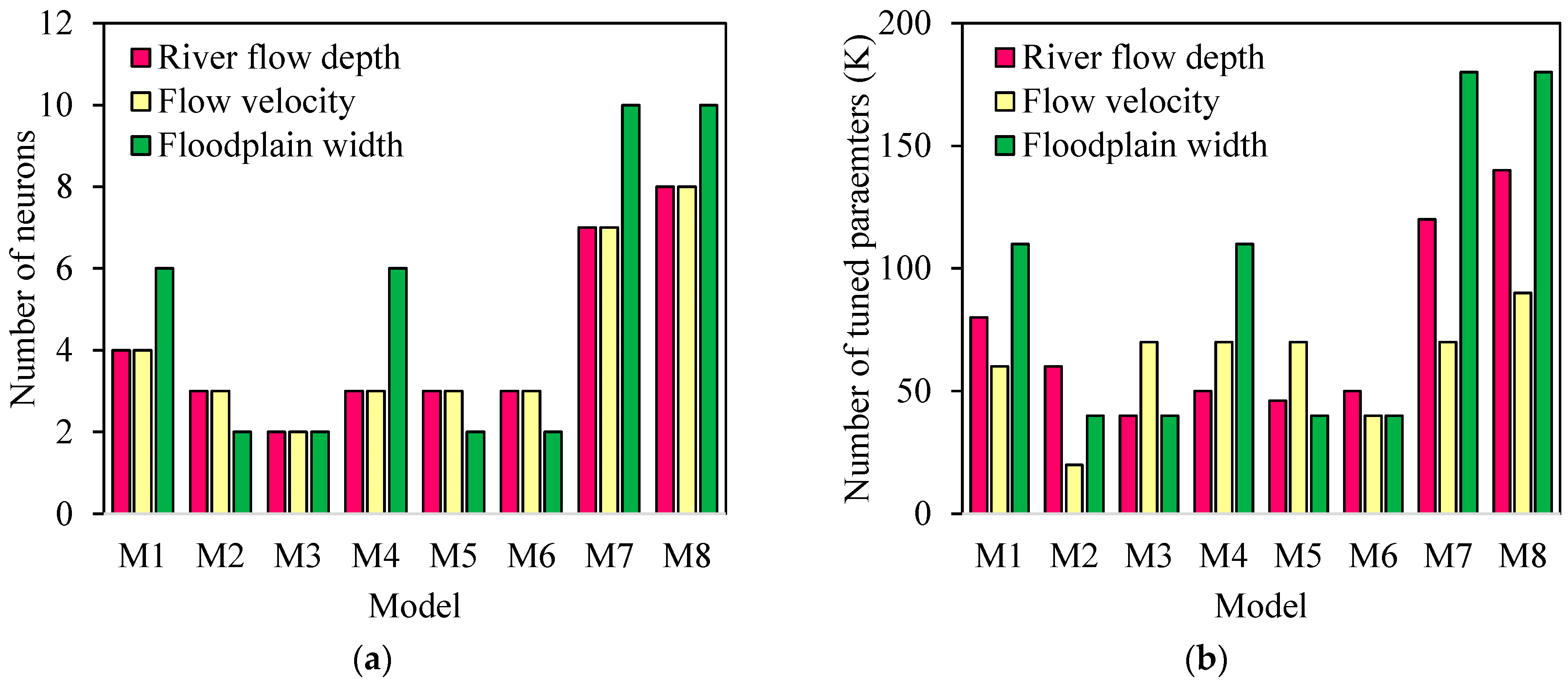
Based on the structures presented in Figure 7, it is evident that the complexity of the models varies not only in terms of the number of neurons in each layer but also in terms of the number of layers. The characteristics of these structures, including the number of neurons and the number of tuned parameters (K in Equation (14)), are provided in Figure 8. The total number of neurons for the river flow depth, flow velocity, and floodplain depth prediction models is 33, 355, and 40, respectively. Among the eight models presented using EFGMDH for predicting various variables, 50% of the models related to floodplain width exhibit the highest complexity, while the remaining two variables (river flow depth and flow velocity) have the highest complexity percentage of 25%.

Table 3. The results of the reliability analysis for the developed EFGMDH-based models at the testing stage.

Parameter	β (Equation (17))	M1	M2	M3	M4	M5	M6	M7	M8
River flow depth	1%	83.42	5.03	61.31	59.30	66.83	67.84	80.90	84.42
	2%	96.98	10.05	88.94	87.44	94.47	94.97	94.97	95.98
	5%	99.50	20.10	99.50	99.50	99.50	99.50	99.50	99.50
	10%	100	39.20	100	100	100	100	100	100
	15%	100	59.30	100	100	100	100	100	100
	20%	100	74.87	100	100	100	100	100	100
Flow velocity	1%	36.18	2.51	59.30	56.28	59.30	25.13	59.80	58.79
	2%	70.35	4.02	90.45	81.41	90.45	46.73	85.93	91.46
	5%	91.96	14.07	99.50	99.50	99.50	85.93	99.50	99.50
	10%	100	36.18	100	100	100	96.48	100	100
	15%	100	52.76	100	100	100	99.50	100	100
	20%	100	69.35	100	100	100	100	100	100
Floodplain width	1%	70.85	42.71	44.22	69.85	48.24	51.76	73.87	70.85
	2%	84.42	60.80	65.33	84.42	70.85	67.34	85.43	85.93
	5%	91.46	83.92	83.42	90.95	88.94	88.44	94.97	94.47
	10%	93.47	88.94	92.96	93.47	95.48	94.47	97.99	98.49
	15%	95.48	92.46	95.98	95.48	96.98	96.98	98.49	98.49
	20%	96.48	92.96	97.49	96.48	97.49	97.49	98.99	98.99

exhibits the results of the reliability analysis (RA) for the developed EFGMDH-based models at the testing stage. For developed models at floodplain width forecasting and at a β = 1%, M1 has an RA of 83.42%, indicating that 83.42% of the estimates for river flow depth have a relative error within 1%. The RA for M2 is 5.03%, which means only 5.03% of the estimates meet the 1% relative error threshold. The RAs for M3 to M8 are also relatively low, indicating that these models have limited accuracy at this β value. For β = 2%, the RAs for M1 and M3 to M8 have increased, showing improved accuracy. M2’s RA has increased as well, but it is still relatively low compared to the others. For β = 5%, M1 and M3 to M8 achieves an RA of 99.50%, which means they estimate the river flow depth with a relative error of 5% or less in 99.50% of cases. M2’s RA has improved but is still not as accurate as the other models. For β = 10% and above, all models (M1 to M8) reach a perfect RA of 100%, indicating that they provide estimates with a relative error within the specified Beta threshold. In conclusion, at low β values (1% and 2%), most models (except M1 and M2) struggle to meet the stringent accuracy requirements. Additionally, at higher β values (5% and above), all models successfully meet the accuracy criteria, providing reliable estimates of river flow depth.

For developed models at flow velocity forecasting and at a β = 1%, M1 has an RA of 36.18%, indicating that only 36.18% of the estimates for flow velocity meet the 1% relative error threshold. In addition, the RAs for M2, M5, and M7 are relatively low, suggesting that these models have limited accuracy at this β level. For β = 2%, the RAs for M1, M2, M5, and M7 have improved compared to the 1% β level. Moreover, M3, M4, and M8 show higher RAs at this β value. For β = 5%, M1, M2, M5, and M7 still have relatively low RAs, although there is an improvement compared to the lower Beta levels. In addition, M3, M4, and M8 maintain high RAs, with M8 achieving a perfect RA of 99.5%, indicating accurate estimates for most cases. For β = 10% and above, all models (M1 to M8) achieve perfect RAs of 100%, meaning they provide estimates with a relative error within the specified Beta threshold for all cases. In conclusion, several models struggle to meet the stringent accuracy requirements at low β values (1% and 2%). Moreover, at higher β values (5% and above), most models (except M1, M2, M5, and M7) successfully meet the accuracy criteria, providing reliable flow velocity estimates.

For developed models at floodplain width forecasting and at a β = 1%, M1 has an RA of 70.85%, indicating that 70.85% of the estimates for floodplain width meet the 1% relative error threshold. Moreover, the RAs for M2, M3, M5, and M6 are relatively high, suggesting that these models provide accurate estimates at this Beta level. For β = 2%, the RAs for M1, M2, M3, M5, and M6 have improved compared to the 1% Beta level. M4, M7, and M8 also show higher RAs at this Beta value. For β = 5%, all models (M1 to M8) achieve high RAs at this Beta level, ranging from 91.46% to 94.97%. In addition, M2, M3, M5, M6, M7, and M8 achieve a perfect RA of 94.97%, indicating accurate estimates for most cases. For β = 10% and above, all models continue to achieve high RAs, with some reaching a perfect RA of 100% at Beta values of 15% and 20%. In conclusion, at low β values (1% and 2%), some models have relatively lower RAs, while the others exhibit higher accuracy. Moreover, at higher β values (5% and above), all models (M1 to M8) successfully meet the accuracy criteria, providing reliable estimates of floodplain width.

To calculate the sensitivity of the optimal models for river flow depth, flow velocity, and floodplain width presented in Table A1, a Partial Derivative Sensitivity Analysis (PDSA) is applied [41,64]. In this approach, the partial derivative of the final model concerning each input variable is calculated to determine the sensitivity of the desired model to each input variable. This analysis helps identify how changes in each input variable affect the model’s output or predictions. The extent of the computed partial derivative correlates directly with its impact on the predicted outcome. Positive and negative values for a partial derivative indicate that adjusting the input parameter value results in either a reduction or escalation of the outcomes, respectively.

Four input variables for the river flow depth forecasting are based on the developed model: X, Y, the Manning coefficient at the left side of the cross-sectional area (n_Left), and flow discharge (Q) (Figure 9). Generally, sensitivity values demonstrate an ascending pattern as the X values increase, with the lowest sensitivity value corresponding to the initial point and the highest value linked to the farthest point. Negative sensitivity values indicate an indirect correlation between X changes and the river flow depth value. Thus, if the variable’s value is lower than the actual value, the predicted river flow depth derived from the EFGMDH-based relationship will decrease. Conversely, it will increase if the variable’s value is higher than the actual value. Based on the provided data, it seems like the sensitivity values for river flow depth are generally small (in the range of −3 × 10⁴ to 10⁻⁴). This suggests that small changes in the input variable X have a relatively minor effect on the model’s prediction for river flow depth. The sensitivity of the developed model for the river flow depth forecasting to variable Y is comparable to the sensitivities observed for variable X, with a sensitivity range between −0.0008 and 0.0004. As depicted in Figure 1, when Y = 0, it is associated with Z1, and as the Y values decrease, they correspond from Z2 to Z9. The sensitivity values for the higher Y values are negative, but the sensitivity gradually shifts towards the positive values as the Y values decrease. This implies that at higher Y values, changes in Y have an indirect relationship with river flow depth, whereas, at lower Y values, the relationship becomes more direct. Specifically, an increase in the variable Y leads to a decrease in the calculated river flow depth at the highest Y value according to the developed EFGMDH model. Conversely, as the Y values decrease, an increase in Y results in an increase in the estimated river flow depth. It is essential to note that at the lowest Y value, the sensitivity exhibits both negative and positive aspects. The sensitivity analysis of the introduced EFGMDH-based model for river flow depth reveals that it shows positive sensitivity to both the n_Left and flow discharge across all ranges of the Manning coefficient. This implies that reducing the value of either of these variables will result in a decrease in the estimated river flow depth. However, the main distinction lies in the magnitude of sensitivity between these two input variables. The sensitivity value is relatively low for flow discharge but significantly higher for the Manning coefficient. Consequently, the developed model exhibits the most heightened sensitivity to changes in the Manning coefficient compared to the other input variables.

Developed flow velocity forecasting using the EFGMDH-based technique involves five input variables: X, Y, Slope, the Manning coefficient at the middle of the cross-sectional area (n_Middle), and flow discharge (Q). A sensitivity analysis was performed on the model’s input variables, revealing that the Manning coefficient exhibited the highest absolute sensitivity compared to the other variables. In contrast, the sensitivities of the other input variables were relatively lower. Both X and Y (representing the desired zone location), as well as slope, showed mixed positive and negative sensitivities across their respective ranges. Notably, for X, the sensitivity increased in the middle zones (Z4 and Z5), where all the sensitivities were positive. Conversely, the sensitivity decreased for Y as the desired zone location moved toward the lower zones. At the last zone (Z9), the sensitivity of the model to X was utterly negative, indicating that an increase in X resulted in an enhancement in the calculated flow velocity via the developed model. The model’s sensitivity to the Manning coefficient at the middle of the cross-sectional area (n_Middle) consistently exhibits negative values across all ranges of this variable. This means that an increase in the Manning coefficient decreases the estimated flow velocity via the developed EFGMDH-based model. Furthermore, it is essential to note that as the value of the Manning coefficient increases, the sensitivity ranges of the desired variables reduce. Specifically, the maximum absolute sensitivity value decreases from 18 to 8. This indicates that higher values of the Manning coefficient led to a narrowing of the sensitivity range for the model’s output variables, implying reduced variability in the model’s predictions. The sensitivity of the model to flow discharge is the same as the n_Middle with the difference being that all sensitivity values are positive, and the changing trend of this variable has a direct relationship with the changes in flow velocity.

Developing the EFGMDH-based model for floodplain width forecasting involves five input variables: X, Y, Slope, the Manning coefficient at the left of the cross-sectional area (n_Left), and flow discharge (Q). In the beginning and end zones, the sensitivity of the model to Y is negative, while this value is positive in the middle zones. For variable X, except for Z1, the sensitivity value is positive for the initial and middle zones and Z9 as the last zone, while this value is negative for Z7 and Z8. For slope, the sensitivity in the final zone is strongly positive, so that its value is the highest compared to the sensitivity in all slope values and even the sensitivity of the model to the other parameters. In slope values less than 0.5, the sensitivity is distributed in two ways, positive and negative, so it is impossible to accurately check the model’s behavior concerning the changes in this variable in this range. For both the Manning coefficient and flow discharge, the sensitivity is distributed positively and negatively, with the difference being that the model’s sensitivity to the Manning coefficient is significantly higher than the flow discharge. For both variables, the sensitivity in the middle values is almost lower than the small and large values of these two variables. The comparison of the model’s sensitivity to all variables shows that the developed model based on EFGMDH for floodplain width forecasting has the highest sensitivity to the Manning coefficient and slope, and its value is almost negligible for the other variables.

4. Conclusions

This study has delved into the significant impact of climate change on flooding events within the Ottawa River Watershed. Notably, the occurrence of unprecedented floods, exemplified by the 2019 event surpassing a 100-year flood magnitude, underscores the urgency of developing effective strategies. Addressing this challenge necessitated the integration of advanced numerical modeling and machine learning techniques. This approach employed an expansive dataset of river flow discharge generated by implementing a sophisticated numerical model. This dataset encompasses a diverse spectrum of potential future flooding scenarios. Building upon this foundation, the Expanded Framework of Group Method of Data Handling (EFGMDH) has been devised, a novel model that provides decision-makers with actionable equations for estimating three pivotal hydrodynamic variables: river flow depth, flow velocity, and floodplain width. The primary outcomes of the present study can be summarized as follows:

➢

According to the numerical model’s results, the floodplain width has the potential to expand significantly, ranging from 131 m to 2706 m.

➢

The optimal model for river flow depth incorporates three key input variables: the location of the desired cross-section, the Manning roughness coefficient at the middle of the river section, and flow discharge. The optimal model of flow velocity includes all the variables used in the optimal model for river flow depth as well as the river slope. Similarly, the input variables influencing the floodplain width forecasting closely resemble those for river flow depth, with the sole distinction being the utilization of the Manning roughness coefficient on the left side of the channel rather than the middle.

➢

The average relative error of the optimal models is impressively low, staying below 4%. Specifically, it stands at approximately 1% for the floodplain width and river flow depth, whereas it reaches 3.3% for the flow velocity.

➢

The reliability analysis revealed that the developed model for river flow depth forecasting exhibits a remarkable forecasting ability, with a maximum relative error of 1%, 2%, and 5% observed in more than 61%, 88.94%, and 99.5% of all samples, respectively. Similarly, the developed model demonstrates a strong forecasting ability for flow velocity, achieving a maximum relative error of 1%, 2%, and 5% in 59.3%, 90.45%, and 99.5% of all samples, respectively. Regarding the floodplain width, approximately 93% of all samples are estimated with a relative error of less than 10%, while an impressive 97.5% of all samples exhibit a relative error of less than 20%.

➢

The outcomes of the sensitivity analysis indicate that the models devised for forecasting flow velocity and river flow depth are notably sensitive to the changes in the Manning coefficient. This variable substantially impacts the predictions, while the sensitivity to the other input variables is relatively insignificant. Similarly, the model formulated for floodplain width forecasting demonstrates a high sensitivity to the variations in both the Manning coefficient and river slope. In contrast, the sensitivity of this model to the other variables in the predictions is relatively minor compared to these two key factors.

While this study provides site-specific insights into the Ottawa River Watershed, its implications extend far beyond. The amalgamation of numerical modeling, machine learning, and rigorous analysis yields findings that offer valuable lessons for addressing flood dynamics in a changing climate. By emphasizing these broader lessons, it aims to contribute to the collective efforts of researchers, practitioners, and policymakers working toward more resilient and informed flood management strategies worldwide.