Article

Urban Flood Modelling under Extreme Rainfall Conditions for Building-Level Flood Exposure Analysis

by
Christos Iliadis
1,*,
Panagiota Galiatsatou
2,3,*,
Vassilis Glenis
1,
Panagiotis Prinos
2 and
Chris Kilsby
1
1
School of Engineering, Newcastle University, Newcastle Upon Tyne NE1 7RU, UK
2
Hydraulics Laboratory, School of Civil Engineering, Aristotle University of Thessaloniki (AUTh), 54124 Thessaloniki, Greece
3
Department of Geoinformatics, Surveying and Hydraulic Modelling, Executive Division of Strategic Planning and Development, EYATH S.A., 54622 Thessaloniki, Greece
*
Authors to whom correspondence should be addressed.
Hydrology 2023, 10(8), 172; https://doi.org/10.3390/hydrology10080172
Submission received: 18 June 2023 / Revised: 8 August 2023 / Accepted: 14 August 2023 / Published: 17 August 2023

Abstract

:
The expansion of urban areas and the increasing frequency and magnitude of intense rainfall events are anticipated to contribute to the widespread escalation of urban flood risk across the globe. To effectively mitigate future flood risks, it is crucial to combine a comprehensive examination of intense rainfall events in urban areas with the utilization of detailed hydrodynamic models. This study combines extreme value analysis techniques applied to rainfall data ranging from sub-hourly to daily durations with a high-resolution flood modelling analysis at the building level in the centre of Thessaloniki, Greece. A scaling procedure is employed to rainfall return levels assessed by applying the generalised extreme value (GEV) distribution to annual maximum fine-temporal-scale data, and these scaling laws are then applied to more reliable daily rainfall return levels estimated by means of the generalised Pareto distribution (GPD), in order to develop storm profiles with durations of 1 h and 2 h. The advanced flood model, CityCAT, is then used for the simulation of pluvial flooding, providing reliable assessments of building-level exposure to flooding hazards. The results of the analysis conducted provide insights into flood depths and water flowpaths in the city centre of Thessaloniki, identifying major flowpaths along certain main streets resulting in localised flooding, and identifying around 165 and 186 buildings highly exposed to inundation risk in the study area for 50-year storm events with durations of 1 h and 2 h, respectively. For the first time in this study area, a detailed analysis of extreme rainfall events is combined with a high-resolution Digital Terrain Model (DTM), used as an input into the advanced and fully featured CityCAT hydrodynamic model, to assess critical flowpaths and buildings at high flood risk. The results of this study can aid in the planning and design of resilient solutions to combat urban flash floods, as well as contribute to targeted flood damage mitigation and flood risk reduction.

1. Introduction

Urban surface water floods are amongst the most widely distributed natural hazards, endangering lives and causing damage to properties worldwide. The extent and severity of the damage is a product of both the intensity and duration of extreme rainfall events (variable in space and time), and their interaction with the complex flowpaths in a city on the ground surface and below it [1]. Impermeable surfaces in urban areas, impeding infiltration and creating overland flow which exceeds the drainage capacity of the existing infrastructure, renders cities vulnerable to flash floods. Climate change and urbanisation are expected to increase urban flood risk, contributing to different components of the flooding system. Climate change, associated with global warming and an increase in the frequency and severity of extreme weather events, is anticipated to intensify flooding hazards. Urbanisation will contribute to the increase in flooding hazards, caused by a decrease in infiltration, baseflow and lag times and an increase in runoff volumes and peak discharges [2,3], but also to the increasing impacts of urban floods (increase in potential flood damages) caused by the growth of settlements and assets in flood-prone areas followed by a rise in property value in such areas [4,5].
Nowadays, urban floods affect both developing and developed countries, with the impacts of pluvial flooding being a major problem due to frequent natural disasters in urban areas [6]. Flood damage mitigation in urban areas includes both structural and non-structural measures. Structural measures involve urban flood defences and flood control structures or designing or upgrading stormwater and drainage networks. Non-structural measures mainly focus on flood early warning systems and preventive actions [5,7]. Urban flood modelling combined with exposure assessment of the buildings and population affected represents a principal non-structural measure to effectively manage urban flooding events and their adverse effects, as well as a prerequisite for disaster prevention and mitigation.
Flood modelling is a powerful tool in understanding the hydrodynamics of historic flood events, and in some cases, the construction of accurate IDF (intensity–duration–frequency)/DDF (depth–duration–frequency) curves can be used to predict future events that will cause damage to the urban fabric [8]. There exist several studies combining flood inundation modelling with hydrological modelling and the unit hydrograph theory, mainly focusing on fluvial flooding in small or larger catchments [9,10,11,12,13,14], using DEMs (Digital Elevation Models) or DTMs (Digital Terrain Models) with a computational grid resolution ranging between 5 m and 100 m. However, it should be noted that the combination of an incorrect representation of urban features in the flood model such as buildings, bridges, infrastructure, etc., and the resampling of the DEM/DTM multiple times might cause large inconsistencies [1,15,16] and overestimation of the flooding hazard in areas with minor inundation issues and vice versa. Unlike studies modelling fluvial flood inundation in urban areas, studies focusing on the exposure assessment of urban areas to pluvial floods are rather limited, and started receiving significant interest quite recently. Zhu et al. [17] used the LISFLOOD-FP hydrodynamic model to simulate flooding in Lishui City, China, and employed the building-scale population distribution map to assess the population affected. Park et al. [5] evaluated flood risk for different building types, conducting vulnerability and exposure analysis in five regions of Ulsan City, South Korea. Their analysis resulted in a classification of each building type into five risk-related classes. Stefanidis et al. [18] presented a coupling of hydrological and hydraulic modelling on a national scale to produce flood hazard maps regarding flooding exposure in residential areas and infrastructure in Greece. Bertsch et al. [19] presented a sensitivity analysis and validation of a generic flood exposure analysis following a large storm event in Newcastle upon Tyne, UK, where more than 70% of the inundated buildings in the area were correctly identified during the storm event.
Pluvial flood risk assessment in urban areas, associated with estimating the hazard, exposure, and vulnerability components for the affected system, is therefore a major challenge for future societies. Τhere is a great need to combine hydrological and hydrodynamic modelling to understand the impacts of urban floods, the water flowpaths in a city, and the urban features exposed to high flood risk. This study combines a detailed analysis and modelling of extreme rainfall events in the centre of Thessaloniki, Greece, with an advanced hydrodynamic model, CityCAT, to simulate pluvial flooding, significantly assisting a reliable assessment of exposure to flooding. The results of this study can aid in the planning and design of resilient solutions against urban flash floods, as well as contributing to targeted flood damage mitigation and flood risk reduction.
CityCAT has previously been applied in studies in the UK [1,19,20,21,22] and the USA [23] (Environmental Justice of Urban Flood Risk and Green Infrastructure Solutions-Urban Systems Lab, Urban Flooding, Equity, and Green Infrastructure (arcgis.com, accessed on 10 July 2023)), where detailed and reliable spatial datasets were available, such as DTMs, building footprints, green spaces, and roads. This study also aims to demonstrate and assess the universal applicability of CityCAT, even in regions where comparable datasets may not be readily available, emphasising the value of integrating the model with extreme rainfall data to enhance flood resilience in urban areas. The practical implementation of the model in this study will assist local authorities and engineers in improving their future flood adaptation strategies. This study also marks the first published implementation of a flood exposure analysis calculator at the building level in a large Greek city, as opposed to conventional assessments limited to flood zoning.

2. Materials and Methods

2.1. Study Area and Available Datasets

The historic centre of Thessaloniki city in Greece was the study area of the present work, located in the northern part of Greece. Thessaloniki is part of the municipality of Central Macedonia, and it is the second largest city in Greece with a population of around 814,000 (Thessaloniki Population 2023: worldpopulationreview.com, accessed on 5 June 2023). The dense city centre facing the coastal front is characterised by historic buildings, residential properties, marketplaces, and a few green open spaces (see Figure 1). This part of Thessaloniki has suffered from severe storms and flash floods in the last decade, causing significant damage to roads, basements, local stores, etc. It should be noted that, during storm events, the roads are seen to become the main flowpaths for floodwater.
Two different datasets are available in the study area for the analysis of extreme rainfall events. The first dataset consists of daily rainfall data at AUTh (Aristotle University of Thessaloniki) station located in the centre of the city and covering 64 years (1958–2021) of measurements (no missing data are present), obtained from the database of the School of Geology, AUTh. The second dataset includes monthly maximum rainfall depths for rainfall durations of 5 min, 10 min, 15 min, 30 min, 1 h, 2 h, 6 h, 12 h and 24 h at Mikra station, located in the eastern part of the city. This dataset was made available by the Hellenic National Meteorological Service (HNMS) and covers a period of 25 years (1963–1987). It is therefore evident that the second dataset includes rainfall measurements of finer temporal scales than the first one, but it contains only monthly maximum values, and its length is significantly shorter than that of the daily rainfall series available at AUTh. It should also be noted that the second dataset contains missing values. To proceed with the extreme value analysis of all available datasets, annual maxima were first extracted for both the daily and the sub-daily series, and each dataset was tested for stationarity and trends [24]. The datasets examined satisfy the hypothesis of stationarity, while no statistically significant trends were detected.

2.2. Extreme Rainfall Assessment

Extreme value theory includes two main approaches for identifying and modelling the extreme values of a random process, namely the block-maxima approach where the extremes follow a generalised extreme value (GEV) distribution, and the peaks-over-threshold (POT) approach that fits the extremes using a generalized Pareto distribution (GPD). In the former approach, the observation period is divided into nonoverlapping equal intervals (of length usually equal to one year) and block maxima are selected to be fitted according to a GEV distribution [24]:
G x ; μ , σ , ξ = exp 1 + ξ x μ σ 1 ξ ,   ξ 0 exp exp x μ σ ,   ξ = 0  
where μ, σ and ξ are the location, scale and shape parameters of the distribution, respectively. The POT approach employs two probability distribution functions: one for the intensity of exceedances over an appropriately defined threshold, typically a GPD, and another for the number of events per year (typically a Poisson distribution, or alternatively a constant number is used). The cumulative distribution function of the GPD is given by [24]:
G x ; σ , ξ , u = 1 1 + ξ x u σ 1 ξ ,   ξ 0 1 exp x u σ ,   ξ = 0  
where σ and ξ are the scale and shape parameters of the GPD, respectively, while u is the defined threshold value. The scale parameter of the GPD, sometimes referred to as the modified scale parameter, is expressed as a function of the respective GEV scale parameter as:
σ G P D = σ G E V + ξ u μ
considering that the shape parameter, ξ, of the GPD is equal to that of the corresponding GEV. The GPD-Poisson, which employs the Poisson distribution to model the number of exceedances over the threshold value per year, is characterized by three parameters, the exceedance rate, λ, the scale, σ, and the shape, ξ, parameters.
Considering the threshold of the POT approach, a high value improves the validity of the asymptotic approximation of the GPD, but at the same time increases the variance of parameter estimates because of the reducing dimensions of the excess sample. In contrast, a very low threshold may increase bias from model misspecification [25,26]. Finding a trade-off between these two issues is critical in fitting an extreme value distribution and producing reliable estimates of extremes. The parameters of the extreme value distributions were assessed using both maximum likelihood estimation (MLE) and the L-moments [27] approach.

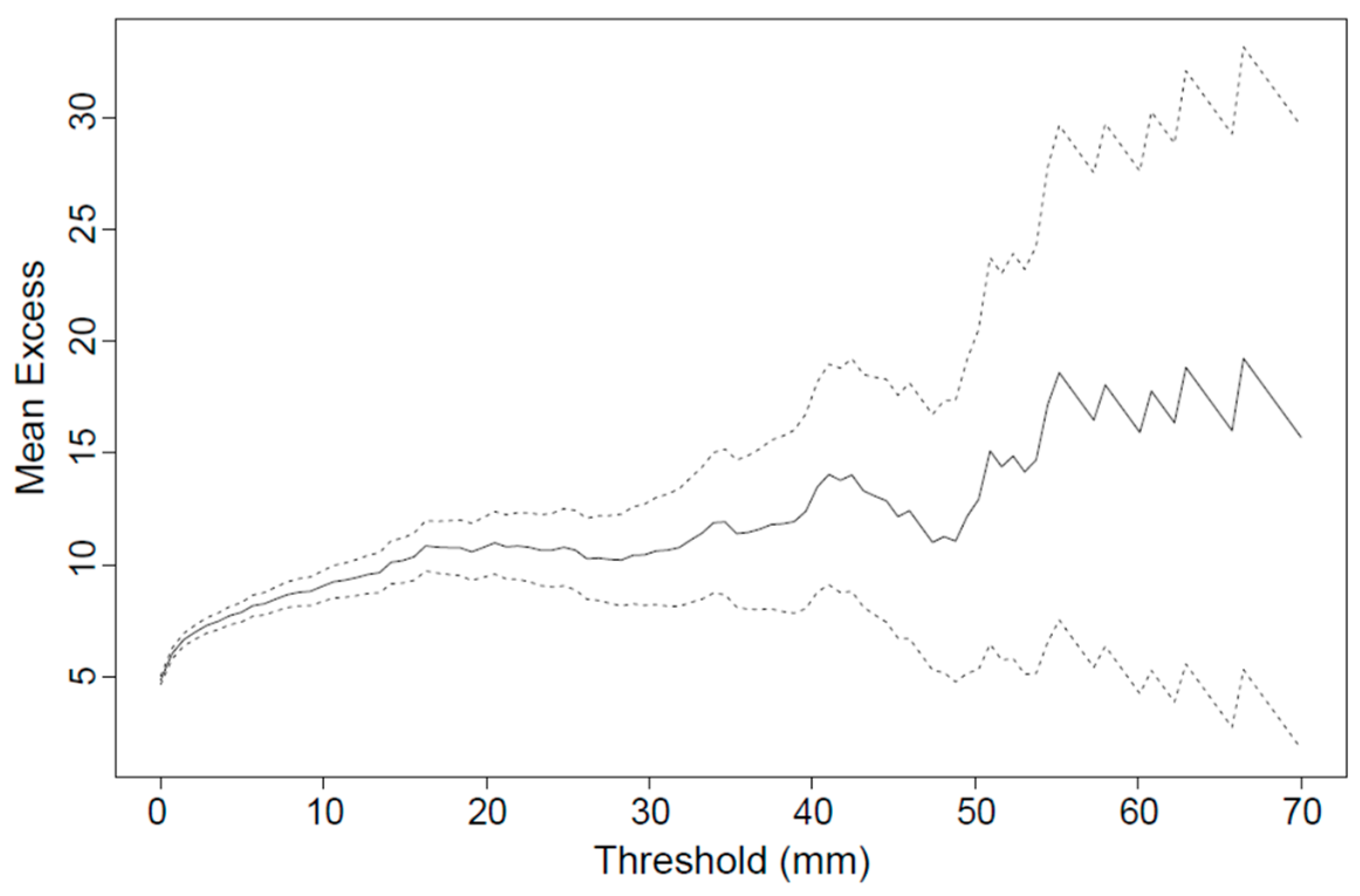
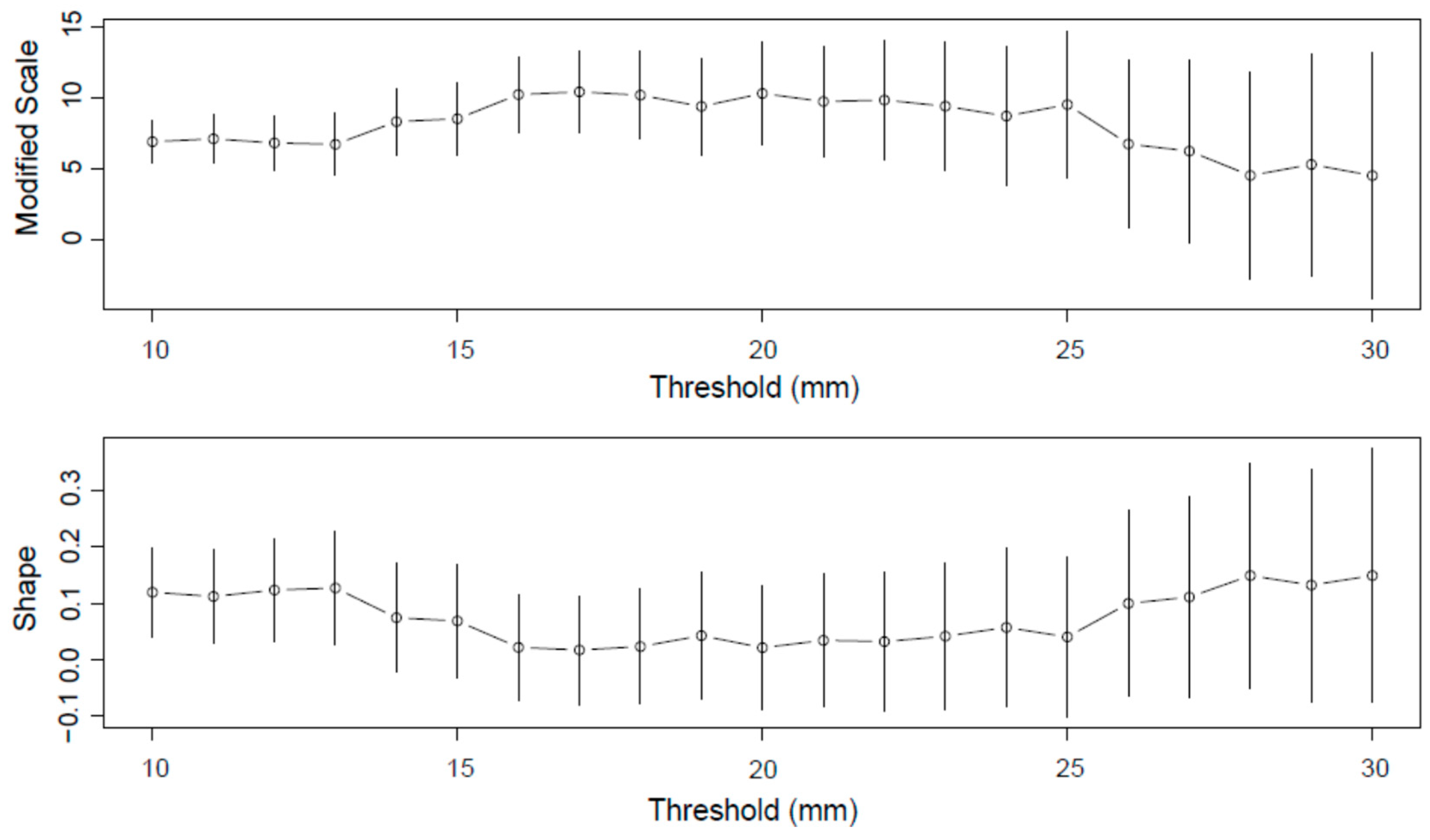
2.2.1. POT Threshold Selection

When the POT approach is used to model rainfall extremes, an appropriate threshold should be selected to detect exceedances and define the extreme sample. Various threshold selection methods have been proposed in the literature, such as empirical methods, distance measure approaches, or diagnostic plots such as the mean residual life plot and GPD parameter estimate stability plots [28]. However, these approaches have a significant level of subjectivity in the threshold selection process. This work used two methodologies, aiding in creating a more automatic threshold selection process [29]. These threshold selection methods were proposed by Bader et al. [30] (henceforward referred to as threshold selection method (a)) and Silva Lomba and Fraga Alves [31] (henceforward referred to as threshold selection method (b)) facilitating a less ambiguous and more objective selection of daily extreme rainfall events.
Threshold selection method (a) [30] considers a set of candidate thresholds u1 < … < ul, each having ni exceedances, i = 1, …, l. Let H0(i) denote the null hypothesis that the distribution of ni exceedances above the threshold ui follows the GPD. Following the forward stop rule of G’Sell et al. [32], a rejection rule was constructed by returning a cutoff level k ^ , such that H1 to H k ^ are rejected:
k ^ = m a x k 1 , , l : 1 k i = 1 k l o g 1 p i a
where a is a prespecified significance level and pi I = 1, …, l are the corresponding p-values of the l hypotheses. If there is no k ^   [1, …, l], there is no rejection of the null hypothesis.
The p-values in Equation (4) are assessed using the Anderson–Darling (AD) test for each candidate threshold, with the respective statistic assessed as:
A n 2 = n 1 n i = 1 n 2 i 1 l o g z i + l o g 1 z n + 1 i
where z i = F y i θ ^ n is the probability integral transformation of the order statistics of the exceedances y(1) ≤ … ≤ y(n), based on the maximum likelihood estimator of θ, θ ^ n , under the null hypothesis H0. F denotes the cumulative distribution function of the GPD for each candidate threshold.
Threshold selection method (b) [31] is based on L-moments. For the random variable X with distribution function F, the theoretical L-moments λr+1 with r = 0, 1, … are expressed as linear functions of the specific probability weighted moments (PWM):
a r = M 1,0 , r = E X 1 F X r
with the dimensionless L-moment ratios L-skewness, τ3 = λ32, and L-kurtosis, τ4 = λ4/λ2, calculated as functions of the L-scale, λ2, and the third, λ3, and fourth, λ4, L-moments, respectively. Let ar be the unbiased estimator of ar for an ordered sample x1:n ≤ … ≤ xn:n:
a r = 1 n   i = 1 n n i r x i : n n 1 r 1 ,   r = 0 ,   1 , ,   n 1
with the unbiased sample L-skewness, t3 = l3/l2, and L-kurtosis, t4 = l4/l2, calculated as functions of the sample L-scale, l2, and the third, l3, and fourth, l4, sample L-moments, respectively.
A set of candidate thresholds u i i = 1 I are first defined with I = 10 or 20 sample quantiles. The minimum Euclidean distance is then defined between the sample L-skewness, τ 3 , u i , and L-kurtosis, τ 4 , u i , for each threshold value and the respective quantities of the theoretical GPD curve:
d u i = min τ 3 t 3 , u i τ 3 2 + t 4 , u i g τ 3 2 ,   for   i = 1 , ,   I ,   with   g τ 3 = τ 3 1 + 5 τ 3 5 + τ 3
The best candidate threshold is then defined as:
u * = argmin u i , 1 i I d u i
characterized by L-moment statistics that fall closer to the respective values of the theoretical L-moment ratio curve.

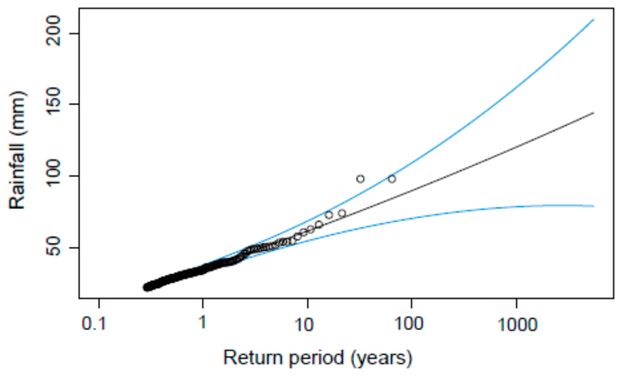
2.2.2. Scaling Rainfall Extremes
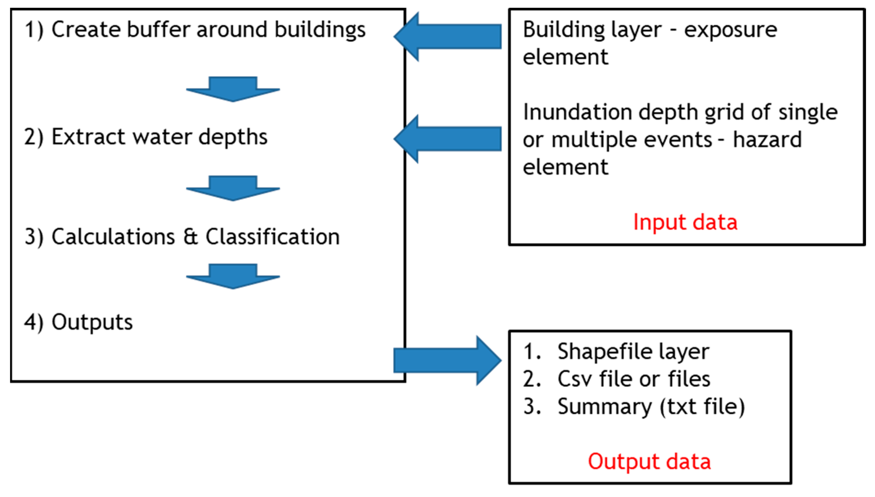
Rainfall features of different temporal scales can be linked using scaling models, mainly based on the multifractal behaviour of rainfall. Temporal downscaling and temporal disaggregation methods are used to produce finer-temporal-scale rainfall data from coarser resolution observations. Temporal downscaling usually refers to the generation of data of a high temporal resolution by means of statistical techniques, most commonly stochastic models, calibrated using information on the statistics of data from lower resolution temporal scales. Temporal disaggregation indicates the generation of high-resolution temporal data based on coarser time scales, so that the former add up to the totals of the second scale. This can be performed by means of a temporal partitioning of low-temporal-resolution amounts using a recursive rule or by repeatedly adjusting stochastic models to the generated high-resolution data. Within the general framework of temporal disaggregation, different methodologies have been developed in the literature. Some quite simple techniques, based on assumptions regarding the association of specific characteristics of the probability distribution functions of rainfall amounts at different time scales, have been developed by Liu and Wang [33] and Chen et al. [34,35], among others. However, these techniques do not represent the basic statistics of the fine temporal scales of precipitation in a satisfactory way, nor the intermittency of precipitation events. Precipitation stochastic generators are also utilized for temporal disaggregation purposes of rainfall amounts. Methods based on point-process models for the temporal disaggregation of hydro-meteorological data are quite widespread, producing satisfactory results [36,37,38,39,40]. Lee et al. [41], Salas and Lee [42] and Lee and Jeong [43] introduced a nonparametric model for the temporal disaggregation of hydro-meteorological variables, which incorporates k-nearest-neighbour resampling and a genetic algorithm. Temporal disaggregation of hydro-meteorological data is also performed by means of machine learning techniques (i.e., Kumara et al. [44]).
The hypothesis of scale invariance [45] is usually applied to link rainfall intensities of different temporal scales. More specifically, the hypothesis of scale invariance states that annual maximum rainfall intensities, Id and Iλd, corresponding to durations d and λd, respectively, can be related by the following equation [46,47,48]:
I λ d = λ β I d
where equality corresponds to the similarity of probability distributions. The coefficient λ is the ratio of scale invariance between the known duration D and the duration to be assessed, d, and β is the self-similarity index of the studied rainfall process. The qth moments of rainfall intensity are obtained from Equation (10) as follows [46]:
E I λ d q = λ β ( q ) E I d q
where β(q) is the scale exponent of order q, estimated by log-transforming Equation (11):
l o g E I λ d q = β q l o g λ + l o g E I d q
Therefore, the exponent β can be assessed as the slope of the linear relationship described by Equation (12). The abovementioned scaling behaviour can also be detected in quantiles of rainfall intensities corresponding to durations d and λd, considering that their cumulative distribution function (CDF) has a standardized form independent of the rainfall duration [48]. In this work, a scaling procedure is applied to rainfall intensity quantiles corresponding to different durations, considering that their CDF has a standardized form independent of the rainfall duration. The scaling laws are assessed for all return periods for rainfall durations from 5 min to 30 min and from 30 min to 24 h, considering that rainfall dynamics change quite significantly in convective events.
Intensity–duration–frequency (IDF) and depth–duration–frequency (DDF) curves based on local precipitation measurements summarise the relationships between rainfall dynamics, namely rainfall intensity or depth, duration and frequency (return period), and are currently utilized for engineering design and management applications, such as flood risk protection structures and infrastructure or flood-mitigation projects. The IDF (DDF) curves are constructed for different return periods, representing the variation of rainfall intensity (depth) with duration. In this work, IDF and DDF curves were created following the methodology described in Galiatsatou and Iliadis [48]. Theoretical probability distribution functions were fitted to annual maximum or POT rainfall intensities of particular durations ranging from shorter periods, e.g., 5 min, to daily events. When annual maximum rainfall intensities (or depths) were available, the GEV distribution (Equation (2)) was fitted to the samples of different durations, and rainfall return levels were assessed as:
X T = μ σ ξ 1 l n 1 1 T ξ ,   ξ 0 μ σ ln l n 1 1 T ,   ξ = 0  
for a defined return period, T. When the GPD (Equation (2)) is fitted to rainfall POTs, the return levels are given by [24]:
X T = u + σ ξ Τ n y ζ u ξ 1 ,   ξ 0 u + σ l n Τ n y ζ u ,   ξ = 0  
where ny is the number of observations per year and ζu is the total exceedance rate of the threshold u. Confidence intervals for return levels estimated using both the GEV and GPD are assessed using the delta method [49].

2.3. Flood Exposure

An efficient flood exposure tool, developed by Bertsch et al. [19], was used to calculate the flood exposure likelihood for buildings. Figure 2 presents the schematic workflow of the flood exposure analysis tool. Each building was assessed for flood risk using simulated flood depths in a 3 m buffer zone around its perimeter, where the mean and the 90th percentile values were calculated, with the proposed value for the buffer zone (see Figure 3) depending on the resolution of the computational grid (2 m in this study). A simple classification scheme shown in Table 1 was used to categorise buildings at low, medium and high flood risk.

2.4. Modelling System and Model Set Up

Over the last decade, many studies have reviewed hydraulic and hydrodynamic models which have been developed to simulate surface flows [6,51,52,53], and one of the most advanced and fully featured is the City Catchment Analysis Tool—CityCAT (for a full description, see Glenis et al. [20]) developed at Newcastle University. CityCAT is a unique hydrodynamic model able to simulate fully coupled surface and pipe network flows, and it can represent natural drainage systems and built-up areas, with the explicit representation of buildings, where the buildings’ footprint is excluded from the computational grid, and different types of blue-green infrastructure (BGI) [20,21,22,54] (such as blue/green roofs, water butts, swales, etc.), thus enabling the assessment of different alleviation measures. The model outputs include maps and time series of water depth, flow velocity, and the volume in and out of manholes, gully drains, buildings, etc. The required inputs are: (a) a high-resolution Digital Terrain Model (DTM) to unlock the full potential of the model, although depending on urban layouts, a lower resolution model may still be very functional; (b) the buildings’ footprint; (c) green spaces to calculate the infiltration with the Green–Ampt method [55]; and (d) the IDF and DDF curves to generate storm profiles with the rainfall–runoff method [56], to be applied over the whole domain with a uniform assumption.
The flood domain studied here was modelled using CityCAT for two different design storm events, with a magnitude of 1 in 50 years and a duration of 1 h and 2 h. The buildings’ footprint was extracted from the ONEGEO data (https://onegeo.co/data, accessed on 10 May 2023) and the permeable areas from OpenStreetMap (https://www.openstreetmap.org, accessed on 10 May 2023). The computational grid was constructed using the DTM provided by the Hellenic Cadastre (http://www.ktimatologio.gr/en, accessed on 10 May 2023) at a resolution of 2 m (each cell with an area of 4 m2), so the total number of computational cells in the flow domain was 125,192, covering an area of 0.78 km2. The representation of the buildings in the model was performed following the ‘Building Hole’ approach where a non-flow boundary is generated around buildings to redistribute the rainfall to the nearest grid square (for a full description and performance relative to other methods, see Iliadis et al. [1]). Following the previously described approach, this study explored the likelihood of flood exposure for 1165 buildings. The roughness coefficient (Manning’s n) was defined as 0.02 for impermeable areas and 0.035 for permeable areas. Due to the limitations in the Hellenic National regulations in urban flood modelling, and the intended design of the combined sewer system for storms with a return period of 10 years in the city centre of Thessaloniki (based on design cross-sections of existing combined sewers), a simple assumption was made in this work, that 20% of the rainfall enters the drainage system. In other countries, i.e., the UK, there is an instruction to flood modellers, when they do not combine the drainage system with the surface, to exclude specific rainfall from the model (e.g., 6 mm–15 mm).

3. Results

3.1. Extreme Rainfall Assessment

Threshold selection for the daily rainfall data was performed using both well-known threshold selection techniques, such as the mean residual life plot (MRL) and parameter stability plots, while also accounting for site-specific characteristics of extreme rainfall, together with the two new threshold selection techniques presented in Section 2.2.1. The MRL plot of the daily rainfall sample at AUTh station is presented in Figure 4.
The MRL plot identifies a range of possible threshold values in the interval 10 mm ≤ u ≤ 30 mm. Figure 5 presents the GPD parameter stability plots for the modified scale (scale parameter of the GPD), and shape parameter, ξ, for thresholds in [10,30] mm. Based on stability characteristics of the GPD stability plots, while also considering the uncertainty of the parameters represented using 95% confidence intervals shown as vertical lines for each threshold, a threshold between 14 mm ≤ u ≤ 27 mm is considered to be a good candidate.
The threshold selection method (a) was applied for threshold values in the entire range, 10 mm ≤ u ≤ 30 mm. The significance level selected was set at 5%. The forward stop rule applied did not explicitly identify a cutoff level. However, it has been observed that the threshold u = 22 mm was the only one giving a p-value of the AD statistic lower than 5%. The threshold selection method (b) provided clearer results, indicating u = 22 mm as the threshold providing a local minimum to the Euclidean distance criterion. The threshold u = 28 mm provided the global minimum of the distance d u i in the studied interval. However, this threshold level ended up with only 134 POT samples, corresponding to just λ = 2.09 exceedances per year. Therefore, the threshold u = 22 mm was selected to perform the extreme value analysis of the daily rainfall data, corresponding to 221 POT samples, with around λ = 3.45 exceedances per year.
Using a threshold u = 22 mm, the GPD was fitted to daily rainfall maxima (Equation (2)) using both MLE and the L-moments approach, with both approaches providing consistent results, with higher return level estimates assessed using MLE. Figure 6 presents rainfall return level estimates assessed using Equation (14), with the parameters of the GPD calculated using the MLE approach. The black line represents maximum likelihood rainfall return level estimates, while the blue lines represent the upper 97.5% and the lower 2.5% confidence limits (95% confidence interval). Round marks in the return level plot correspond to measured data from the available extreme rainfall sample. It should be noted that the most extreme 24-hourly rainfall measurement was 98 mm, and was observed in 1985 and 2014. The maximum likelihood return level estimate significantly underestimates this value, while the upper 97.5% confidence limit seems to better fit the most extreme part of the observed sample. More specifically, for a return period of 64 years, equal to the daily rainfall sample length, the maximum likelihood estimate of the rainfall return level is about 84 mm, and the respective 97.5% upper confidence limit is 100.5 mm. Based on this finding, the upper 97.5% confidence limit for daily rainfall return levels was used in the scaling methodology presented in Section 2.2.2 to extract rainfall return levels corresponding to finer temporal scales.
The GEV distribution (Equation (1)) is then fitted to annual maximum rainfall intensities for time periods of 5 min, 10 min, 15 min, 30 min, 1 h, 2 h, 6 h, 12 h and 24 h, available at Mikra station for the period 1963–1987 using L-moments (due to the small sample size of this dataset). Rainfall return levels for the different durations are assessed for return periods of 2, 5, 10, 20, 50, 100, 200 and 500 years using Equation (13). For each return period, plots of Log(i) and Log(λ) are created, and linear functions are then fitted, dividing the plots into two parts, the first one corresponding to rainfall durations from 5 min to 30 min, and the second one from 30 min to 24 h. To end up with two different rainfall duration groups, a number of trials were performed considering different duration groups, and finally we selected those providing the highest coefficients of determination, R2, for all return periods. Figure 7 presents the linear relationships between the log-transformed quantiles (log-transformed return levels) of rainfall intensity and log-transformed scale factors of different durations, for return periods of 5 years (left panel) and 50 years (right panel). The plots include the linear function equations for rainfall durations in the intervals of 5 min to 30 min and 30 min to 24 h, and the respective coefficients of determination. Table 2 presents estimates of the self-similarity index (estimates of −β) assessed for all return periods and for the two groups of rainfall duration.
The self-similarity indices presented in Table 2 are then used in Equation (12) to temporally downscale daily rainfall return levels assessed from fitting the GPD to data from AUTh station (1958–2021). More specifically, daily rainfall return level estimates corresponding to the 97.5% upper confidence limit (see Figure 6) are used in the scaling process. Rainfall return level estimates extracted for durations of 5 min, 10 min, 15 min, 30 min, 1 h, 2 h, 6 h, and 12 h are used to construct IDF and DDF curves for the study site. The formulas extracted to describe the IDF and DDF curves are given below:
i m m h = 16.63 T 0.2152 t 0.7116   and   p m m = 16.63 T 0.2152 t 0.2884
where T is the return period (years) and t is the rainfall duration (h). Figure 8 presents IDF and DDF curves for Thessaloniki based on Equation (15) for return periods of 2, 5, 10, 20, 50, 100, 200, and 500 years.

3.2. Modelled Flow Depth

A detailed analysis of the areas where maximum water depths are highlighted and analysis identifying the critical roads during heavy rains will be presented in this section. The rainfall depth for 50-year events, specifically for durations of 1 h and 2 h, is evaluated. The findings indicate that the assessed rainfall depth is approximately 70% higher than the quantiles derived from the DDF curves extracted from the shorter-duration dataset spanning 25 years (1963–1987). This high difference is attributed to: (i) using the upper 97.5% confidence limit to assess daily rainfall return levels of the longer time series (1958–2021), (ii) fitting a POT model to the 64-year daily series to assess extreme quantiles, and (iii) missing observations in the shorter series perhaps leading to an underestimation of the extreme sample. To simulate these two storm events, the CityCAT model is employed. It should be noted that when selecting the duration for modelling purposes, it is essential to consider the critical duration that triggers the most significant flood response, taking into account factors such as time-to-peak and other relevant characteristics. In the case of a catchment area spanning only a few square kilometres, a duration of 1 or 2 h is often sufficient to adequately represent the hydrological processes and capture the flood dynamics effectively. These durations are typically suitable for encompassing the key rainfall patterns and associated runoff generation within the catchment, enabling accurate flood modelling and analysis. The application of the CityCAT model in simulating the two storm events (50-year events with durations of 1 h and 2 h, see Figure 9) provides valuable insights into flood depths and water flowpaths within the study area. Note that the simulated storm events here exhibit similarities to previously observed storms as reported by the Hellenic National Meteorological Service (HNMS).
The flood maps produced by the model outputs, depicted in Figure 10 (maximum flood depths), clearly identify a major water flowpath along Agias Sofias street (see Figure 1 to locate the street), where the darker blue illustrates water depths exceeding 30 cm. This indicates that the street is highly susceptible to flooding during intense rainfall events. Furthermore, the presence of small ponds in various parts of the catchment, attributed to the complex and dense topography of the area, highlights the potential for localised flooding. Identifying these ponding areas is crucial for understanding flood risk and implementing measures to minimise the impacts, such as sacrificial zones, the creation of retention ponds, the improvement of surface drainage in specific locations, or converting the impermeable pavements to permeable pavements.
The study area’s locations and roads, discussed below, have experienced substantial water buildup during intense rainfall events in the past, as reported by local authorities and residents. However, additional efforts are required to compare and confirm these observed occurrences with the results obtained through modelling. The modelled water depths of this work were calculated to estimate the maximum levels on the following roads (see Figure 1 to locate the streets): (a) Palaion Patron Germanou and Pavlou Mela. This particular area demonstrates a significant propensity for water pooling, with estimated water depths exceeding 30 cm. (b) Notably, Proxenou Koromila experiences frequent ponding, with estimated flood depths ranging from 25 cm to 41 cm. This road is particularly susceptible to water accumulation during storm events, which can lead to hazardous conditions. (c) In certain parts of Mitropoleos street, water depths exceeding 25 cm have been estimated. This poses a risk of localised flooding which would result in traffic disruption.
The estimated water depth and the flow direction for the two storms with 1 h and 2 h durations can be seen in Figure 11, Figure 12 and Figure 13, where we zoom in on these areas. Overall, the contribution of a detailed flood model, such as CityCAT, is crucial to developing a better understanding of the flood dynamics, quantifying water depths with high accuracy, and locating areas at high flood risk to improve inundation resilience in dense cities.

3.3. Exposure Likelihood to Buildings

In order to identify the urban features exposed to flood risk, an innovative tool was used, as described in Section 2.3. The analysis of flood exposure to buildings in the study area provides valuable insights into the vulnerability of urban features to flood risk. Note that this area has faced inundation issues from extreme events in the past, for which no formal reports exist, but are well known by local people.
Table 3 provides the total number of inundated buildings per scenario in the study area. The number of buildings classified as being at high risk for the first storm event (1 h duration) is 165, and that for the second storm event (2 h duration) is 186. These values are nearly twice as high as for the buildings with medium flood exposure. Most of the high-risk buildings are located on the streets mentioned in Section 3.2, where the flood depth is more than 30 cm. Furthermore, in the studied area of the city centre, many buildings house businesses, particularly on their ground floor, often containing vulnerable assets, while there also exist numerous buildings of historical value.
Figure 14 illustrates the flood depths and the resulting flood exposure of buildings during the two generated storm events (50-year storm events with durations of 1 h and 2 h). The use of colour-coded zones helps to categorize buildings based on the flood depths in the buffer zone. The red-coloured buildings indicate high-risk, where the flood depth exceeds the 30 cm threshold. These buildings are estimated to be more vulnerable to damage from flooding, and it is crucial to prioritize them for adaptation measures and enhance their resilience to future flooding. Buildings depicted in orange indicate a medium risk of flooding, where damage from flooding is still significant. Lastly, a grey colour highlights the buildings at low risk, with minimal flood depths and lower vulnerability to flooding.
It should be noted that further investigation is needed into the 30 cm threshold to categorise buildings according to their flood risk, in order to provide more accurate estimations to understand the risk and the vulnerability profile of the city’s buildings.

4. Conclusions

This study combines a detailed contemporary analysis of extreme rainfall events in Thessaloniki, Greece, with an advanced hydrodynamic model to simulate pluvial flooding, assisting in the reliable assessment of building exposure to flooding risks. A dual scheme is employed to assess extreme rainfall: (i) extreme daily rainfall, resulting from a long daily series, is analysed using a GPD. Two threshold detection methods are applied, to assist a less ambiguous selection of daily extreme rainfall events. (ii) Extreme rainfall of shorter annual maximum series ranging from sub-hourly to sub-daily durations is analysed using the GEV distribution. A scaling procedure is applied to rainfall return level estimates assessed from (ii), and the resulting scaling laws are applied to the more reliable daily rainfall return levels of (i), in order to finally derive storm profiles with durations of 1 h and 2 h. The resulting storm profiles are used to drive the hydrodynamic model CityCAT to simulate flooding, estimate the water depths, identify the critical water flowpaths and finally assess the total number of inundated buildings through a novel exposure analysis calculator per extreme rainfall scenario in the historic centre of Thessaloniki. Furthermore:
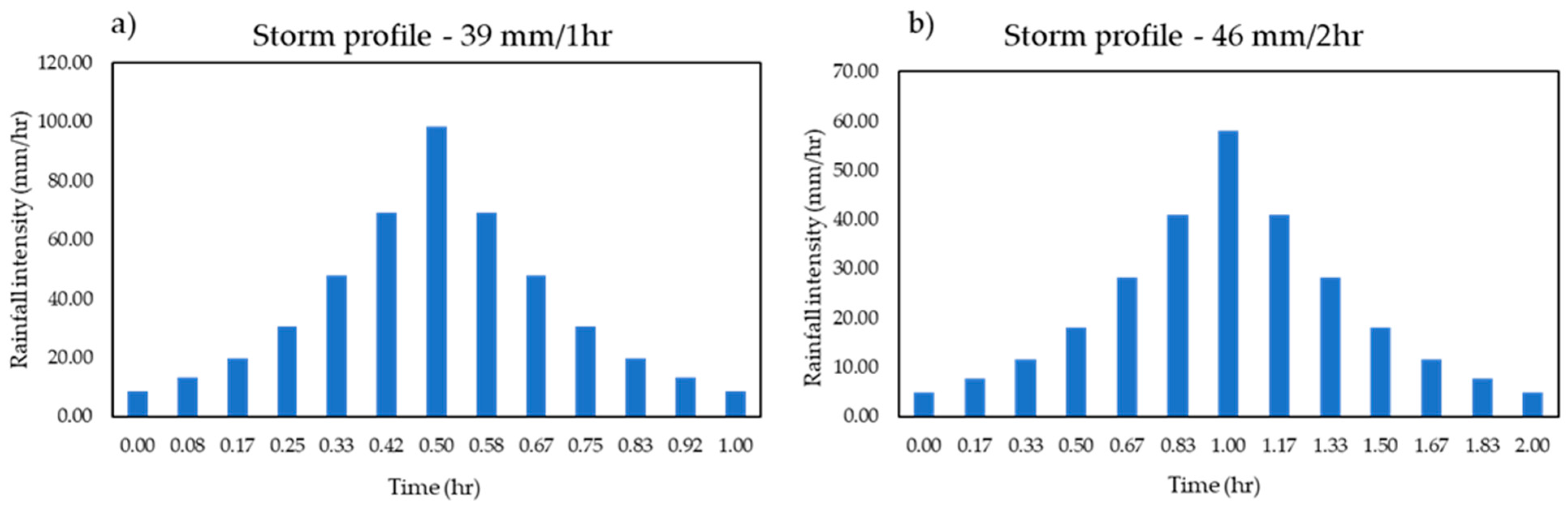
  • Typical storm events have durations spanning 1 h to 2 h, so both durations have been used here to see how sensitive the damages are to storm duration. For storms of the same return period, a modest increase is found for the 2 h storm relative to the 1 h storm.
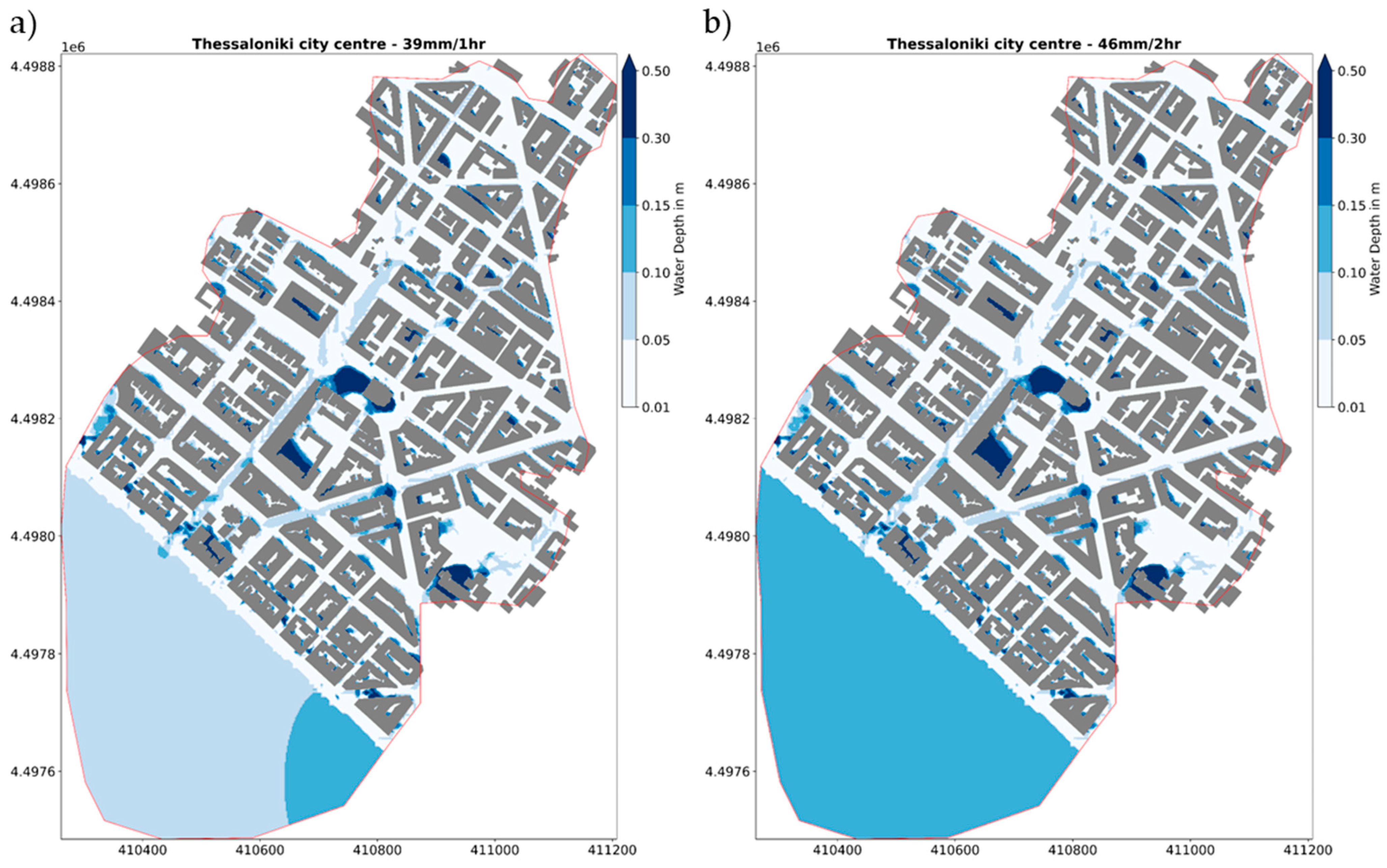
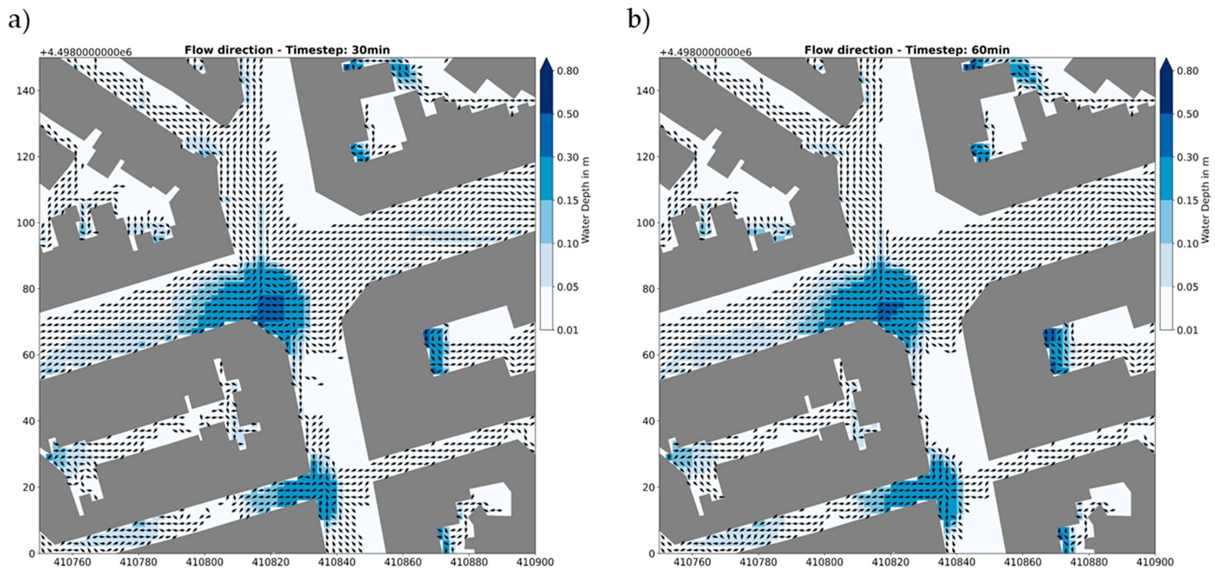
  • The CityCAT model provides valuable insights into flood depths and water flowpaths, identifying a major water flowpath along Agias Sofias street, which is highly susceptible to flooding during intense rainfall events. The presence of small ponds in various parts of the studied catchment further highlights the potential for localised flooding.
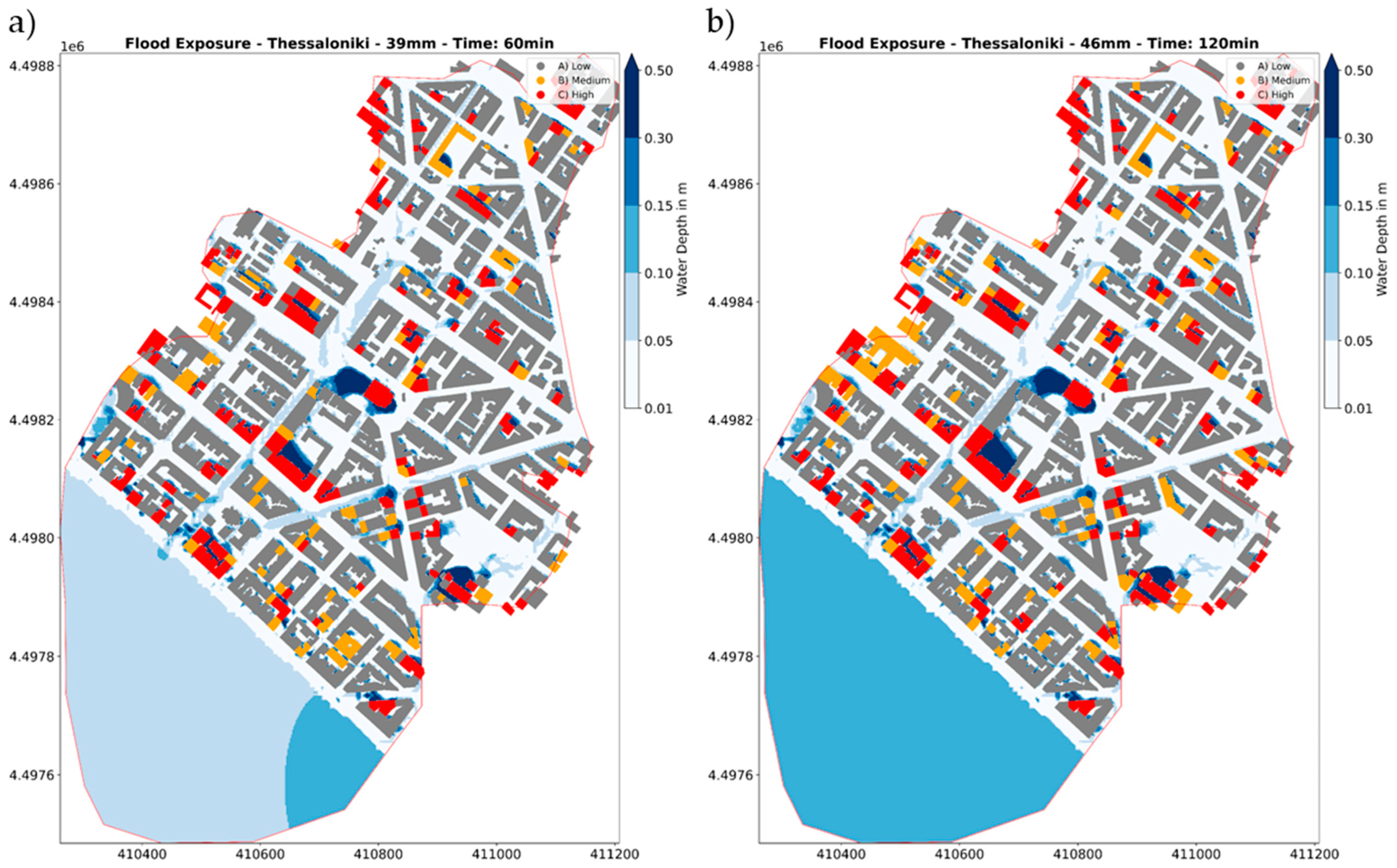
  • The estimated likelihood of flood exposure to buildings reveals the vulnerability of urban features to flood risk. Due to the previous flood events in the area, the number of buildings at high risk for both storm events underscores the importance of addressing flood impacts on the built environment.
  • The modelling system is suitable for assessing the performance of flood-resilience strategies such as retention ponds, surface drainage improvements, and permeable pavements.
This study showcases the unique capabilities of CityCAT in its application to a country like Greece, which faces challenges of limited data availability. By leveraging globally accessible datasets, a high-resolution Digital Terrain Model (DTM, provided by the Hellenic Cadastre), and a detailed analysis of extreme rainfall events, this model facilitates a better understanding of the dynamics of urban flooding. It is noteworthy that in Greece, flood exposure analysis is conducted here for the first time at the level of individual buildings, moving away from the conventional approach of assessing flood risk in predefined zones. The identification of critical flow paths and the assessment of buildings at high flood risk serve as key considerations for future work. This includes expanding the catchment area, adding the current sub-surface drainage system or developing new synthetic methods to represent the system, implementing the model, and validating against historical storm events. These efforts are aimed at making informed decisions to develop flood-resilience solutions that safeguard people, assets, and infrastructure from future flood events.

Author Contributions

Conceptualization, C.I. and P.G.; methodology, C.I. and P.G.; software, C.I., P.G. and V.G.; formal analysis, C.I. and P.G.; investigation, C.I. and P.G.; resources, P.P.; data curation, C.I. and P.G.; writing—original draft preparation, C.I. and P.G.; writing—review and editing, C.I., P.G., V.G., P.P. and C.K.; visualization, C.I. and P.G.; supervision, V.G., P.P. and C.K. All authors have read and agreed to the published version of the manuscript.

Funding

This work has been funded by the Engineering and Physical Science Research Council (EPSRC) as part of the Centre for Doctoral Training in Water Infrastructure and Resilience (WIRe, EP/S023666/1).

Data Availability Statement

Data sharing is not applicable to this article.

Acknowledgments

The DTM data used in this work were provided by the Hellenic Cadastre (Ν.Π.Δ.Δ. ΕΛΛHΝΙΚO ΚΤHΜAΤOΛOΓΙO, ΕΠΨΣ 2007-13, ΕΠAΝΕΚ2014-20). The daily rainfall dataset at AUTh station was obtained from the database of the School of Geology, AUTh. The dataset of annual maximum rainfall intensities at Mikra station was made available by the Hellenic National Meteorological Service (HNMS).

Conflicts of Interest

The authors declare no conflict of interest.

References

  1. Iliadis, C.; Glenis, V.; Kilsby, C. Representing buildings and urban features in hydrodynamic flood models. J. Flood Risk Manag. 2023; to be published. [Google Scholar]
  2. Ogden, F.L.; Pradhan, N.R.; Downer, C.W.; Zahner, J.A. Relative importance of impervious area, drainage density, width function, and subsurface storm drainage on flood runoff from an urbanized catchment. Water Resour. Res. 2011, 47, W12503. [Google Scholar] [CrossRef]
  3. Suriya, S.; Mudgal, B. Impact of urbanization on flooding: The Thirusoolam sub watershed—A case study. J. Hydrol. 2012, 412–413, 210–219. [Google Scholar] [CrossRef]
  4. Cabrera, J.S.; Lee, H.S. Flood-Prone Area Assessment Using GIS-Based Multi-Criteria Analysis: A Case Study in Davao Oriental, Philippines. Water 2019, 11, 2203. [Google Scholar] [CrossRef]
  5. Park, K.; Choi, S.-H.; Yu, I. Risk Type Analysis of Building on Urban Flood Damage. Water 2021, 13, 2505. [Google Scholar] [CrossRef]
  6. Teng, J.; Jakeman, A.J.; Vaze, J.; Croke, B.F.W.; Dutta, D.; Kim, S. Flood inundation modelling: A review of methods, recent advances and uncertainty analysis. Environ. Model. Softw. 2017, 90, 201–216. [Google Scholar] [CrossRef]
  7. Andjelkovic, I. Guidelines on Non-Structural Measures in Urban Flood Management; International Hydrological Programme (IHP), UNESCO: Paris, France, 2001. [Google Scholar]
  8. Willis, T.; Wright, N.; Sleigh, A. Systematic analysis of uncertainty in 2D flood inundation models. Environ. Model. Softw. 2019, 122, 104520. [Google Scholar] [CrossRef]
  9. Bellos, V.; Tsakiris, G. A hybrid method for flood simulation in small catchments combining hydrodynamic and hydrological techniques. J. Hydrol. 2016, 540, 331–339. [Google Scholar] [CrossRef]
  10. Hdeib, R.; Abdallah, C.; Colin, F.; Brocca, L.; Moussa, R. Constraining coupled hydrological-hydraulic flood model by past storm events and post-event measurements in data-sparse regions. J. Hydrol. 2018, 565, 160–176. [Google Scholar] [CrossRef]
  11. Papaioannou, G.; Efstratiadis, A.; Vasiliades, L.; Loukas, A.; Papalexiou, S.M.; Koukouvinos, A.; Tsoukalas, I.; Kossieris, P. An Operational Method for Flood Directive Implementation in Ungauged Urban Areas. Hydrology 2018, 5, 24. [Google Scholar] [CrossRef]
  12. Papaioannou, G.; Varlas, G.; Terti, G.; Papadopoulos, A.; Loukas, A.; Panagopoulos, Y.; Dimitriou, E. Flood Inundation Mapping at Ungauged Basins Using Coupled Hydrometeorological–Hydraulic Modelling: The Catastrophic Case of the 2006 Flash Flood in Volos City, Greece. Water 2019, 11, 2328. [Google Scholar] [CrossRef]
  13. Papaioannou, G.; Vasiliades, L.; Loukas, A.; Alamanos, A.; Efstratiadis, A.; Koukouvinos, A.; Tsoukalas, I.; Kossieris, P. A Flood Inundation Modeling Approach for Urban and Rural Areas in Lake and Large-Scale River Basins. Water 2021, 13, 1264. [Google Scholar] [CrossRef]
  14. Xafoulis, N.; Kontos, Y.; Farsirotou, E.; Kotsopoulos, S.; Perifanos, K.; Alamanis, N.; Dedousis, D.; Katsifarakis, K. Evaluation of Various Resolution DEMs in Flood Risk Assessment and Practical Rules for Flood Mapping in Data-Scarce Geospatial Areas: A Case Study in Thessaly, Greece. Hydrology 2023, 10, 91. [Google Scholar] [CrossRef]
  15. Alcrudo, F. Mathematical modelling techniques for flood propagation in urban areas. IMPACT Project technical report. 2004. [Google Scholar]
  16. McClean, F.; Dawson, R.; Kilsby, C. Implications of Using Global Digital Elevation Models for Flood Risk Analysis in Cities. Water Resour. Res. 2020, 56, e2020WR028241. [Google Scholar] [CrossRef]
  17. Zhu, S.; Dai, Q.; Zhao, B.; Shao, J. Assessment of Population Exposure to Urban Flood at the Building Scale. Water 2020, 12, 3253. [Google Scholar] [CrossRef]
  18. Stefanidis, S.; Alexandridis, V.; Theodoridou, T. Flood Exposure of Residential Areas and Infrastructure in Greece. Hydrology 2022, 9, 145. [Google Scholar] [CrossRef]
  19. Bertsch, R.; Glenis, V.; Kilsby, C. Building level flood exposure analysis using a hydrodynamic model. Environ. Model. Softw. 2022, 156, 105490. [Google Scholar] [CrossRef]
  20. Glenis, V.; Kutija, V.; Kilsby, C.G. A fully hydrodynamic urban flood modelling system representing buildings, green space and interventions. Environ. Model. Softw. 2018, 109, 272–292. [Google Scholar] [CrossRef]
  21. Iliadis, C.; Glenis, V.; Kilsby, C. A cost-benefit ‘source-receptor’ framework for implementation of Blue-Green flood risk management. J. Hydrol. 2023; under review. [Google Scholar]
  22. Bertsch, R.; Glenis, V.; Kilsby, C. Urban flood simulation using synthetic storm drain networks. Water 2017, 9, 925. [Google Scholar] [CrossRef]
  23. Rosenzweig, B.R.; Herreros Cantis, P.; Kim, Y.; Cohn, A.; Grove, K.; Brock, J.; Yesuf, J.; Mistry, P.; Welty, C.; McPhearson, T.; et al. The Value of Urban Flood Modeling. Earth’s Future 2021, 9, e2020EF001739. [Google Scholar] [CrossRef]
  24. Coles, S.; Bawa, J.; Trenner, L.; Dorazio, P. An Introduction to Statistical Modeling of Extreme Values; Springer: Berlin/Heidelberg, Germany, 2001; Volume 208. [Google Scholar]
  25. Mackay, E.; Jonathan, P. Assessment of return value estimates from stationary and non-stationary extreme value models. Ocean Eng. 2020, 207, 107406. [Google Scholar] [CrossRef]
  26. Northrop, P.J.; Coleman, C.L. Improved threshold diagnostic plots for extreme value analyses. Extremes 2014, 17, 289–303. [Google Scholar] [CrossRef]
  27. Galiatsatou, P.; Prinos, P. Bivariate analysis of extreme wave and storm surge events. Determining the failure area of structures. Open Ocean Eng. J. 2011, 4, 3–14. [Google Scholar] [CrossRef]
  28. Alonso, A.M.; de Zea Bermudez, P.; Scotto, M.G. Comparing generalized Pareto models fitted to extreme observations: An application to the largest temperatures in Spain. Stoch. Environ. Res. Risk Assess. 2014, 28, 1221–1233. [Google Scholar] [CrossRef]
  29. Radfar, S.; Galiatsatou, P. Influence of nonstationarity and dependence of extreme wave parameters on the reliability assessment of coastal structures—A case study. Ocean. Eng. 2023, 273, 113862. [Google Scholar] [CrossRef]
  30. Bader, B.; Yan, J.; Zhang, X. Automated threshold selection for extreme value analysis via ordered goodness-of-fit tests with adjustment for false discovery rate. Ann. Appl. Stat. 2018, 12, 310–329. [Google Scholar] [CrossRef]
  31. Silva Lomba, J.; Fraga Alves, M.I. L-moments for automatic threshold selection in extreme value analysis. Stoch. Environ. Res. Risk Assess. 2020, 34, 465–491. [Google Scholar] [CrossRef]
  32. G’Sell, M.G.; Wager, S.; Chouldechova, A.; Tibshirani, R. Sequential selection procedures and false discovery rate control. J. R. Stat. Soc. Ser. B Stat. Methodol. 2016, 78, 423–444. [Google Scholar] [CrossRef]
  33. Liu, J.; Wang, G.; Li, T.; Xue, H.; He, L. Sediment yield computation of the sandy and gritty area based on the digital watershed model. Sci. China Ser. E Technol. Sci. 2006, 49, 752–763. [Google Scholar] [CrossRef]
  34. Chen, G.F.; Qin, D.Y.; Ye, R.; Guo, Y.X.; Wang, H. A new method of rainfall temporal downscaling: A case study on sanmenxia station in the Yellow River Basin. Hydrol. Earth Syst. Sci. Discuss. 2011, 2011, 2323–2344. [Google Scholar]
  35. Chen, A.S.; Evans, B.; Djordjević, S.; Savić, D.A. A coarse-grid approach to representing building blockage effects in 2D urban flood modelling. J. Hydrol. 2012, 426–427, 1–16. [Google Scholar] [CrossRef]
  36. Koutsoyiannis, D.; Onof, C. Rainfall disaggregation using adjusting procedures on a Poisson cluster model. J. Hydrol. 2001, 246, 109–122. [Google Scholar] [CrossRef]
  37. Koutsoyiannis, D.; Onof, C.; Wheater, H.S. Multivariate rainfall disaggregation at a fine timescale. Water Resour. Res. 2003, 39, 1173. [Google Scholar] [CrossRef]
  38. Onof, C.; Townend, J.; Kee, R. Comparison of two hourly to 5-min rainfall disaggregators. Atmos. Res. 2005, 77, 176–187. [Google Scholar] [CrossRef]
  39. Marani, M.; Zanetti, S. Downscaling rainfall temporal variability. Water Resour. Res. 2007, 43, W09415. [Google Scholar] [CrossRef]
  40. Hanaish, I.S.; Ibrahim, K.; Jemain, A.A. Stochastic modeling of rainfall in Peninsular Malaysia using Bartlett Lewis rectangular pulses models. Model. Simul. Eng. 2011, 2011, 37. [Google Scholar]
  41. Lee, T.; Salas, J.D.; Prairie, J. An enhanced nonparametric streamflow disaggregation model with genetic algorithm. Water Resour. Res. 2010, 46, W08545. [Google Scholar] [CrossRef]
  42. Salas, J.D.; Lee, T. Nonparametric Simulation of Single-Site Seasonal Streamflows. J. Hydrol. Eng. 2010, 15, 284–296. [Google Scholar] [CrossRef]
  43. Lee, T.; Jeong, C. Nonparametric statistical temporal downscaling of daily precipitation to hourly precipitation and implications for climate change scenarios. J. Hydrol. 2014, 510, 182–196. [Google Scholar] [CrossRef]
  44. Kumar, J.; Brooks, B.-G.J.; Thornton, P.E.; Dietze, M.C. Sub-daily statistical downscaling of meteorological variables using neural networks. Procedia Comput. Sci. 2012, 9, 887–896. [Google Scholar] [CrossRef]
  45. Veneziano, D.; Lepore, C.; Langousis, A.; Furcolo, P. Marginal methods of intensity-duration-frequency estimation in scaling and nonscaling rainfall. Water Resour. Res. 2007, 43, W10418. [Google Scholar] [CrossRef]
  46. Bara, M.; Gaal, L.; Kohnova, S.; Szolgay, J.; Hlavčová, K. On the use of the simple scaling of heavy rainfall in a regional estimation of IDF curves in Slovakia. J. Hydrol. Hydromech. 2010, 58, 49–63. [Google Scholar] [CrossRef]
  47. Innocenti, S.; Mailhot, A.; Frigon, A. Simple scaling of extreme precipitation in North America. Hydrol. Earth Syst. Sci. 2017, 21, 5823–5846. [Google Scholar] [CrossRef]
  48. Galiatsatou, P.; Iliadis, C. Intensity-Duration-Frequency Curves at Ungauged Sites in a Changing Climate for Sustainable Stormwater Networks. Sustainability 2022, 14, 1229. [Google Scholar] [CrossRef]
  49. Galiatsatou, P.; Prinos, P. Modeling non-stationary extreme waves using a point process approach and wavelets. Stoch. Environ. Res. Risk Assess. 2011, 25, 165–183. [Google Scholar] [CrossRef]
  50. Bertsch, R. Exploring New Technologies for Simulation and Analysis of Urban Flooding. Ph.D. Thesis, Newcastle University, Newcastle upon Tyne, UK, 2019. [Google Scholar]
  51. Guo, K.; Guan, M.; Yu, D. Urban surface water flood modelling—A comprehensive review of current models and future challenges. Hydrol. Earth Syst. Sci. 2021, 25, 2843–2860. [Google Scholar] [CrossRef]
  52. Morales-Hernández, M.; Sharif, M.B.; Kalyanapu, A.; Ghafoor, S.K.; Dullo, T.T.; Gangrade, S.; Kao, S.C.; Norman, M.R.; Evans, K.J. TRITON: A Multi-GPU open source 2D hydrodynamic flood model. Environ. Model. Softw. 2021, 141, 105034. [Google Scholar] [CrossRef]
  53. Sanders, B.F. Hydrodynamic Modeling of Urban Flood Flows and Disaster Risk Reduction; Oxford University Press: Oxford, UK, 2017. [Google Scholar]
  54. Kilsby, C.; Glenis, V.; Bertsch, R. Coupled surface/sub-surface modelling to investigate the potential for blue-green infrastructure to deliver urban flood risk reduction benefits. In Blue-Green Cities: Integrating Urban Flood Risk Management with Green Infrastructure; Thorne, C., Ed.; ICE Publishing: London, UK, 2020; pp. 37–50. [Google Scholar]
  55. Warrick, A.W. Soil Water Dynamics; Oxford University Press: Oxford, UK; New York, NY, USA, 2003. [Google Scholar]
  56. Kjeldsen, T.R. The Revitalised FSR/FEH Rainfall-Runoff Method; Flood Estimation Handbook Supplementary Report No.1; Centre for Ecology & Hydrology: Crowmarsh Gifford, UK, 2007; pp. 1–64. [Google Scholar]
Figure 1. An overview of the study area in Thessaloniki, Greece: (1) the city centre and the computational domain (with red colour); (2) the urban features, where grey denotes the buildings, green denotes the permeable areas and yellow to brown shading indicates the surface elevation of the area.
Hydrology 10 00172 g001
Figure 2. Schematic workflow of the flood exposure analysis tool for the classification of buildings according to the water depth in the buffer zone [50].
Hydrology 10 00172 g002
Figure 3. Example of the buffer zone to calculate inundation depth from grid squares [50].
Hydrology 10 00172 g003
Figure 4. MRL plot of daily rainfall in Thessaloniki for the interval 1958–2021.
Hydrology 10 00172 g004
Figure 5. GPD parameter stability plots for daily rainfall in Thessaloniki for the interval 1958–2021.
Hydrology 10 00172 g005
Figure 6. Rainfall ML return levels and 95% confidence interval (mm) assessed by fitting the GPD to daily rainfall in Thessaloniki for the period 1958–2021.
Hydrology 10 00172 g006
Figure 7. Scaling of rainfall return level estimates at the station of Mikra, in Thessaloniki, for return periods of 5 (left panel) and 50 (right panel) years.
Hydrology 10 00172 g007
Figure 8. IDF (top panel) and DDF (bottom panel) curves for Thessaloniki for return periods of 2, 5, 10, 20, 50, 100, 200, and 500 years.
Hydrology 10 00172 g008
Figure 9. Storm profiles corresponding to the constructed DDF curves for Thessaloniki, Greece: (a) 39 mm rainfall with a 1 h duration; and (b) 46 mm rainfall with a 2 h duration.
Hydrology 10 00172 g009
Figure 10. Example of maximum flood depths from a CityCAT simulation for a 50-year storm event with durations of (a) 1 h and (b) 2 h, for the centre of Thessaloniki.
Hydrology 10 00172 g010
Figure 11. Flood depths and flow direction (black arrows) for a 50-year storm event with durations of (a) 1 h and (b) 2 h at Palaion Patron Germanou and Pavlou Mela streets (marked as (b) in Figure 1).
Hydrology 10 00172 g011
Figure 12. Flood depths and flow direction (black arrows) for a 50-year storm event with durations of (a) 1 h and (b) 2 h at Proxenou Koromila (marked as (c) in Figure 1).
Hydrology 10 00172 g012
Figure 13. Flood depths and flow direction (black arrows) for a 50-year storm event with durations of (a) 1 h and (b) 2 h at a part of Mitropoleos street (marked as (d) in Figure 1).
Hydrology 10 00172 g013
Figure 14. Maximum flood depths and flood exposure of buildings for a 50-year storm event with durations of (a) 1 h and (b) 2 h for the centre of Thessaloniki.
Hydrology 10 00172 g014
Table 1. Classification scheme to calculate flood exposure likelihood for buildings.
Exposure ClassMean Depth (m)90th Percentile (m)
Low<0.10<0.30
Medium<0.10≥0.30
≥0.10–<0.30<0.30
High≥0.10≥0.30
Table 2. Self-similarity indices, −β, for all return periods and rainfall durations of 5 min–30 min and 30 min–24 h.
Return Period (Years)5 min–30 min30 min–24 h
20.54150.7286
50.56740.7379
100.59080.7400
200.61360.7407
500.64180.7407
1000.66140.7403
2000.67940.7398
5000.70080.7390
Table 3. Total number of inundated buildings per scenario for the centre of Thessaloniki.
Storm ScenariosMediumHigh
50-year event with a duration of 1 h90165
50-year event with a duration of 2 h99186
Disclaimer/Publisher’s Note: The statements, opinions and data contained in all publications are solely those of the individual author(s) and contributor(s) and not of MDPI and/or the editor(s). MDPI and/or the editor(s) disclaim responsibility for any injury to people or property resulting from any ideas, methods, instructions or products referred to in the content.

