1. Introduction
Looped water distribution networks are commonly used to supply water in urban areas. The purpose of these networks is to provide a specific amount of water in specific nodes of the network at a specific pressure. They consist of several components, such as pipes, pumps, reservoirs, valves, fittings, and other hydraulic appurtenances, the characteristics of which must be chosen judiciously. Out of the decisions that have to be made, the selection of pipe diameters is of crucial importance. The optimal selection of diameters is the one that leads to the most economical design, while the network also meets the preset targets and satisfies environmental, geometric, or functional restrictions.
The problem of optimal network design has attracted great interest from the engineering community over the past decades, with hundreds, and possibly thousands of research publications on the subject. In the vast majority of these publications, no restrictions on flow velocity were considered. However, in real-world applications and in technical specifications of many countries, flow velocity restrictions are imposed or at least recommended. The reason is that low velocities lead to sedimentation and high velocities to erosion of the pipes.
In the present research, the problem of velocity restrictions in a water distribution system was addressed, in relation to a recently presented targeted path search algorithm [
1] based on graph-theoretic concepts and the hydraulic characteristics of the flow, without including any parameters to be adjusted. A new algorithm, named targeted path search with velocity restrictions (TPSVR), is introduced that retains the features of TPS and handles the velocity constraints without the use of penalty functions or any adjustment parameters.
2. Problem Formulation
The general mathematical formulation of the single-objective diameter selection optimization in a water distribution network (WDN) is well established, and can be found in the literature [
2]. The WDN layout is dictated by the structure of the area to be served [
3], and is considered as predefined in the present research. The demands at the nodes are also assumed to have been specified. The objective is to find an optimal combination of pipe diameters that leads to the most economical design while providing specific amounts of water, under a specific minimum pressure, from the supply to the demand junctions of the network. The diameters must be chosen from a given set of commercially available diameters, and the flow velocity in the pipes must be within certain limits. Thus, the optimization problem is summarized as follows:
Let
be the objective function to be minimized, where:
is the total cost of the network pipes;
is the internal diameter of pipe I;
is the cost per unit length of pipe i as a function of ;
is the length of pipe i;
np is the number of pipes in the network.
The constraints of the problem are:
where:
is the flow rate in pipe i;
is the set of pipes with flow entering junction j;
is the set of pipes with flow leaving junction j;
is the demand at junction j;
is the head loss in pipe i;
is the hydraulic head at junction j;
is the minimum allowable head at junction j;
is the flow velocity in pipe i;
is the minimum and the maximum allowable velocity;
is a set of commercially available diameters;
is the number of the network junctions;
is the number of loops in the network.
Equation (2) expresses the conservation of mass at junction
j, and Equation (3) gives the conservation of energy in loop
l. Head loss is commonly given by the Hazen–Williams (7) or Darcy–Weisbach (8) equations:
where:
ω, α, and β are constants and is the roughness coefficient of the Hazen–Williams equation;
is the friction factor of the Darcy–Weisbach equation;
g the acceleration of gravity.
The system of Equations (2), (3) and (7) or (8) was solved by means of the simulation package EPANET [
4] in most of the published articles in the relevant literature. In the present study, the gradient algorithm of Todini and Pilati [
5] was applied for the same purpose. This algorithm is also used by EPANET, thus allowing direct comparison with the results of related papers.
For the head-loss Equations (7) and (8), the same values of the parameters were used, as in EPANET 2.0. Specifically, ω = 10.667 for SI units or ω = 4.727 for imperial units, and α = 1.852 and β = 4.871 for the Hazen–Williams Equation (7). The friction factor of the Darcy–Weisbach equation was calculated using a Hagen–Poiseuille formula for Re (Reynolds number) < 2000, with a cubic interpolation from a Moody diagram for 2000 < Re < 4000, and by the Swamee–Jain approximation to the Colebrook–White equation for Re > 4000 (Rossman 2000 [
4]).
Equation (5) expresses the flow velocity restrictions in their simplest form, in which the velocity limits are independent of the diameter of the pipe. In some national technical specifications or guidelines, the velocity limits depend on the diameter of the pipe, and in that case, Equation (9) replaces Equation (2):
5. Flow Velocity in the Looped Network
When the flow rate in the pipes of a network is constant and known, as in a branched network, the change in flow velocity in a pipe as a function of the change in its diameter can be easily found using the equation . It is obvious that an increase in the pipe’s diameter will lead to a decrease in the flow velocity and vice versa. However, the same is not true in a looped network, in which the flow rates are a priori unknown. In the looped network generally, if the diameter of a pipe increases, its flow rate also increases. Therefore, in the looped network, it is uncertain whether the flow velocity will increase or decrease, with an increase of the pipe’s diameter.
Let us examine the two-loop network that was introduced in the literature by Alperovits, E. and U. Shamir [
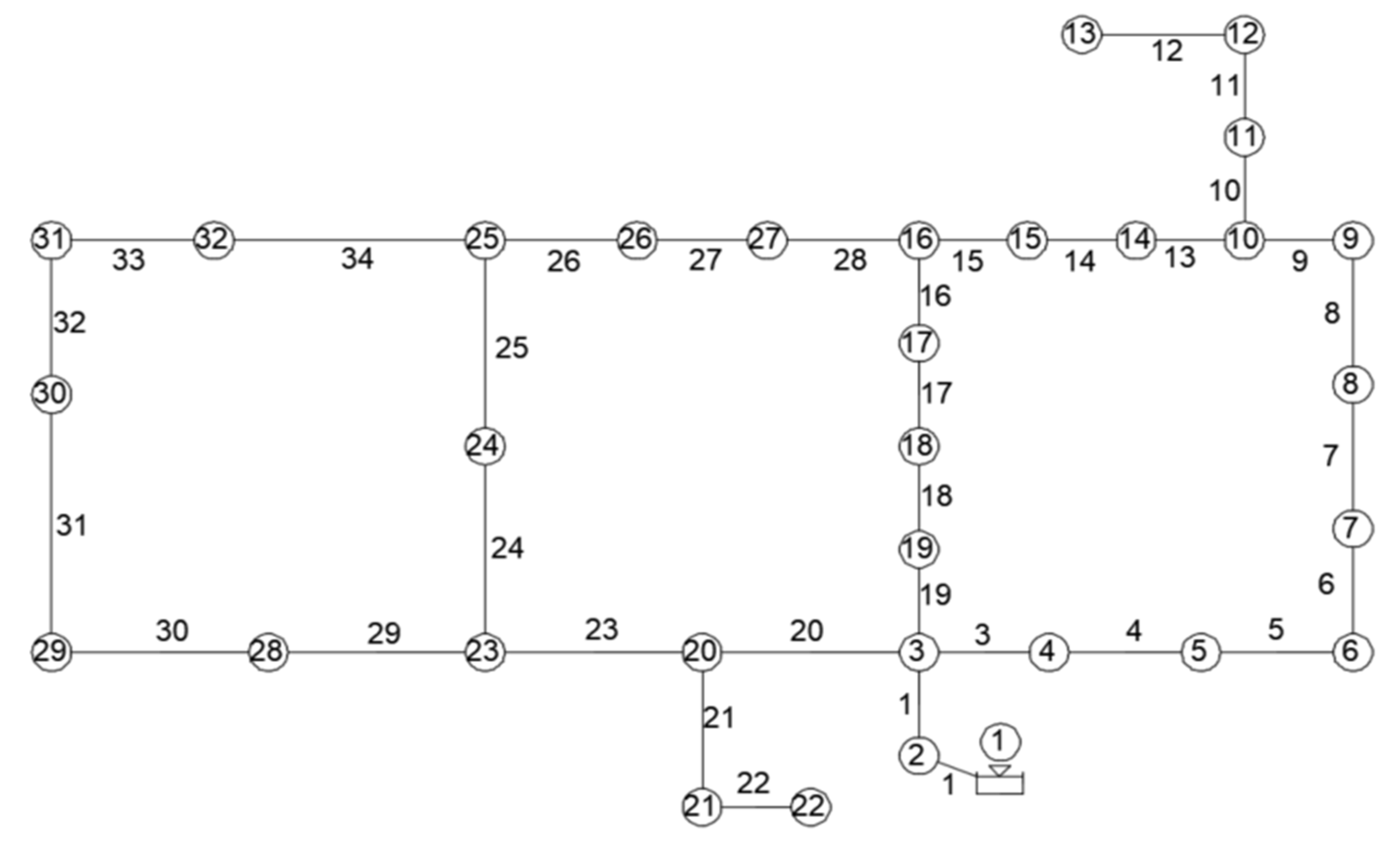
13]. They designed it for a problem without velocity restrictions and attempted to solve it using a variation of linear programming. Since then, it has been used in countless studies to test and evaluate new algorithms. Its data were provided by Alperovits and Shamir, and its layout is presented in
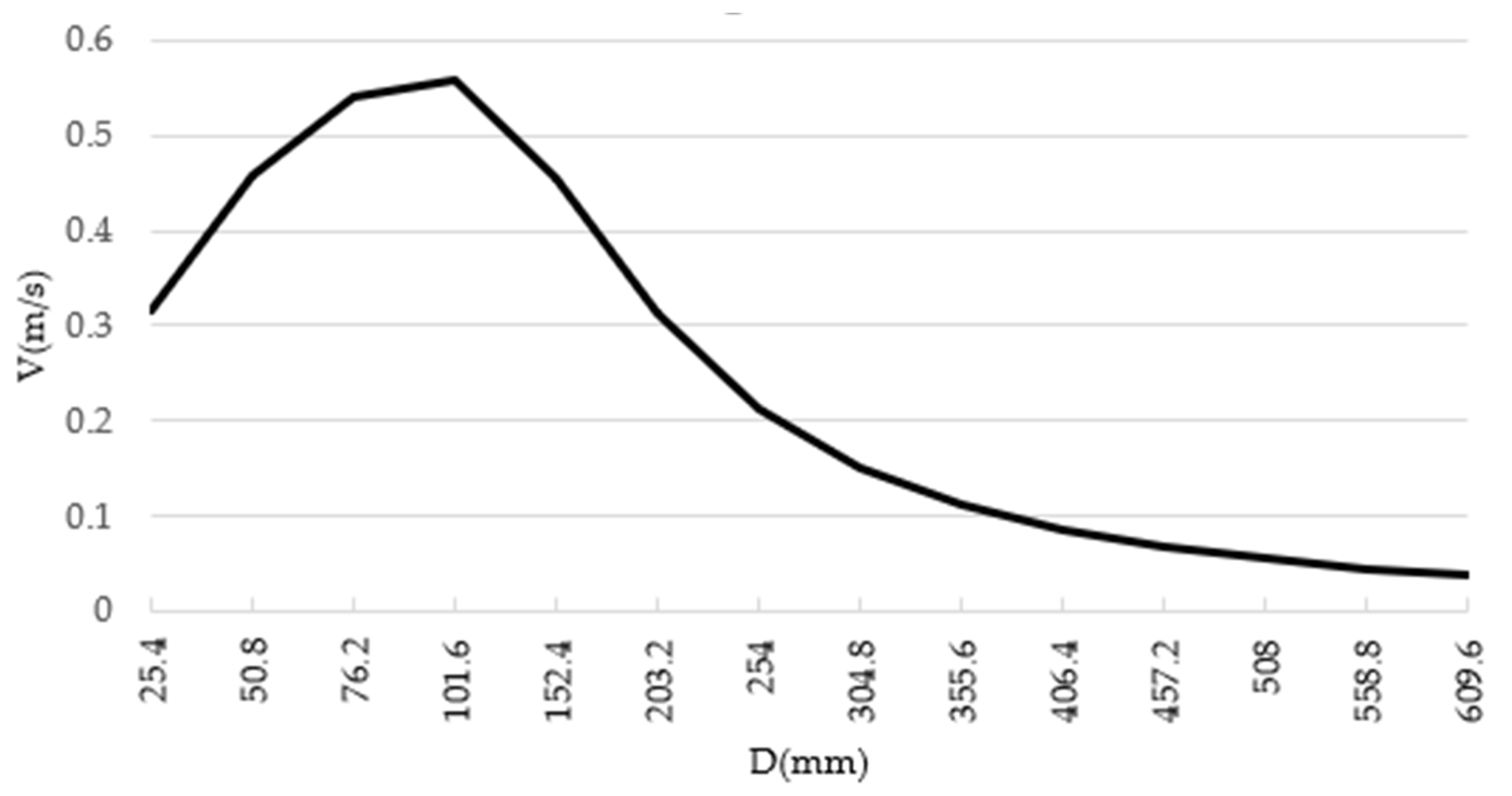
Figure 1. The optimum solution to this problem has already been found by many algorithms in the literature. It is given by the selection of diameters in mm: (457.2, 254, 406.4, 101.6, 406.4, 254, 254, and 25.4). In the course of a numerical experiment, let us vary the diameter of the last pipe over the whole range of available diameters, while keeping all the other diameters of the network constant. Then, a velocity versus diameter diagram can be created for the last pipe, such as the one in
Figure 2.
The shape of the curve in
Figure 2 above also appears when examining any other individual pipe in any looped network. The shape of the curve confirms that, generally, it is uncertain whether a pipe’s diameter should be increased or decreased in order to increase the flow velocity in the pipe. When trying to manipulate the flow velocities in the looped network, it should also be considered that changing the diameter of a pipe in a looped network will affect the velocities in all the other pipes in the network.
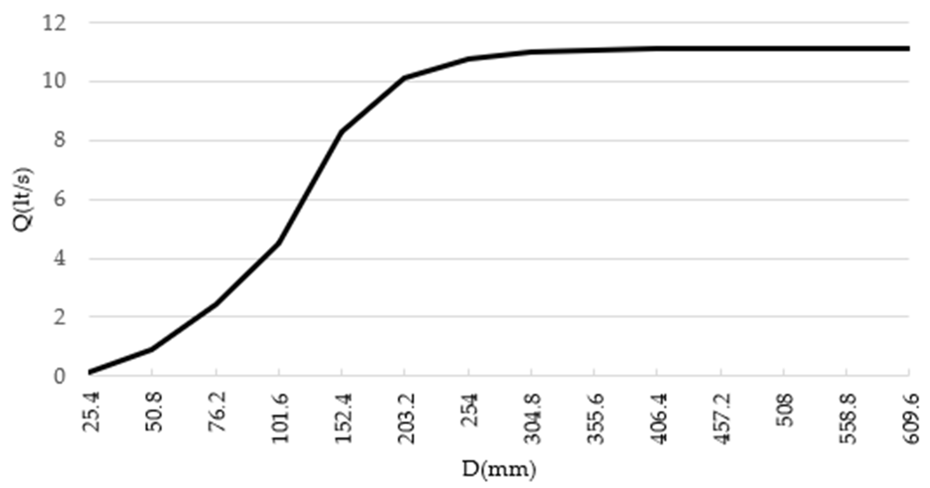
Figure 3 shows the change in the flow rate of the same pipe. Again, the shape of the curve is similar to any pipe in any looped network.
It can therefore be concluded that if the flow velocity in a pipe is out of allowable bounds, it is not certain whether decreasing or increasing its diameter will fix the problem. Furthermore, in some cases in which the pipe’s velocity is lower than the minimum, the problem may be impossible to solve with any diameter selection. This is because the maximum of the curve in
Figure 2 may be below the minimum velocity bound. A way to correct the velocity is to adjust the flow rate of the pipe by changing the diameters of the adjacent pipes. This will certainly lead to a desirable result. For example, if the flow rate of a pipe increases with an appropriate change in the diameter of an adjacent pipe, then it is certain that its flow velocity will also increase.
Stipanić et al. [
14] presented an interesting study showing the behavior of flow velocity in a network. Their research was not about optimizing the network from an economic point of view, but some of their conclusions were used in the present analysis. A section of a hypothetical water distribution network is presented in
Figure 4.
The cases analyzed below for adjusting flow rates and velocities can be applied respectively to any part of any looped network.
Figure 4 shows how the flow rate in pipe 1 can be increased. This can be done in five ways. The most obvious one is the increase in the diameter of pipe 1 itself, as can be seen in
Figure 3. Two others, according to the conservation of mass (Equation (2)) at node a, include:
In addition, the remaining two, according to the conservation of mass equation at node b, include:
These changes can also be applied to the sections of pipes connected to the pipes described above. For example, it has been mentioned that to increase the flow rate of pipe 1, the diameter of pipe 2 can be increased. Respectively, the diameter of any pipe upstream of pipe 2 can be increased with the same effect. The reverse changes have the opposite effect.
6. Targeted Path Search with Velocity Restrictions
The conclusions described above were incorporated in the original TPS algorithm in order to formulate a new, augmented targeted path search with velocity restrictions (TPSVR) algorithm.
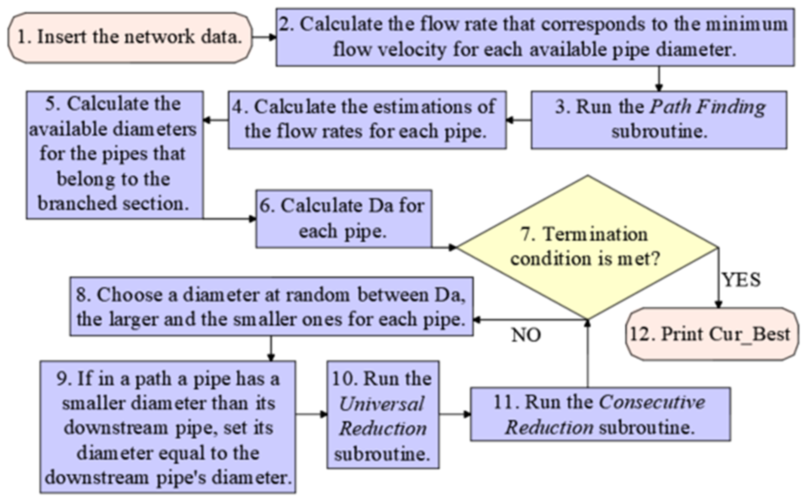
Figure 5 presents the flowchart of the TPSVR. The algorithm was guided by three subroutines, specifically the path finding, universal reduction, and consecutive reduction subroutines. The path finding subroutine remained the same as it is in the TPS algorithm. In the consecutive reduction subroutine, the only difference was that new solutions were only accepted if the velocity restrictions were not violated. Therefore, only the modified universal reduction subroutine was reanalyzed in the next subsection.
In Process 2 of the flowchart, the flow rate that corresponded to the minimum allowable flow velocity
was calculated, since it was used in the universal reduction subroutine. These flow rates were calculated for every commercially available diameter. Thus, the set
was obtained:
where
nav is the number of available diameters.
In Process 3 of the algorithm, the path finding subroutine was executed. Its purpose was to identify the most probable paths of water in the looped network. With that knowledge, the flow rates of the pipes could be estimated in Process 4. These were calculated by adding the flow rate of the downstream pipe to the demand of the downstream junction. If the network had branched sections, the flow rates of the pipes of these sections were the final ones. In the looped sections of the network, the flow rate of each pipe was estimated using the water flow paths that were derived from the path finding subroutine. When there were paths that ended in the same junction, the slope
was used to distribute the demand of the junction to each path:
Where
the hydraulic head in the supply junction
, and
is the total length of the path that connects s to the demand junction j. If, in the junction j with demand
, end n paths with slopes
, where
, then the pipes of each path
will also carry the following demand:
The addition of the velocity restriction constraint (5) to the classical optimization problem made it more difficult to solve it, as with any additional constraint. Nevertheless, there was an advantage that could be utilized. If the network had branched sections, it was possible to reduce the available diameters for the pipes of these sections. Since the flow rate of these pipes was known in advance from Process 4, it was easy to select as available only the diameters for which the water velocity would be within the predetermined limits. Solving the equation for D, substituting into Inequalities (5) and considering Equation (6), the minimum and maximum diameter of these pipes could be found. This advantage was not offered in the looped sections of the network, since the actual flow rates of the pipes were unknown. This was performed in Process 5 of the algorithm.
In Process 6, the initial diameters Da for all the pipes were assigned. Since the estimates of the flow rates of the pipes were calculated in Process 4, if a desired flow velocity was set, estimates of the diameters of the pipes could also be calculated. This flow velocity was set to 1 m/s, since this value is generally accepted as desirable in new networks. This value was chosen because it was about halfway through the velocity limits, and because it led to relatively small losses, since the head losses increased according to a power law as velocity increased. Therefore, if an initial velocity
Va = 1 m/s is assigned and if
Qai,
i = 1,2, …
np are the flow rate estimations that were calculated in Process 4, then the initial diameters will be:
Since continuous values for the diameters were calculated using Equation (14), these values were rounded to the closest available discrete value, according to the constraint (6). For each pipe, the available diameter that had the smallest difference from the diameter calculated by Equation (14) was selected.
The iterations of the algorithm began at Process 7 and continued until a user-defined termination criterion was met. At the beginning of each iteration, a “quasi-random” solution was generated in Process 8. For each pipe, a diameter was chosen randomly from Da, the smaller and the larger one, if of course, they existed in those available. At this point, there was a key difference compared to TPS. In the TPSVR, each iteration began with a new quasi-random solution that was optimized by the other subroutines; while in the TPS, the initial solution of the iteration was the currently best-found solution. This change was introduced because it was ascertained that the TPSVR showed an inability to escape from local optima in the previous design. By starting each iteration from a new quasi-random solution, the search expanded. At the same time, initializing from the diameters that were calculated by Equation (14), or diameters that were close to them, prevented a pointless search in areas of the search space where the objective function was highly infeasible.
This initial solution was “corrected” in Process 9, as is done in TPS. The difference here was that the solution was corrected within the iteration, as a new initial solution was created in each iteration. This solution was then optimized within the universal reduction and consecutive reduction subroutines. In the first iteration of the algorithm, the solution after its optimization was registered as Cur_Best. In each subsequent iteration, it was checked to determine if the resulting solution was better than Cur_Best, and if it was, it replaced it.
In the TPSVR, the knowledge of the paths of flow, or equivalently the direction of flow in each pipe in the network, was crucial. Based on this information, the flow velocities were regulated in the universal reduction subroutine. It was noted that the direction of flow could change with a different selection of diameters. For this reason, in each solution of the network, a new directed graph was created that showed the directions of flow resulting from the respective selection of diameters.
It should be noted that in the use of the TPSVR, the velocity constraints were treated as hard constraints, meaning that they were required to be absolutely satisfied. If the intention was to treat them as soft constraints, then the use of a penalty function would probably have been more efficient.
Universal Reduction Subroutine of the TPSVR
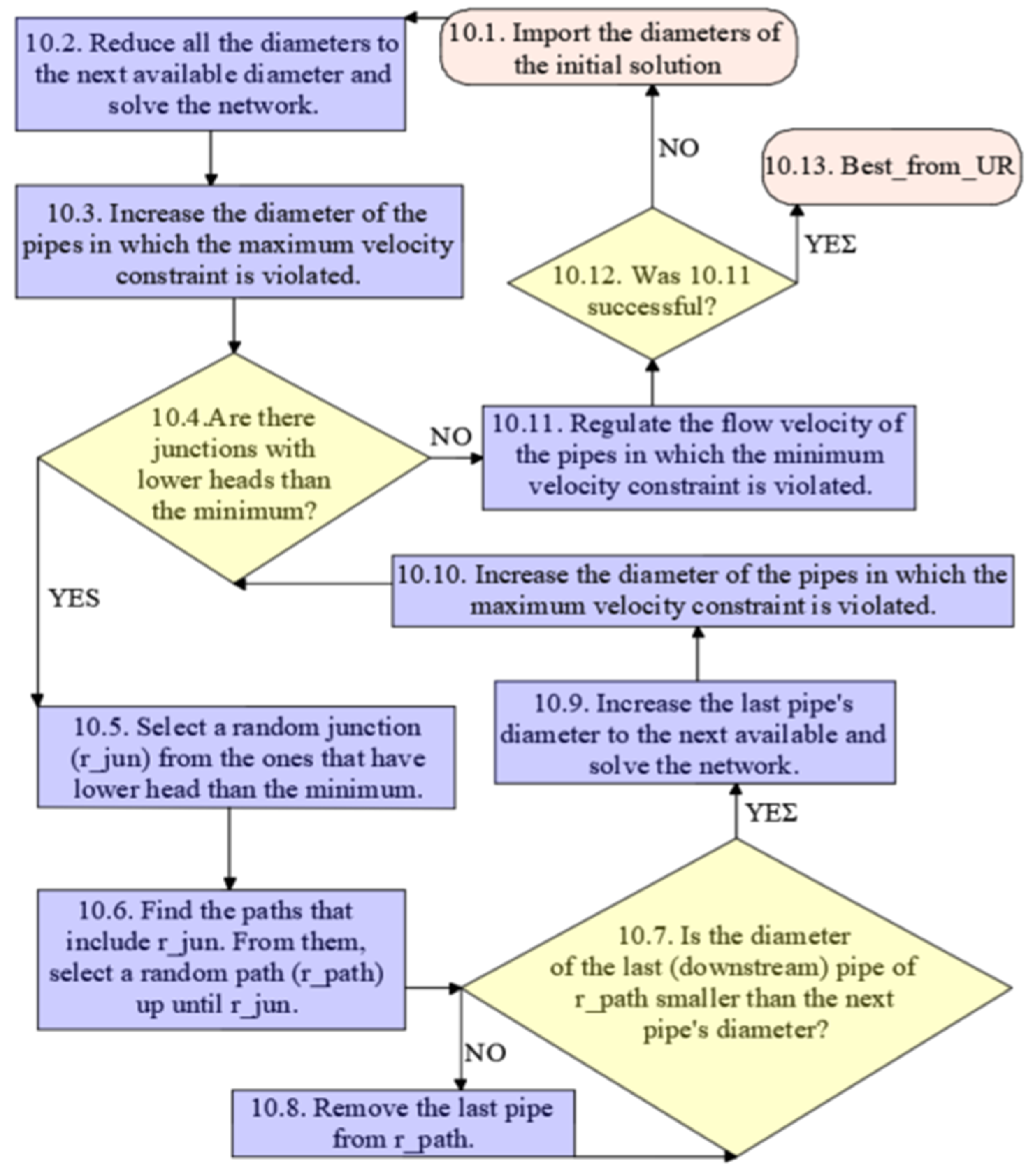
The mechanism that regulated the flow velocities in the network was incorporated in the universal reduction subroutine. The solution that was produced by Processes 8 and 9 given in
Figure 5 was initially imported into the subroutine.
Then, the procedure that followed can be described as follows in the form of a pseudocode and in
Figure 6 in the form of a flowchart.
The main purpose of universal reduction was to find an acceptable solution, and was not necessarily the best. Increasing the diameter at this stage helps the subsequent subroutine Processes to locate a solution that does not violate the minimum pressure constraints besides the velocity constraints. Let PH be the set of pipes in which the maximum velocity limit is violated. Process 10.3 is described by the following simple pseudocode.
While PH ≠ ∅:
- 1.1
Chose randomly a pipe p, p ∈ PH.
- 1.2
Increase the diameter of pipe p to the next available one.
- 1.3
Solve the network and update the set PH.
In processes 10.4–10.9, the minimum hydraulic head constraint was addressed, just as in TPS. In these, and specifically in 10.9, the diameters of the pipes always increased. However, there was a small chance that this would lead to a violation of the maximum velocity limit. This was explained by the shape of the curve in
Figure 2. Hence, Process 10.10 was added, which was similar to 10.3. When the programming loop 10.4–10.10 was completed, it was certain that the minimum pressure and the maximum velocity constraints were not violated. There were, however, pipes in which the minimum velocity constraint was violated.
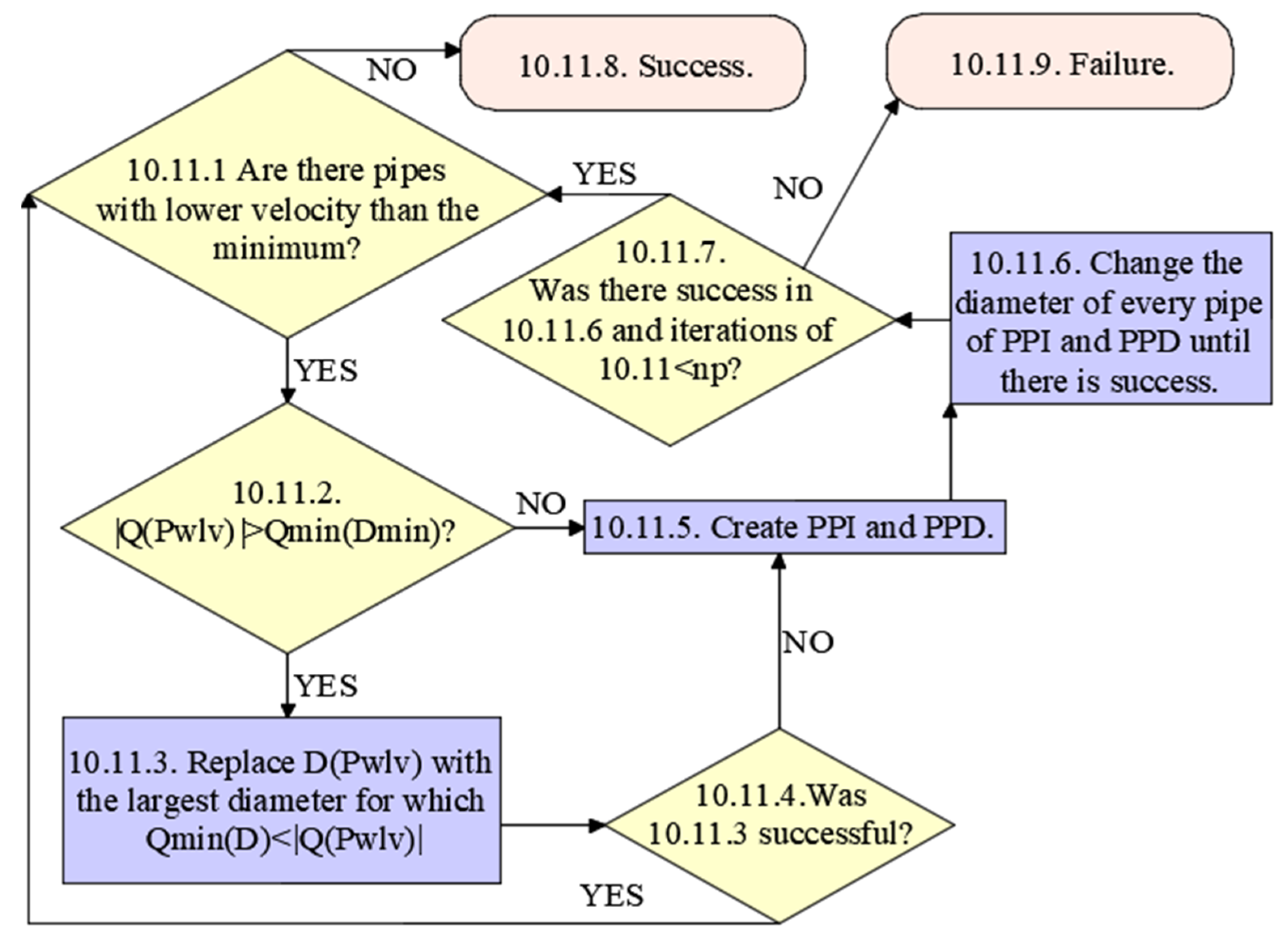
The minimum velocity constraint was addressed in Process 10.11, which was presented due to its size in the separate flowchart of
Figure 7. In Process 10.11.1, whether there were pipes in which the flow velocity was less than the minimum was checked. Of these, the pipe in which the flow velocity was the smallest is defined as the pipe with low velocity (Pwlv). In the other processes given in
Figure 7, we attempted to increase the flow velocity of only this specific pipe.
The process was iterative, and there was a limit to the number of iterations. This limit was set as equal to the number of pipes in the network (np), as it was proportional to the number of pipes in which the minimum velocity constraint could be violated. If this limit was exceeded, then the process had failed, and the algorithm returned to Process 10.1. It was also considered a failure not to find a solution that increased the velocity of Pwlv in one iteration, even slightly. This last feature was used as an escape route in case the algorithm stalled in an unfeasible solution from which a feasible one could not be obtained. The failure rate for all problems examined was less than 1%.
Figure 2 shows that there was a maximum flow velocity in one pipe while its diameter changed and the diameters of the other pipes were kept constant. This velocity may have been less than the minimum. Therefore, there may have been a situation in which the diameter of a pipe would fluctuate endlessly, without leading to a velocity higher than the allowed one. For this reason, a mechanism for monitoring each diameter change was introduced into the algorithm. If, in one iteration, the diameter of one pipe was reduced, in the next one it was not allowed to increase, and vice versa.
The Qmin was already calculated in Process 2 of the TPSVR, and consisted of the flow rates for each available diameter with which the minimum allowable velocity was achieved. In Process 10.11.2, it is checked whether the flow rate of Pwlv, |Q(Pwlv)|, was greater than the required flow rate to achieve the minimum velocity with the smallest available diameter, Qmin (Dmin). If this was the case, reducing the diameter of Pwlv would possibly increase its velocity. This was done in Process 10.11.3, and the selected diameter was the largest available diameter for which the minimum flow rate was less than the current flow rate of Pwlv. Process 10.11.3 is also described by the following pseudocode. Let Dav be the set of the available diameters, sorted in ascending order:
For every d of Dav:
- 1.1
If Qmin(d) < |Q(Pwlv)|:
- 1.2
Else:
Figure 7 and the above pseudocode show the absolute value of the flow rate |Q(Pwlv)|, considering that the flow rate had a negative value if the flow was in the opposite direction from what was initially set in the network. Process 10.11.3 was considered to have failed if one or more of the following applied after it:
The velocity of the Pwlv pipe had decreased;
There were junctions with lower hydraulic heads than the minimum;
There were pipes with a higher velocity than the maximum.
If none of the above was true, the process was considered successful, and the minimum velocity bound was rechecked. If the process failed, then the algorithm continued in Processes 10.11.5–10.11.8, with the aim to increase the flow in Pwlv.
In Process 10.11.5, two sets of pipes were created: the possible pipes increase (PPI) and the possible pipes decrease (PPD) sets. In these, the pipes that were candidates for a diameter increase or decrease were respectively stored. The PPI and PPD sets were created following the thoughts developed in
Section 5 and presented in
Figure 4. According to these, the following were placed in the PPI set:
The following were placed in the PPD set:
In all the looped networks, some pipes belonged to different paths. Therefore, these pipes may have been placed in both sets. However, the effects of changing the diameter of these pipes was uncertain. For this reason, these pipes were removed from both sets. Let us define the upstream and the downstream junction as up and down, respectively. The above can also be described by the following pseudocode.
For the Pwlv pipe itself, its flow rate was considered to determine in which set it would be placed. Thus, it was placed in the PPD set, if its flow rate was greater than the Qmin corresponding to the immediately smaller available diameter. Otherwise, it was placed in the PPI set in order to increase its flow rate by increasing its diameter.
The PPI and PPD sets were sorted so that the changes in diameters of specific pipes were tested first. The PPD set was sorted based on the proximity of each pipe to the Pwlv. Proximity here refers to how many junctions there were between the two pipes, and not their distance. The PPI set was sorted first based on the proximity of each pipe to its supply junction, and then based on its diameter. The reason was that generally, it was desirable to first increase the diameters of smaller pipes. If two pipes had the same diameter, then initially the diameter increase for the pipe that was upstream in its path would be tested. In that way, the general hydraulic requirement that the upstream pipes should have larger diameters than the downstream ones was met.
In Process 10.11.6. the changes in the diameters of the PPD and PPI sets were attempted until there was a success. As previously established, success meant increasing Pwlv’s flow velocity with a solution that did not violate the minimum pressure and maximum velocity constraints. However, the changes that were made to the pipes outside Pwlv now would certainly lead to an increase in the velocity of Pwlv. The process began by decreasing the diameter of the first pipe in the PPD set to the next available one. If the result was a failure, the diameter increase for the first pipe in the PPI set was attempted, then the diameter decrease for the second pipe in the PPD set, and so forth. Naturally, if a change in a diameter failed, the initial diameter was restored. If a change was successful, then the process stopped, and the algorithm returned to the evaluation of the velocity of the pipes (Process 10.11.1). If all possible changes failed, then Process 10.11 was considered to have failed, and the algorithm returned to the input of a new initial solution.
7. Application Example
For a better understanding of Process 10.11, an example based on the two-loop network was used. The layout of the network is presented in
Figure 1, in which the arrows show the flow direction for the diameters applied in the example. These flow directions were kept constant during the procedure. Obviously, this did not mean that these directions could not change with a different selection of diameters. In all the iterations of the example, pipe 8 was the Pwlv.
In the example in
Table 1, the flow velocity correction of pipe 8 was attempted, and was initially lower than the minimum (0.5 m/s). The process was successful since with the final selection of diameters, the flow velocity in pipe 8 was 0.56 m/s. In addition, the flow velocity bounds in the other pipes and the minimum pressure bound in any junction were not violated. In each iteration, it was checked whether the flow rate of pipe 8 was greater than the minimum flow results for the minimum available diameter. The minimum flow rates for each available diameter are presented in
Table 2.
Since, in this example, the flow rate of pipe 8 was greater in every iteration than the minimum results for the minimum diameter, in each iteration, the reduction in pipe’s 8 diameter was tested according to Process 10.11.3. If this failed, the PPD and PPI sets were created. According to
Figure 1, and because the flow direction does not change, in all iterations, it was PPD = {4, 7, 2} and PPI = {6, 5}. In the PPD set, pipes 4 and 7 were inserted before pipe 2, as they were closer to pipe 8. Pipe 4 was inserted before pipe 7 randomly, as their proximities to pipe 8 were the same. In the PPI set, pipe 6 was inserted before pipe 5 because it had a smaller diameter. Pipes 1 and 3 could be inserted in both sets as long as they led to both the upstream and downstream junction of pipe 8, and thus, they were not inserted in either.
If Process 10.11.3 failed, as in iteration 3, the following actions were performed with the following specific order until there was a success:
Reducing the diameter of pipe 4;
Increasing the diameter of pipe 6;
Reducing the diameter of pipe 7;
Increasing the diameter of pipe 5;
Reducing the diameter of pipe 2.
If an action failed, then the next diameter change was examined. If they all failed, then the entire process was considered to have failed, and the algorithm returned to the initial solution. The same was true if the number of iterations exceeded the number of the network pipes, which, in this example, was 8. It should be noted that the pipe with the lowest velocity (Pwlv) and the PPD and PPI sets were recalculated at each iteration, as they generally changed.
8. Applications of the TPSVR
The TPSVR was implemented in the same networks as the original TPS algorithm for better comparison. These were probably the most popular benchmark networks in the literature, specifically the two-loop, the Hanoi, and the Balerma networks. To test the efficiency of the TPSVR, a selection of the most popular optimization algorithms, along with TPS, were coded and applied to these networks with the velocity constraints of Equation (5). All the algorithms were coded in Python V3.6 and were executed on a personal HP laptop with an AMD 2.9 GHz processor. In all the applications, the minimum and maximum velocity were set as
and
. The penalty function that was used was that of Equation (10), with
. These algorithms are presented in
Table 3. They were coded according to the guidelines given by the authors of
Table 3 when they applied them to the problem without velocity restrictions. The parameters that were used were the ones that produced the best results according to the respective authors. Note that the TPSVR, as well as the TPS, did not require any parameters.
With the intention of testing the algorithms’ performances in different stages of their executions, three termination criteria were used for the first two networks, based on the maximum allowable function evaluation number (FEN). The FEN was set equal to 1000, 10,000 and 40,000. In the Balerma network, the FEN was set equal to 45,400, on one hand because smaller numbers were meaningless for such a large network, and on the other hand because this number was used extensively in the literature ([
19,
20] and others). The population sizes involved in the algorithms in
Table 1 were set at 50 for the first stopping criterion, and 100 for the second and third ones and for the Balerma network. The parameter
n1 of the SA algorithm was set equal to 70, 700, 200, and 3000 for the three criteria and for the Balerma network, respectively. Regarding the parameter p of the SCE algorithm, it was set equal to 2, 4, 5, and 5, respectively, for the same criteria and for the Balerma network.
Due to the stochastic nature of all the algorithms that were used, 20 independent runs of the programs were executed for each criterion and each algorithm. Nevertheless, independent runs did not make sense for the TPSVR, since in each iteration, the algorithm began from an independent random solution. In essence, whether there were five independent runs of 10 iterations or one of 50 iterations, it made no difference.
8.1. The Two-Loop Network
The layout of the network is presented in
Figure 1. The best value of the objective function to the problem without velocity restrictions was found to be 419,000 arbitrary monetary units. This was found by many different algorithms, so it was very probable that this was in fact the optimum. In this solution, the flow velocity in pipe 8 was 0.31 m/s, which was less than the minimum allowable (0.5 m/s), and therefore was infeasible for the problem with velocity restrictions.
The results of the 20 independent runs are presented in
Table 4, and they were very promising for the new algorithm. The best value of the objective function that was found was 426,000 arbitrary monetary units, which is presented in
Table 5. Interestingly, this solution had different diameters for several pipes compared to the corresponding best solution without velocity restrictions. That value was found by the TPSVR 2 times when the FEN was set equal to 1000, 12 times when it was equal to 10,000, and every time when it was set equal to 40,000. The fastest execution of the TPSVR in the ones for which the best value was found lasted 0.05 s and required 98 evaluations of the objective function. The slowest lasted for 18s and required 24,171 evaluations. When the results of the other algorithms were compared, the best performance found was that of the DE for the FEN of 10,000 and the FEN of 40,000. Regarding the performance of the TPS algorithm, it was evident that it provided good results for low values of the FEN, but it was unable to locate the best-found solution for higher values of the FEN. It is noted here that, as already stated, the TPS was enhanced by the inclusion of a penalty function.
8.2. The Hanoi Network
The Hanoi network was introduced by Fujiwara and Khang [
21], and also has been used extensively for the evaluation of new algorithms. The value of the objective function in the best-found solution without velocity restrictions was USD 6,081,128. It has also been found by many algorithms such as GA [
2], NLP-DE [
15], and others. In this solution, the flow velocity in pipes 1, 2, 3, 4, 17, 19, and 20 was higher than allowed; while in pipes 16, 28, and 31, it was lower. In fact, a solution with the specific velocity restrictions and the available diameters was impossible. This was due to the lack of available diameter to serve the flow rate of pipes 1 and 2 concerning the maximum velocity bounds. The flow rate of pipes 1 and 2 was constant and equal to 5.539 and 5.292 m
3/s, respectively. If the maximum available diameter of 1016 mm was selected for these pipes, the resulting velocities were 6.83 and 6.53 m/s, respectively. These velocities were much higher than the maximum allowed, which was 2.0 m/s. The layout of the network is presented in
Figure 8.
To enable the network to be solved with the specified velocity restrictions while keeping its other data identical, two new available diameters were added. These are 55 and 75 inches (in) or 1397 and 1905 millimeters (mm). In the Hanoi network, the cost of pipes in USD/m was set equal to
, where D is the diameter in inches. So, the corresponding costs of the two new diameters were USD 448.68 and USD 714.47/m, respectively. Practically, only the diameter of 75 inches was required for the network to be solvable. The 55-inch diameter was introduced into the problem for the sake of uniformity with the other available diameters. With a diameter of 75 inches, the flow velocities of pipes 1 and 2 were 1.94 and 1.86 m/s, respectively, so they were within the velocity bounds. The results of the tested algorithms are presented in
Table 6.
The good performance of the TPSVR was shown in this network as well, since it generally managed to find better solutions than the other algorithms. It was the only algorithm that managed to find reliable solutions, even when the FEN was set equal to 1000, while the other algorithms produced highly unfeasible ones. The SA and TPS, enhanced by a penalty function, also showed good performance in this problem. The best solution that was found is presented in
Table 7. The value of the objective function was USD 7,209,104.24. In this solution, the flow velocities varied between 0.58 and 2.00 m/s.
8.3. The Balerma Network
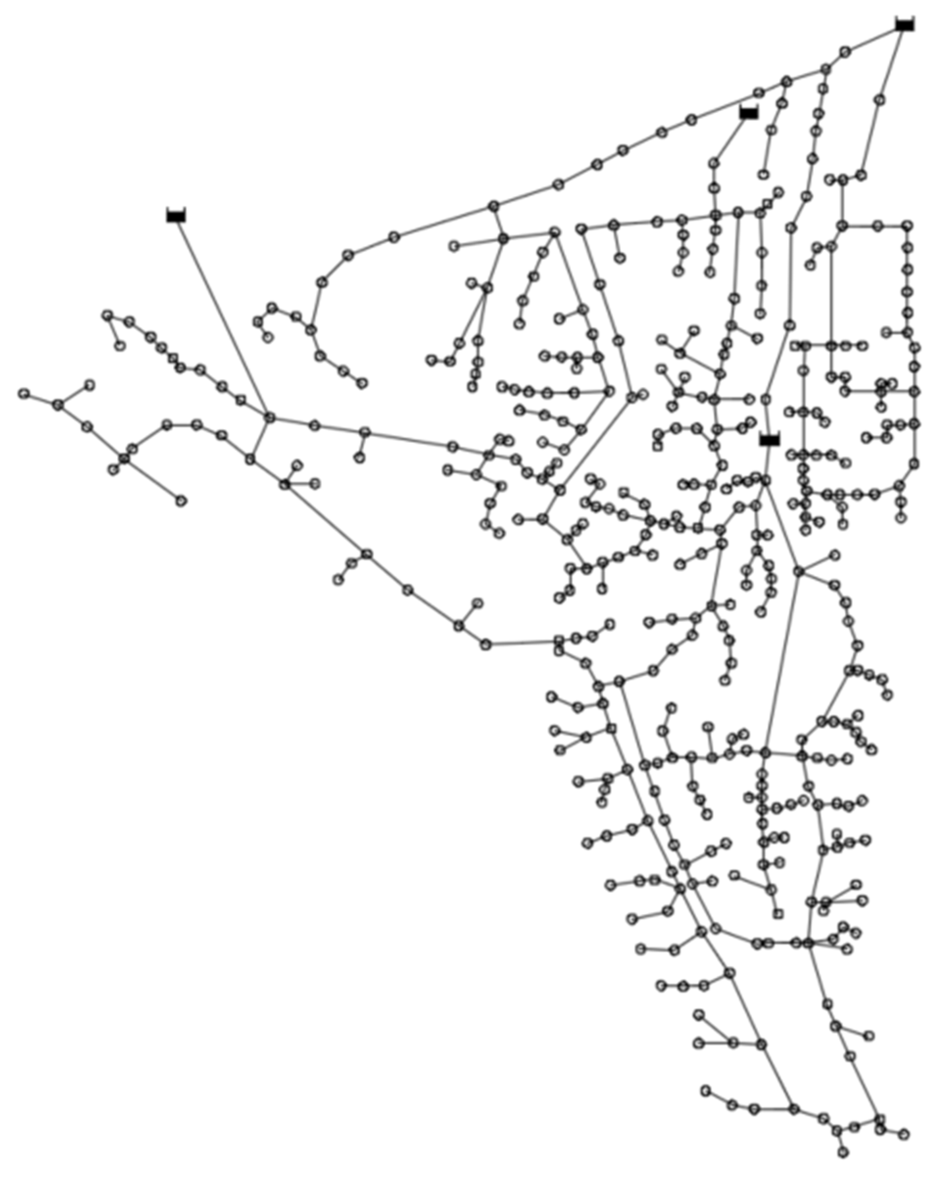
This network is an adaptation of a real water distribution network in the city of Balerma, located in the Andalusian region of Spain. Its layout is shown in
Figure 9. It was first presented by Reca and Martinez [
2], and various algorithms have been applied to it ever since. The authors also published the .inp file from EPANET, in which the network is presented in detail. In the best solution found by the TPS without velocity restrictions, the flow velocities of 48 pipes were higher than the maximum, and the flow velocities of 145 pipes were lower than the minimum. Since there were 454 pipes in the network, the flow velocities in 43% of the pipes were out of bounds.
As in the Hanoi network, the solution with velocity constraints and with the available diameters was impossible. In this network, diameters smaller than the available ones were also required. In order to solve the problem with velocity restrictions, we chose to include available diameters from 113 mm, which was the previous smallest available, down to 20 mm. The cost of each newly available diameter was chosen randomly, but followed the pricing logic of the originally available diameters. Additionally, a larger diameter than the existing ones was added. These are presented in
Table 8.
In a large network such as the Balerma network, it is possible to end up with small diameters for some pipes, as it resulted here, in order to enforce velocity restrictions. If these diameters are deemed unrealistic, there are some options available to the design engineer. One of them is to accept velocities lower than the minimum, in which case special attention should be paid to the consequent deposition of debris through regular supervision and maintenance. Another option is to locally modify the architecture of the network, and the proposed method is again suitable for this purpose. However, in this paper, adherence to the given architecture of the Balerma network was necessary in order to carry out the proper comparisons within the same framework employed for the previous unrestricted version.
The results of the application of the selected algorithms are presented in
Table 9. The good performance of the TPSVR in this difficult problem was obvious. Almost all the other algorithms, except for the SA, produced highly infeasible solutions. Another characteristic of the TPSVR that was evident in the results was its reliability, since the best and worst solutions had only a small difference. A table containing the optimal diameters resulting from TPSVR is given as
Table S1 in the Supplementary Material.


