Perspective

Past, Present, and Future of Using Neuro-Fuzzy Systems for Hydrological Modeling and Forecasting

1
Civil Engineering Discipline, School of Engineering, Monash University Malaysia, Subang Jaya 47500, Selangor, Malaysia
2
Future Building Initiative, Monash University, Melbourne, VIC 3145, Australia
*
Author to whom correspondence should be addressed.
Hydrology 2023, 10(2), 36; https://doi.org/10.3390/hydrology10020036
Submission received: 19 December 2022 / Revised: 23 January 2023 / Accepted: 24 January 2023 / Published: 26 January 2023
(This article belongs to the Special Issue Stochastic and Deterministic Modelling of Hydrologic Variables)

Abstract

:
Neuro-fuzzy systems (NFS), as part of artificial intelligence (AI) techniques, have become popular in modeling and forecasting applications in many fields in the past few decades. NFS are powerful tools for mapping complex associations between inputs and outputs by learning from available data. Therefore, such techniques have been found helpful for hydrological modeling and forecasting, including rainfall–runoff modeling, flood forecasting, rainfall prediction, water quality modeling, etc. Their performance has been compared with physically based models and data-driven techniques (e.g., regression-based methods, artificial neural networks, etc.), where NFS have been reported to be comparable, if not superior, to other models. Despite successful applications and increasing popularity, the development of NFS models is still challenging due to a number of limitations. This study reviews different types of NFS algorithms and discusses the typical challenges in developing NFS-based hydrological models. The challenges in developing NFS models are categorized under six topics: data pre-processing, input selection, training data selection, adaptability, interpretability, and model parameter optimization. At last, future directions for enhancing NFS models are discussed. This review–prospective article gives a helpful overview of the suitability of NFS techniques for various applications in hydrological modeling and forecasting while identifying research gaps for future studies in this area.

1. Introduction

Modeling hydrological processes has been challenging due to their high non-linearity, complexity, and being varied spatially and temporally [1]. The challenges are aggravated when dealing with sparse, missing, or poor-quality data. To date, many methods have been introduced and applied in hydrological modeling, mainly categorized into physically based and system-theoretic models. Physically based models have been widely used to simulate hydrological phenomena by approximating actual physical processes [2]. Despite their great capabilities, physically based models suffer from several factors, such as extreme computational effort, the need for many influencing factors, the imposed inaccuracies due to approximating several hydrological parameters, and the required prior knowledge. Therefore, developing a physically based model has always been challenging and time-consuming [3].
On the other hand, the system-theoretic (or data-driven) models have significant advantages over the physically based model in some cases. For example, unlike physically based models, data-driven models can directly map the associations between inputs and output without considering the physical process. As such, it is known to be more computationally efficient, less data-intensive, and less complex [4]. Linear or non-linear regression techniques such as autoregressive moving average (ARMA) and multiple linear regression (MLR) models are examples of such data-driven techniques. However, these techniques fall short when the model is challenged with extrapolation tasks since their prediction capacity is limited to what is learned from the calibration data [5]. Therefore, using a longer historical dataset for model calibration may make its predictability for unseen scenarios at the testing phase more reliable [6].
The need to improve the conventional data-driven models drove the motivation to introduce artificial intelligence (AI) and machine learning techniques into hydrological modeling. Despite sharing similar concepts of conventional data-driven models, AI-based techniques comprise considerably more advanced computational algorithms that do not require any prior specification of input–output associations [7]. AI techniques are known to excel in pattern recognition and handle many non-linear and non-stationary data adaptively, even if the data contain noises [5]. Using historical data as the input, AI-based models can capture the information precisely without compromising prediction accuracy, yet at a lower computation cost, complexity, and time. The artificial neural network (ANN) is one of the well-known AI-based algorithms used in engineering applications, including hydrological modeling. An ANN comprises a network of human brain-inspired processing nodes known as neurons. These neurons appear in different layers and are interconnected using links with associated weights. This network can identify relationships between inputs and outputs through an iterative learning process from the training dataset. So far, several learning algorithms have been proposed for training an ANN. Despite their successful usage in different modeling applications, ANNs suffer from several issues, such as a lack of transparency, making them black-box models [8]. This shortcoming became a motivation to enhance an ANN’s transparency by integrating fuzzy logic into its learning process, producing a new family of AI-based techniques known as neuro-fuzzy systems (NFS), which can be called grey-box models [4].
NFS combine the connectionist structure of an ANN and the reasoning skills of fuzzy logic to map complex associations between inputs and outputs. The fuzzy inference system (FIS) embedded in NFS allows them to describe the relationships between inputs and outputs in a series of fuzzy IF–THEN rules. Fuzzy logic is the backbone of fuzzy rules in NFS and offers approximate reasoning using fuzzy values. While retaining the strength of a typical ANN, NFS offer a more transparent structure that allows the physical interpretation of the problem to some extent. There are two classes of FISs, which are called linguistic and precise. In a linguistic FIS, the antecedent and consequent rules are defined using fuzzy sets. The Mamdani FIS [9] is the most well-known linguistic FIS that is widely used in several applications. The Mamdani-FIS tends to be computationally intensive, but it is effective in classification problems. On the other hand, in a precise FIS, only the antecedent rules are defined using fuzzy sets, while the rules in the consequent comprise weighted linear functions of crisp input data. The Takagi–Sugeno FIS [10] is the most widely-used precise FIS since it is computationally less complex and is particularly favorable when numerical outputs are desired.
NFS techniques gained popularity among researchers in the early 2000s and have been used for many hydrological modeling and forecasting applications since then. The early applications of NFS in hydrological modeling were by Gautam and Holz [11] and Gautam, Holz [12], focusing on rainfall–runoff modeling and water level forecasting, respectively. Since then, NFS algorithms have been widely used in different applications in hydrology, including rainfall–runoff modeling [13,14,15], rainfall forecasting [16,17,18], streamflow forecasting [19,20,21,22], groundwater level modeling [23,24,25], evaporation and evapotranspiration modeling [26,27,28,29], water quality modeling [30,31,32,33], sediment transport modeling [34,35,36], etc.
Despite the successful usage of NFS in a wide range of applications in hydrology, several challenges and shortcomings are reported in the literature that need a critical review. For example, input selection is an essential stage in NFS model development where the model performance can be significantly jeopardized by selecting the wrong choices. Similarly, choosing the right dataset for training the model impacts the model’s performance during validation. Moreover, the model’s adaptability to climate change or urbanization depends on its learning algorithm. In addition, the transparency of the model depends on the adopted FIS in its structure. As can be seen, depending on the hydrological problem, the requirements for model development could be different. Therefore, it is necessary to properly understand each hydrological problem’s needs to choose the right NFS algorithm and data. The presented work aims to address this research gap through three stages. Firstly, this perspective study reviews the NFS structure and learning system fundamentals. In the next phase, this article discusses the challenges in developing hydrological models using NFS and reviews the published efforts in addressing them. In the end, potential future studies or research directions to further enhance the NFS-based hydrological models are presented.

2. Neuro-Fuzzy Systems

2.1. Fuzzy Inference System

A fuzzy inference system (FIS) consists of (1) a fuzzification layer that transforms crisp input values into fuzzy ones, (2) an inference layer that utilizes a set of fuzzy rules to perform inference operations, (3) a rule-based containing set of fuzzy rules which is determined by a membership function, and (4) a defuzzification layer that transforms fuzzy values to crisp ones as the output of the system, as shown in Figure 1.
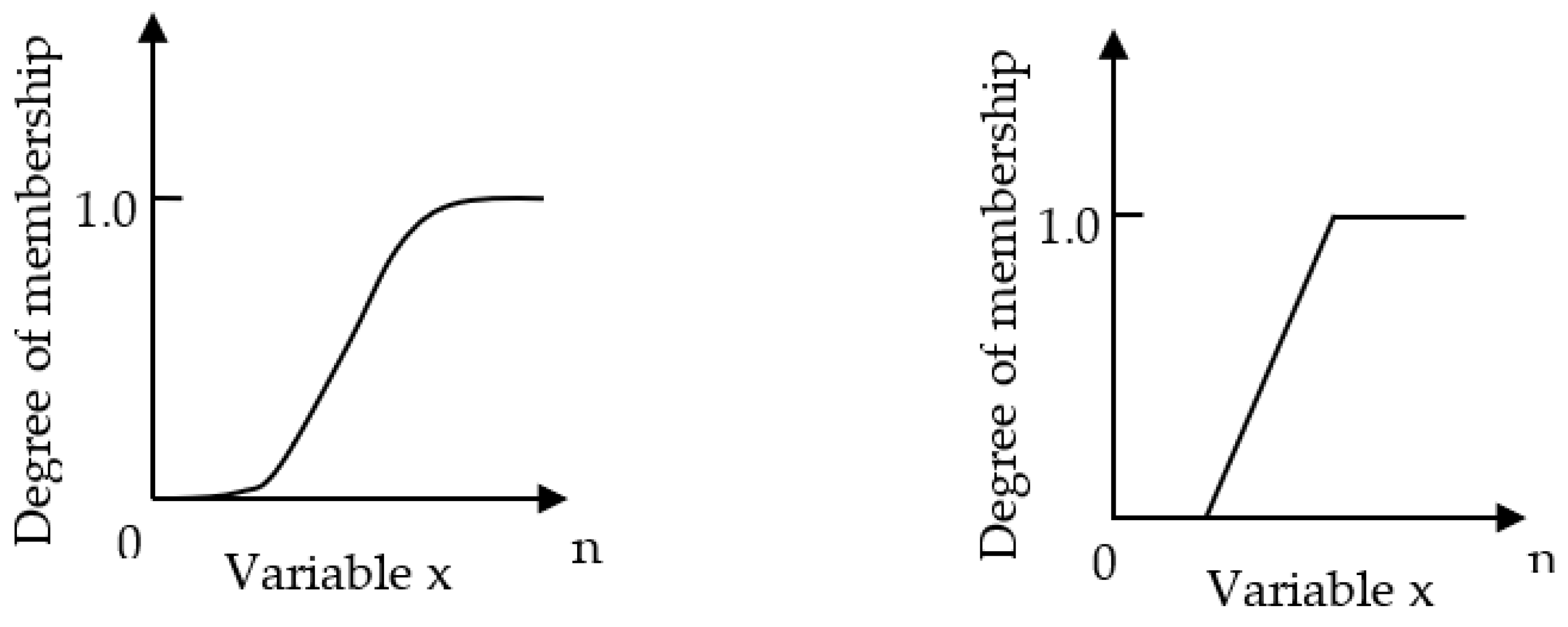
The fuzzy membership function determines the fuzzy logic in the fuzzy rule base. Fuzzy logic is multivalued and deals with degrees of membership and truth. Its value typically ranges from 0 (zero membership/false) to 1 (full membership/true). There are two typical membership functions: smooth curve and linear piecewise function, as shown in Figure 2. The well-known membership functions are triangular, trapezoidal, Gaussian, and sigmoidal [37].
The general structure of fuzzy IF–THEN rules is defined as:
IF X is xm, THEN Y is ym
The IF and THEN statements are known as “antecedent” and “consequent”, respectively. In this rule, X and Y are the input and output variables, respectively, while xm and ym are specific values of those variables. The rule antecedent is determined by a predefined membership function used to partition the input space. However, the rule structure differs based on the type of FIS used in the model (e.g., Mamdani or Takagi–Sugeno).
In Mamdani FIS, both rule antecedents and consequents are determined by fuzzy sets as shown in Equations (2) and (3):
Rule 1: If x is A1 and y is B1, then Z1 is C1
Rule 2: If x is A2 and y is B2, then Z2 is C2
where A and B are membership values for input variables x and y, respectively; and C is the membership value of output variable Z.
On the other hand, in the Takagi–Sugeno FIS, the rule antecedent is defined by fuzzy sets, while the consequent is typically a linear function, as shown in Equations (4) and (5):
Rule 1: If x is A1 and y is B1, then Z1 = p1x + p2y + p3
Rule 1: If x is A2 and y is B2, then Z2 = q1x + q2y + q3
where p1, p2, p3 and q1, q2, q3 are the parameters of output functions Z1 and Z2, respectively.

2.2. Types of Neuro-Fuzzy Systems

The NFS algorithms can be categorized into three major types based on their functionality and structure, as follows:

2.2.1. Cooperative Neuro-Fuzzy Systems

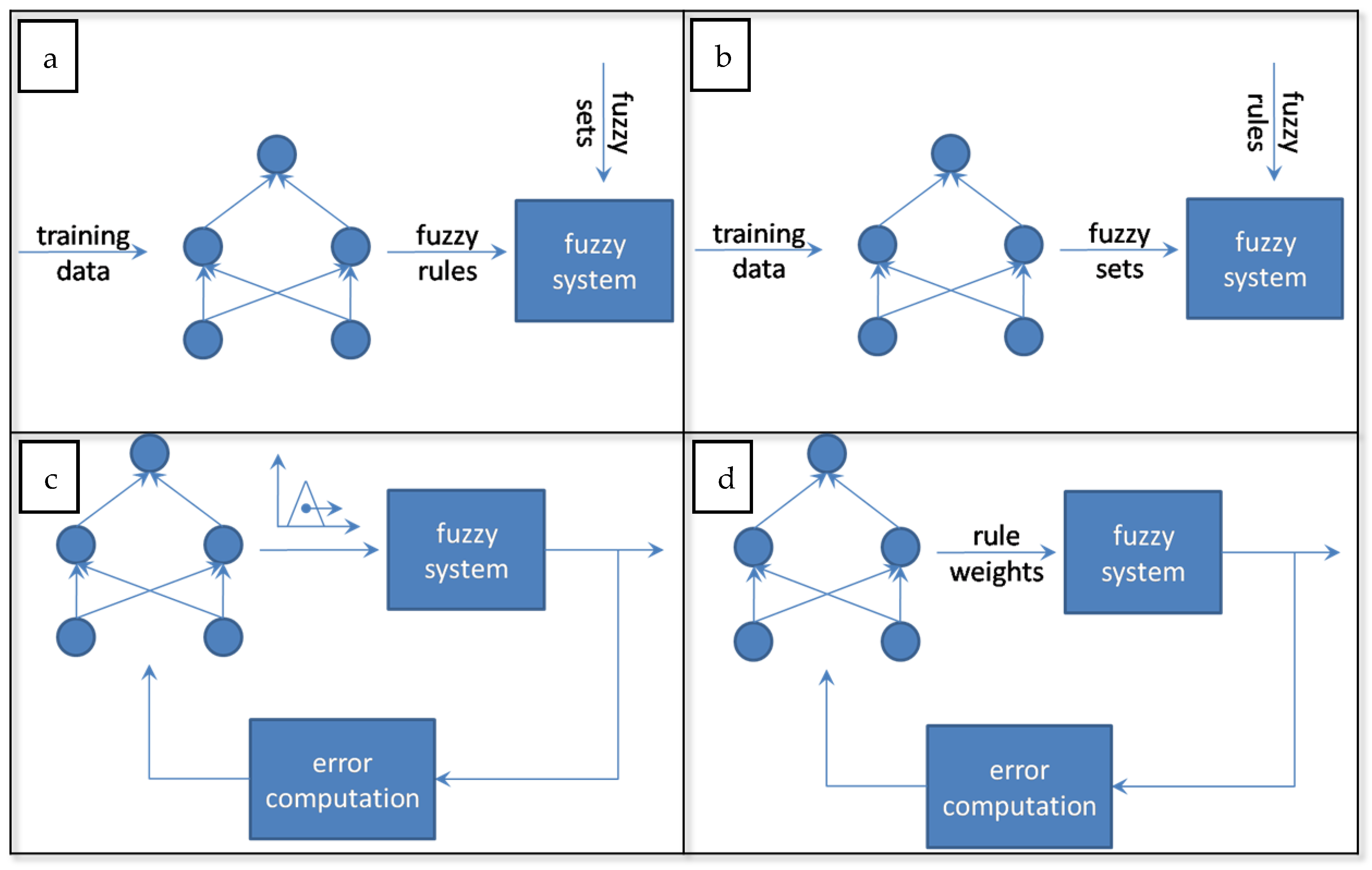
In cooperative NFS, ANNs and FISs operate independently at different phases. The ANN is tasked with identifying the parameters and initializing the FIS, which can be performed online or offline. Subsequently, the ANN task is completed, and the FIS will carry out its operation to determine the output. This type of NFS suffers from interpretability issues, and the complete integration of the ANN and FIS is not achieved at its full potential. Figure 3 shows four types of cooperative NFS algorithms [38]. Type 1 cooperative NFS use the ANN to define fuzzy rules from the training dataset with fuzzy systems receiving predefined fuzzy sets. A type 2 cooperative NFS has its fuzzy rules determined through membership functions using a set of training data prior to the initialization of the fuzzy system, which is then combined with a predefined set of fuzzy rules. Both type 1 and type 2 implement an offline learning approach. In type 3 cooperative NFS, the ANN implements the online learning of membership function parameters to update the fuzzy system. However, the initial fuzzy rules and membership functions must be specified. Finally, in type 4 cooperative NFS, the ANN determines the weight for each fuzzy rule which can be performed online or offline, directly influencing the importance of each fuzzy rule in the fuzzy system.

2.2.2. Concurrent Neuro-Fuzzy Systems

Concurrent neuro-fuzzy systems work by having the ANN pre-process the input or post-process the output of fuzzy systems [38]. The main drawback of this type of NFS is that the results are not entirely interpretable, and the ANN does not introduce changes to the structure of fuzzy systems.

2.2.3. Hybrid Neuro-Fuzzy Systems

In hybrid neuro-fuzzy systems, the integration of the ANN and FIS is achieved appropriately. Both AI tools operate efficiently as one entity. The ANN provides the learning algorithm and trains the model using historical data. Furthermore, the ANN optimizes the parameters of the fuzzy system. The human-inspired approximate reasoning of the FIS is then adopted to employ fuzzy rules in predicting the results [38]. The training of such models can be carried out either online or offline, which is thoroughly discussed in Section 3.4. Depending on the FIS type used in their algorithm, hybrid NFS can be a linguistic (or Mamdani) or precise (or Takagi–Sugeno) type. A linguistic hybrid NFS, which uses Mamdani FIS, generates the linguistic output from a set of linguistic input variables. It is particularly favorable when a linguistic output is desired; therefore, providing a clear interpretation of the physical process (e.g., a hydrological process) is achievable. Some examples of well-known linguistic hybrid NFS are the fuzzy adaptive learning control network (FALCON) [39] and the neuro-fuzzy control (NEFCON) [40]. In contrast, precise hybrid NFS generate a crisp output using fuzzy inputs. The main difference between various precise hybrid NFS is their learning process which can be local or global. The most widely used precise hybrid NFS in hydrological modeling is the adaptive network-based fuzzy inference system (ANFIS) [37].
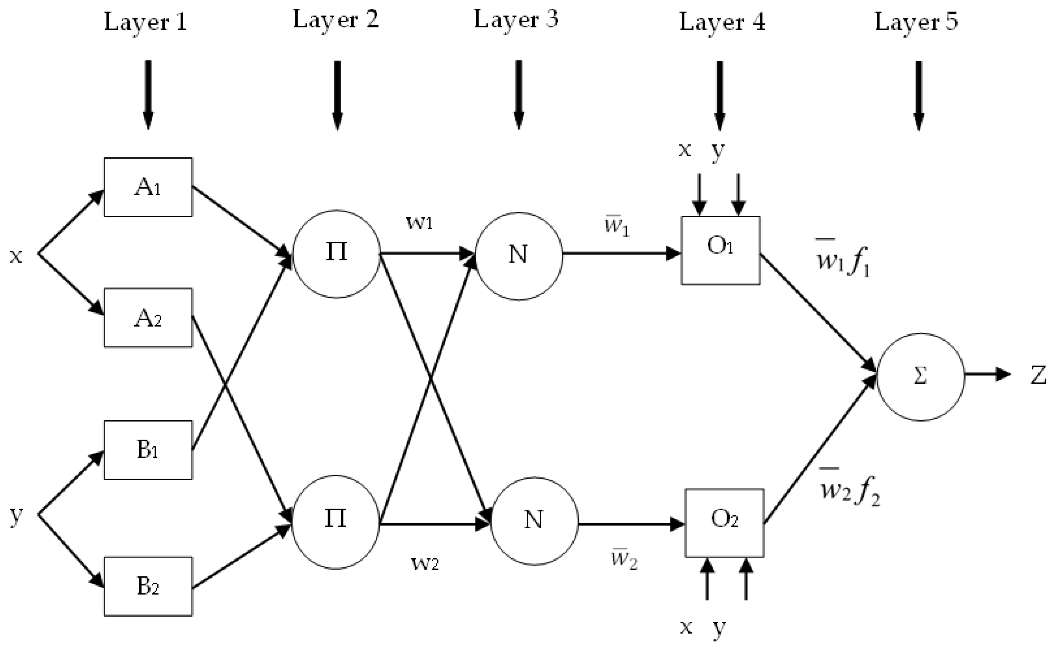
An ANFIS employs a Takagi–Sugeno FIS, and its structure comprises five layers, as illustrated in Figure 4. The nodes in Layer 1 generate the fuzzy membership values for each input variable using a defined membership function. The nodes in Layer 2 (shown by ∏) multiply the incoming signals from Layer 1 and calculate the firing strength for each rule. The nodes in Layer 3 (shown by N) normalize the firing strength received from Layer 2. In Layer 4, each node (shown by O) is responsible for calculating the contribution of one of the model rules using the first-order linear Takagi–Sugeno output function. Lastly, the single node in Layer 5 (shown by Ʃ) calculates the weighted global output (shown by Z). Further details of each layer operation can be found in Talei, Chua [41].
An ANFIS uses the back-propagation (BP) algorithm to modify the initially chosen membership functions, while the least mean square (LMS) algorithm is used to determine the coefficients of the linear output functions. An ANFIS has global learning, meaning that the parameters of the fuzzy system are optimized offline during the training process and stay fixed during testing. NFS models with global learning are incapable of being used in real-time applications and are more sensitive to noise (Hong and White, 2009).

3. Challenges in Developing NFS-Based Hydrological Models

3.1. Data Pre-Processing

Data pre-processing is one of the most important steps in developing a hydrological model before utilizing the data. Hydrological data often contain noises and drastic fluctuations. Several pre-processing approaches have been practiced to deal with such issues. For example, to assess the data’s homogeneity, a double mass analysis can be conducted, while the Mackus test [42] can be used to evaluate the data sufficiency [43]. Data standardization is one of the standard data transformation methods used to modify the data distribution by scaling the data into a specific range. Past studies suggested that standardization is necessary for data-driven techniques and improves performance [44]. Furthermore, it helps to remove periodicity present in data [45]. For ANNs, however, values close to 0 and 1 need to be avoided during standardization due to the sensitivity of the neurons’ activation functions to such values [8]. Although standardization improves an NFS model’s performance, sensitivity to values close to 0 and 1 is reported. Data standardization for developing NFS-based hydrological models is well-practiced [43,45,46,47,48]. One of the common standardization methods is a linear transformation [49]. Aqil, Kita [50] applied a log transformation to the data to achieve faster convergence. The model achieved better performance, but it was reported that the effect of such a transformation diminished as the network sizes increased.
In recent years, many studies have integrated NFS with a wavelet transformation as a data pre-processing technique to achieve better performance. Wavelet transformation is a signal processing technique that decomposes original time series into different frequency levels for further analysis. This method captures information at different resolution levels [51], assessing the temporal variation of the time series [52] and denoising them [53,54,55]. Shabri [56] used different types of the wavelet transform, including continuous wavelet transform (CWT) and discrete wavelet transform (DWT), where the latter is more suitable for forecasting applications due to its lesser computation time. DWTs commonly operate at two sets of function, high pass and low pass, which decompose the time series to one comprising its trend (approximation) and another comprising high frequency (details) [57]. There are several types of mother wavelets which implement the wavelet transforms such as Daubachies (Db), Haar (Ha), Symmlet (Symm), Coiflet, Mexican Hat, and Morlet wavelets.
Shabri [56] developed a wavelet-couple ANFIS model (WANFIS) to estimate monthly SPI as a drought indicator, which showed more accurate results than the ARIMA and conventional ANFIS model. Sehgal, Sahay [58] investigated the effect of using all wavelet components (denoted as WANFIS-SD) and ignoring noise wavelet components by only utilizing the effective components (denoted as WANFIS-MS), where the former showed better performance at high flood level forecasting. In a daily water level forecasting application, Seo, Kim [59] used the WANFIS with a Symmlet mother wavelet of order 10 (WANFIS-symm10) and yielded the best performance among other models. Barzegar, Adamowski [52] assessed different types of mother wavelets (Db, Symm, Ha) coupled with an ANN and ANFIS at three levels in which the WANFIS with a Db4 mother wavelet decomposition showed the best performance in water salinity modeling. Nourani, Alami [60] integrated a self-organizing map (SOM) as a spatial pre-processor and DWT as a temporal data pre-processor alongside wavelet transform coherence (WTC) for input selection to infill and model groundwater level data. Moreover, a DWT can also be used to denoise the time series where, coupled with generated jittered data, it shows significant improvement in performance due to the robust identification of hidden trends in the data (Nourani and Partoviyan [61]). Abda and Chettih [62] highlighted the superiority of wavelet transform coupled with an ANFIS and ANN compared to the Hilbert–Huang transform in daily flow rate forecasting.

3.2. Input Selection

The type and number of inputs used in NFS models ultimately contribute to establishing the model structure. The number of fuzzy rules in the rule base increases exponentially with the increasing number of inputs, which may unnecessarily increase the model’s complexity [4]. Challenges related to data availability may also encourage the usage of fewer input variables. Therefore, employing appropriate methods in input selection undoubtedly becomes important when developing NFS-based hydrological models. It is worth noting that introducing new inputs without a proper understanding of hydrological processes may adversely affect model performance. Therefore, before applying any input selection technique, it is necessary to have a list of hydrologically sound input candidates that could be informative in predicting the desired output. For instance, Chang and Chang [63] introduced the human-controlled reservoir outflow as an input for predicting reservoir water levels. Esmaeelzadeh, Adib [64] used snow-covered areas extracted from satellite images as inputs for developing a long-term seasonal streamflow forecasting model alongside other standard input variables. Adnan, Liang [19] considered the calendar month number as the input to factor in the periodicity in streamflow forecasting. Ali, Deo [65] and Lohani, Kumar [66] adopted a similar approach for drought forecasting and monthly reservoir inflow prediction, respectively.
NFS have been commonly used to develop multiple input single output (MISO) models, where several combinations of inputs can be formed. Perhaps the most basic approach for input selection is through sensitivity analysis, which systematically checks the importance of input candidates in a model. The trial-and-error-based approach has been used in several NFS-based hydrological modeling applications, such as evapotranspiration modeling [67] and groundwater forecasting [45]. While it is common to use the trial-and-error method by testing out different combinations of inputs, employing proper techniques may save time and effort by narrowing down the candidate list to the most influential and informative inputs in predicting the desired output. For example, the Gamma test is a non-parametric input selection technique that finds a set of suitable input candidates by minimizing the mean squared error (MSE) [68]. This method can suggest the degree of model complexity using the selected inputs. The Gamma test has been used for input selection in several NFS-based hydrological modeling applications, including evaporation estimation [69,70], modeling suspended sediment concentration [71], and daily river flow simulation [72].
The other well-known input selection approach is the principal component analysis (PCA) which identifies the linear correlation between input variables aiming to reduce data dimensionality. It assists input selection by avoiding redundancy and generating a new set of variables known as principal components from the original dataset. PCA has shown successful application with NFS in reducing the number of inputs. For example, in a water quality modeling application to simulate chemical oxygen demand (COD) and suspended solids, Wan, Huang [73] used PCA to reduce the number of potential inputs from six to four. Civelekoglu, Perendeci [74] employed PCA to reduce the input variables in an ANFIS model from eight to four and eleven to nine for modeling the COD and total nitrogen, respectively. In a separate study, Civelekoglu, Yigit [75] narrowed down the potential input candidates into three principal components in modeling the COD. Parsaie and Haghiabi [76] used PCA to identify the Froude number and ratio of weir height to upstream flow depth as the most influential parameters for estimating the discharge coefficient using an ANFIS model. Bartoletti, Casagli [13] confirmed the superiority of PCA over the Thiessen polygon method with GIS when coupled with an ANFIS in rainfall–runoff modeling; the authors concluded that using PCA could offer less algorithmic complexity and improved accuracy in the model.
One of the widely-used input selection techniques is correlation analysis. In this approach, a high correlation between an input candidate and the desired output will be the selection criterion. The correlation analysis can be conducted using three different functions named the autocorrelation function (ACF), the partial autocorrelation function (PACF), and the cross-correlation function (CCF). The ACF can identify the most correlated output antecedent with the output. For example, the discharge antecedent Q(t − 1) may be selected by the ACF as one of the informative inputs in predicting discharge at the present time, Q(t). On the other hand, one or a few rainfall antecedents could be selected as inputs by the CCF to predict runoff. The correlation analysis has been used in different NFS-based hydrological modeling applications, including rainfall–runoff modeling [77,78], groundwater modeling [79], water level forecasting [80], flood forecasting [81,82], evapotranspiration modeling [83], and El Niño Southern Oscillation (ENSO) forecasting [84]. In all reviewed studies that used correlation analysis, the inputs with a cross-correlation coefficient (CC) above 0.5 are considered potentially strong candidates, with a CC between 0.6 to 0.8 for the selected influential ones. On the other hand, the autocorrelation coefficients are generally high for the first one or two output antecedents, and they drop drastically by increasing the lead time. Therefore, it is common to use the first output antecedent as one of the strong input candidates in NFS-based hydrological models. In a novel approach, correlation analysis can be integrated into mutual information analysis to avoid selecting those highly correlated inputs that share mutual information with the output [85,86]. This minimizes redundant information being fed to the model.
In summary, any of the techniques mentioned earlier can be used for input selection in NFS-based hydrological models. However, a sensitivity analysis may still be needed to choose the most informative but trimmed input combination to avoid unnecessary model complexity. In most NFS algorithms, the users need to predefine the number of membership functions (fuzzy labels), which along with the number of inputs, govern the number of generated fuzzy rules. For example, in an ANFIS model with n inputs and m membership functions, mn rules are expected to be generated. As can be seen, the number of inputs can increase the number of rules exponentially. Therefore, it is good to avoid adding those inputs that do not improve the model performance significantly, as they may slow down the model.

3.3. Training Data Selection

In most of the hydrological models, using a continuous time series is expected. However, event-based modeling is also used in some applications, such as rainfall–runoff modeling. One of the main challenges in both approaches is choosing suitable training and validation datasets to calibrate the model before being tested by an unseen dataset [82].

3.3.1. Continuous Time Series Modeling

In continuous time series modeling, more than 60% of the available data is typically suggested for training, while the remaining data is left for testing purposes. The training dataset contributes to the model calibration and makes it ready to be tested for an unseen dataset (i.e., the testing dataset). This ensures that the dataset used to train the model covers all the characteristics of the hydrological problem to obtain a reliable and effective prediction [87]. Perhaps the most common approach for selecting the training–testing datasets is to split the data in chronological order. To avoid any biasness, it is recommended to split the data so that the statistical characteristics of the two datasets (i.e., average, standard deviation, etc.) remain relatively close. Moreover, the training dataset needs to contain sufficient extreme (critical) events to help the model perform well in the testing dataset [88]. Randomizing the dataset for the training and testing datasets is another common approach; however, it may introduce risk whereby training data do not cover the characteristic of the problem. As such, a k-fold cross-validation method that allows different segments of the datasets being used for training and testing is recommended. Cross-validation helps to identify training problems, such as overfitting and biased learning, while revealing how the model can generalize its learning to an unseen dataset. In this approach, the dataset is divided into k equally sized folds (subsets), while the training and testing folds can be selected in two ways. The first approach, known as leave-p-fold cross-validation, selects p out of k folds for testing while keeping the remaining folds for training. In this way, the training and testing process will be repeated  C p k times. The second approach, known as leave-one-out cross-validation, allows each fold to become the testing dataset on a rotation basis while the remaining folds are used for training. Figure 5 illustrates an example of leave-one-out cross-validation where the dataset is split into 5 folds. At the end of a k-fold cross-validation process, the model performance over all the rounds will be averaged to showcase the overall model predictive capability. In most past studies, the k value has varied between 4 and 7 [19,64,87,89,90], while some with more extended historical datasets have used up to 10 folds to avoid partially valid results [91,92]. While this method has been used extensively to consider all possible training and testing subsets from historical data, it unnecessarily increases the computational time and effort.

3.3.2. Event-Based Modeling

An alternative approach in training a hydrological model is the event-based method. This method extracts specific events representing extreme scenarios or the data’s seasonality from the historical time series to train the model better. This approach ends up with a much smaller training dataset to be examined by the model while being able to produce reliable estimations; however, the training event selection is subjected to the research objectives of the hydrological problem. Chang and Chang [63] used 8640 hourly rainfall–runoff data points from 132 typhoon events that occurred over 31 years in the Shihmen Reservoir, Taiwan, to develop an ANFIS model for water level prediction. In an event-based rainfall–runoff modeling approach, Talei, Chua [93] extracted 66 events from approximately two years of rainfall and runoff time series (5 min resolution) for a rainfall–runoff modeling application using an ANFIS. Sun, Tang [82] collected 1840 daily data from flood seasons (June to September) that occurred between 2006 and 2010 for a flood forecasting application. Zhang, Lu [94] demonstrated the advantages of using heavy rainfall events compared to all available data for hourly water level forecasting. Chang, Talei [85] utilized the data from 24 rainfall–runoff events at 10 min intervals in a small catchment in Malaysia, where 18 events were used to train the model while the remaining were left for testing. Similarly, Nguyen, Chua [80] extracted data during the wet seasons (June to November) between 1995 and 2000 in the Mekong River, Vietnam, for a water level forecasting application during extreme flood events.

3.4. Adaptability of NFS-Based Hydrological Models

NFS models’ ability to adapt to changes in the targeted hydrological process is a demanding feature for a reliable model. Hydrological processes could change over time due to factors such as urbanization and climate change. The learned information in an NFS-based hydrological model during the training process could quickly become obsolete if the model is not designed for adaptation. One standard solution for keeping a model up-to-date is periodic re-training, which may not be cost-effective. Therefore, NFS algorithms that can allow embedded adaptability will be in favor.
The learning mechanism in many NFS algorithms, including an ANFIS, is global or batch learning in which the model’s parameters are optimized offline; this means the model goes through the training dataset as one data batch to optimize its parameters. Once completed, the model parameters remain fixed for the testing stage. In contrast, local learning employs an evolving approach where the learning process progresses gradually using a flow of incoming data (training data). Global learning is relatively slower than local learning and is found to be more sensitive to noise [95]. As can be inferred, the primary requirement of an adaptive algorithm is to be an online model, where the learning process can be continuous while receiving a flow of the latest information. Such a mechanism is only possible through local learning. Therefore, in the past two decades, efforts have been made to implement local learning in NFS algorithms and move towards online models [96,97,98,99,100].
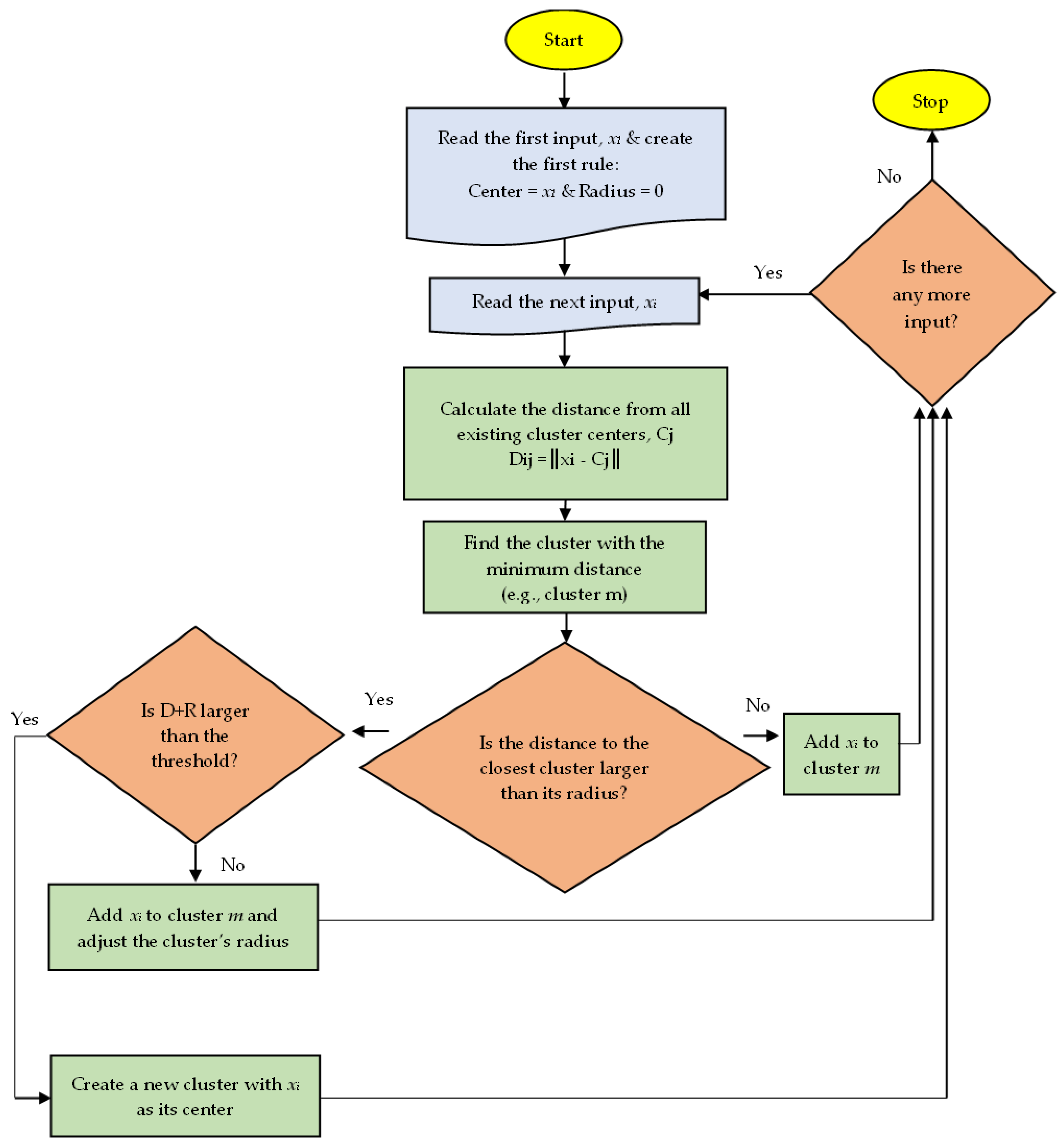
The first NFS algorithm with local learning used in hydrological modeling was the dynamic evolving neural-fuzzy inference system (DENFIS), which was originally introduced by Kasabov and Song [97]. A DENFIS employs the evolving clustering method (ECM), which is a fast, one-pass clustering algorithm that creates partitions of the input space in an incremental approach using a flow of incoming data. Figure 6 illustrates the flowchart of the ECM algorithm. One of the early applications of a DENFIS in hydrological modeling was a study by Hong and White [95] for flow forecasting in Waikoropupu Springs, New Zealand. The authors compared the results of a DENFIS with the ones obtained by an ANFIS and the back-propagation neural network, where the superiority of the DENFIS over the other two models was reported. Talei, Chua [101] employed a DENFIS for rainfall–runoff modeling in small catchments in Singapore and a large one in Sweden. The authors compared the DENFIS with an ANFIS and a few physically based models and showed DENFIS capabilities, especially in peak estimation. Heddam [102] found a DENFIS to be a promising tool for modeling dissolved oxygen in a river located in the USA. In another study, Heddam and Dechemi [103] employed a DENFIS to model the coagulant dosage in Algeria’s water treatment plant. The authors found the DENFIS to be a robust modeling tool in their study and found the local learning mechanism of the model helpful in performance accuracy. Chang, Talei [104] developed an event-based rainfall–runoff model in the Sungai Kayu Ara catchment, Malaysia, using a DENFIS and compared it with a hydrologic engineering center–hydrologic modeling system (HEC-HMS). The authors showed that the DENFIS outperformed the HEC-HMS in overall hydrograph simulation and peak estimation. Eray, Mert [105] compared a DENFIS with multi-gene genetic programming (MGGP) and genetic programming (GP) techniques in modeling pan evaporation in Antakya and Antalya stations located in Turkey. The authors found the DENFIS to be superior to other models in Antalya, while GP became the best model in Antakya. Esmaeilbeiki, Nikpour [106] compared DENFIS with multiple machine learning techniques for groundwater quality modeling. The authors found the DENFIS and gene expression programming (GEP) to be the most successful techniques when compared to others. Recently, Ye, Zahra [107] employed two metaheuristic optimization algorithms, the whale optimization algorithm (WOA) and bat algorithm (BA), to optimize the DENFIS model’s parameters for predicting evapotranspiration in the coastal region of southwest Bangladesh. The results showed that the DENFIS-WOA model outperforms other models used in this study.
Despite the successful application of a DENFIS in various hydrological modeling problems, some issues are also attached to this model. For example, the incremental learning mechanism in a DENFIS can make it sensitive to the incoming data sequence. Chang, Talei [108] studied the impact of a training data sequence on DENFIS model performance during the testing stage for a rainfall–runoff application. This study showed that the data sequence impacts the number of rules the model generates during the training stage. Moreover, it was also concluded that training the model with a sequence of low and high (or high and low) flows followed by medium flows might result in a better performance during the testing stage. The authors highlighted that a sequence of contrasting flows (i.e., low versus high) could generate more distinct rules in the system, eventually contributing to a better prediction at the testing stage. The incremental learning mechanism of a DENFIS also makes its rule base ever-expanding, as any new data tuple may result in a new cluster in the input space, which will be translated as new rules in the system [101]. As a result, the model rule base may become so large in the long run that it causes unnecessary model complexity. In addition, this incremental approach may accumulate inconsistent rules in the system as some newly generated rules may be inconsistent with the older ones. In the NFS context, inconsistent rules are the ones that have different rule consequents for similar rule antecedents. Therefore, a need for a rule-pruning mechanism arises to control the rule base size and maintain consistency in the rule base while keeping it up-to-date.
To address the incremental learning issues in NFS models such as a DENFIS, Chang, Talei [109] adopted the self-adaptive fuzzy inference network (SaFIN) for rainfall–runoff modeling applications in three distinct catchments located in China, Sweden, and Australia. The learning mechanism in a SaFIN is a self-organizing neural fuzzy system capable of local learning [100]. The clustering technique in a SaFIN is categorical learning-induced partitioning (CLIP), which updates the model for incoming data. A SaFIN has a self-automated rule generation system that runs through the partitioned data by CLIP at two stages. The first stage is the rule generation using the created clusters by CLIP. Then, in the second stage, a rule-pruning mechanism gets activated to check the rules for consistency. Once an inconsistency is identified, the rule-pruning algorithm removes the more obsolete rule. To date, a SaFIN has been compared with a DENFIS for rainfall–runoff modeling in five catchments with different sizes and types. Table 1 summarizes the performance of a SaFIN and DENFIS in these catchments in terms of the Nash–Sutcliffe coefficient of efficiency (CE), R2, RMSE, and MAE. As can be seen, the SaFIN consistently outperformed the DENFIS in all catchments in terms of different performance criteria.
Despite using local learning, the discussed studies on the DENFIS and SaFIN are still considered offline as their learning stops at the end of training stage; this means the rule base does not change anymore when the training is concluded. However, as mentioned earlier in this section, local learning is suitable for online hydrological models for real-time modeling and forecasting. For example, Talei, Chua [101] developed a real-time DENFIS model (RT-DENFIS) and examined its performance for rainfall–runoff modeling in a catchment with 43 years of daily data. The model performance was compared with an ANFIS model. The authors concluded that the ANFIS needs a yearly re-calibration to compete with the RT-DENFIS. Yu, Tan [111] used an online DENFIS to develop an ensemble modeling tool for real-time water level forecasting. Ashrafi, Chua [112] adopted the generic self-evolving Takagi–Sugeno–Kang (GSETSK) algorithm for runoff forecasting in two catchments in Vietnam and Sweden. They compared the results with the ones obtained by a DENFIS and concluded that the online GSETSK outperforms the online DENFIS. The rule-pruning mechanism in GSETSK resulted in a more compact rule base compared to the DENFIS. Similar findings were reported in another study by Ashrafi, Chua [113] where GSETSK was used for rainfall–runoff modeling and river routing applications. The reviewed studies in this section showed the promising capacities of NFS models with local learning for developing adaptive tools that can continuously learn. Such models were successfully used as real-time hydrological modeling and forecasting techniques without a need for re-calibration as their learning process never stops.

3.5. Interpretability of the NFS Models

NFS models are relatively advantageous over ANNs and other AI-based techniques because of their interpretability which, of course, is not the same in different NFS algorithms. Interpretability is because the learned knowledge from the data is structured as fuzzy rules in the rule base, from which the physics of the problem can be interpretable to some extent. Therefore, NFS algorithms are also known as grey-box models since the learned knowledge is not as hidden as in black-box models such as ANNs. However, this advantage of NFS models has not been well appreciated as the model performance in proving numerical solutions has often been the primary focus.
One of the early attempts at extracting the physics of the problem from the fuzzy rules was by Deka and Chandramouli [114] for a hydrologic flow routing application. The authors extracted linguistic rules from a fuzzy neural network (FNN) and found them helpful in decision-making processes related to flow. This study considered five fuzzy labels for flow, including very low, low, medium, high, and very high. The linguistic rules were able to explain the relationships between flow at different gauges along the river in the study site. An example of a linguistic rule extracted is presented in Equation (6):
IF flow is low at gauges I/II, THEN flow is low OR medium at gauge III
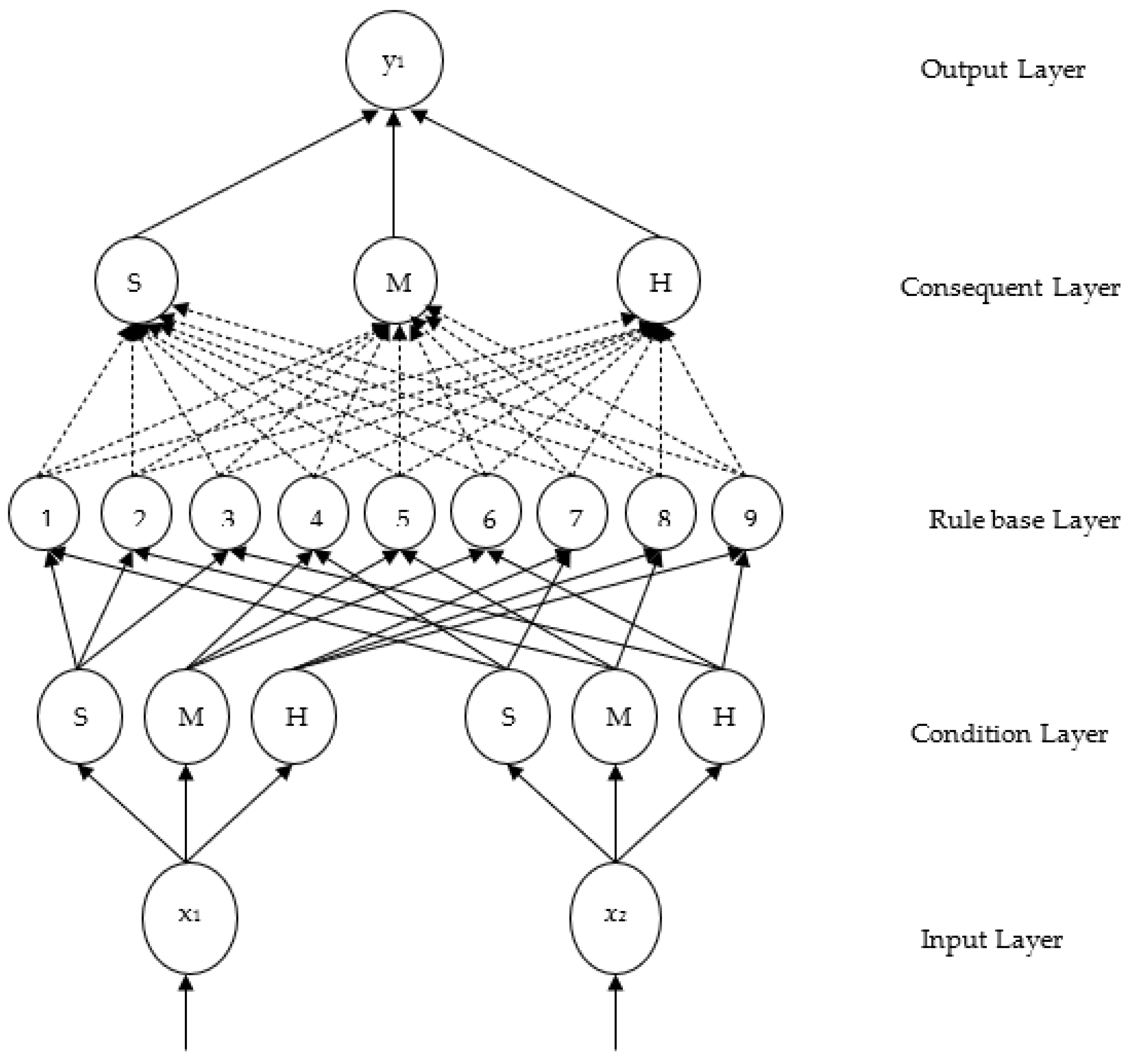
An ANFIS was also used to develop a multi-purpose reservoir’s operation policy [115]. In this study, fuzzy Mamdani (FM) and ANFIS models with grid partitioning (GP) and subtracting clustering (SC) were developed to determine the reservoir outflow (releases). The authors found the ANFIS-SC as the best model; however, FM was more user-friendly because of having flexibility in the number and type of membership functions. In addition, the authors found the extracted fuzzy IF–THEN rules useful for developing reservoir operating policies. In a flood forecasting study using a Takagi–Sugeno NFS, Nayak [116] explained the internal process of the fuzzy rule base in predicting floods for different forecast horizons. The author also identified the most dominant input variable in predicting the flow. Talei [117] compared the interpretability of Mamdani and Takagi–Sugeno NFS in a rainfall–runoff modeling application. The author showed that the rules’ fuzzy antecedent and consequent in the Mamdani FIS could be more interpretable than the Takagi–Sugeno FIS with linear functions as the rule consequent. This study adopted the pseudo outer product fuzzy neural network (POP-FNN) (Quek and Zhou, 1999) algorithm to develop rainfall–runoff models in different sizes and types of catchments. The POP-FNN consists of a five-layer network where the number of rules depends on the number of inputs and a selected number of fuzzy labels. Figure 7 illustrates the structure of a POP-FNN model for a two-input system where three fuzzy labels of low, medium, and high are considered. As can be seen, the total number of rules can be obtained by 32 = 9, where 3 is the number of labels, and 2 is the number of inputs. The results of this study showed that the POP-FNN has comparable, if not superior, results to the ANFIS in three studied catchments (located in Singapore and China). The interpretability of the rules extracted from the POP-FNN and ANFIS are compared in Table 2 for rainfall–runoff modeling in a small catchment with one rainfall and one flow gauge at the outlet [117]. In this example, the two inputs are two rainfall antecedents, while the output is the flow at the catchment outlet. For the sake of simplicity in comparison, two fuzzy labels of low (L) and high (H) are considered, resulting in 22 = 4 rules. As can be seen, the extracted rules from the POP-FNN are linguistic fuzzy IF–THEN rules where clear associations between inputs and output are demonstrated. In contrast, the rules extracted from the ANFIS have linear functions at the rule’s consequent, where the flow magnitude cannot be directly inferred. The advantage of a POP-FNN over an ANFIS in terms of interpretability is evident in this example.
In a similar attempt, Heddam [118] extracted the rules from an ANFIS model developed for water quality modeling in the Klamath river in the USA. The author extracted the linear functions between the desired output, dissolved oxygen, and inputs, including pH, specific conductance (μS/cm), and sensor depth (m). However, it was hard to interpret the associations between inputs and output from the 15 extracted rules due to the crisp outputs of the ANFIS. Chang and Tsai [119] also developed an ANFIS model coupled with a two-staged gamma test for optimal input selection in a flood forecasting application. The two fuzzy “IF–THEN” rules effectively segregate the inputs into high and low conditions, allowing the accurate prediction of different input–output scenarios. The authors highlighted that it is possible to extract valuable knowledge on the rainfall–runoff relationship by evaluating the membership functions.
Reviewing the published works on the interpretability of NFS, it is crystal clear that the Mamdani NFS is more advantageous than the Takagi–Sugeno NFS. The fuzzy IF–THEN rules that can be extracted could be helpful in applications that seek operational policies (e.g., in reservoirs, treatment plants, etc.). Further, in catchments with multiple gauging stations, such fuzzy rules could help identify dominant stations for hydrological forecasting applications such as flood prediction. However, minimal studies have been conducted on this topic, and further exploration of the interpretability of different NFS algorithms is required.

3.6. Optimization of Model Parameters

Each NFS model has its learning mechanism to find model parameters by going through the training dataset. For example, an ANFIS has two standard learning options known as grid partitioning (GP) and subtractive clustering (SC), where the latter has been found favorable relative to the former [115,120,121,122]. In general, the learning algorithm in conventional NFS models, such as an ANFIS, may get trapped in local optimum points and voluminous computations, resulting in poor accuracy [123]. Therefore, some research studies have focused on integrating NFS models with an optimizer to access more optimum model parameters, resulting in better performance. For example, Khosravi, Panahi [90] combined an ANFIS with five metaheuristic algorithms, namely invasive weed optimization (IWO), differential evolution (DE), the firefly algorithm (FA), particle swarm optimization (PSO), and the bees algorithm (BA) for spatial groundwater prediction. The authors found the ANFIS-DE to be the best model compared to other models in this study.
In a similar attempt by Azad, Karami [124] for modeling electrical conductivity, sodium absorption rate, and total hardness, ANFIS-DE was once again selected as the best model compared to integrated ANFIS models with genetic algorithm (GA) and ant colony optimization for continuous domains (ACOR). In a comparative analysis by Kisi and Yaseen [123], ANFIS models integrated with a continuous genetic algorithm (CGA), PSO, ACOR, and DE were compared in groundwater quality modeling. The authors found ANFIS-CGA to be the best-performing model compared to others. In another two studies, PSO demonstrated excellent performance in modeling the river quality [125] and groundwater table [126]. Moreover, grey wolf optimization (GWO) also showed successful integration with an ANFIS in modeling soil moisture content and demonstrated better results than those obtained by conventional ANFIS, ANN, and SVM models [127].
As can be seen, several optimization methods have been successfully integrated with conventional NFS, such as an ANFIS, to find the optimum set of model parameters resulting in better model performance. However, such improvements have been relatively modest. Furthermore, it is hard to recommend any specific optimization method as (1) multiple optimization methods have been reported as the best in different applications, and (2) their results are not significantly different. Therefore, it seems reasonable to attempt any optimizers to enhance NFS model parameters.

4. Future Directions

In Section 2, different NFS algorithms were discussed, while in Section 3, challenges in developing NFS-based hydrological models were reviewed. This section is focused on concluding notes on the past and present advancements in this field while discussing potential future research directions.
First, with recent advancements in computer science, more complex and powerful NFS algorithms are expected to be available. Therefore, employing such tools to address hydrological problems would be necessary. For example, one of the common challenges in data-driven algorithms, including NFS, is their limitation in extrapolating beyond the learning knowledge from the training dataset. Addressing such issues and enhancing the model’s performance in extreme event prediction could become possible soon using new NFS algorithms. Therefore, targeting tools based on specific needs in hydrological modeling and forecasting is necessary.
In data pre-processing, the data standardization techniques are well practiced. However, new advancements in enhancing NFS model performance using wavelet transform algorithms look promising. However, it is not clear what algorithm is the most suitable for each NFS model. Furthermore, most of the efforts in this area have focused on the ANFIS model, while other NFS models are not explored. Therefore, further studies on integrating such pre-processing methods in various NFS models look necessary.
Regarding input selection, several methods have been investigated for data-driven models, including NFS. However, no specific method has been universally recognized as the best input selection technique. That gives the users flexibility to explore the existing methods for their problem while seeking new approaches. Perhaps one interesting area to further explore is relating the selected inputs to the physics of the problem. For example, many studies have shown that using rainfall inputs from all stations in catchments with multiple rainfall stations is not necessarily the best input combination for a rainfall–runoff model. Instead, a set of selected stations would work more efficiently and accurately. In such a case, the question remains why those stations are selected. Understanding such a process and the selection mechanism used in input selection techniques could help researchers make more robust choices.
Selecting the training dataset is perhaps a less studied topic in developing NFS models. Besides the common challenge of choosing a proper dataset to train and validate the model, the sensitivity of different NFS models to the training dataset’s size, diversity, and sequence is relatively unexplored. For example, an ANFIS may not be sensitive to the sequence of data points in the training dataset. At the same time, different data sequences could affect DENFIS performance and the number of generated rules. Moreover, there is no clear guideline for the minimum required length of the training dataset. Therefore, conducting such studies on a wide range of NFS algorithms could be helpful.
On the other hand, the adaptability of NFS algorithms is an important feature that makes them helpful in developing real-time and/or adaptive forecasting tools. However, adaptability looks dependent on the learning mechanism in NFS models. In general, an online model looks necessary to adapt to environmental changes. However, such NFS online models are deemed to work effectively with local learning techniques, which are unavailable in all NFS models. Moreover, some existing models with local learning suffer from issues such as rule inconsistency, large rule base, etc. Despite addressing some of these issues by introducing a rule-pruning mechanism (e.g., in SaFIN and GSETSK), there is still a lot to explore on NFS online models for real-time modeling and forecasting.
The present literature review highlighted the importance of interpretability in NFS hydrological models, especially when operation policies are needed (e.g., reservoir operation). Therefore, it was inferred that Mamdani-type NFS models would be preferred over Takagi–Sugeno NFS due to having fuzzy antecedents and consequents in their IF–THEN rules. Despite its importance, very few studies have been focused on interpretability, and limited algorithms with such capabilities have been explored. Extracting fuzzy rules can showcase some aspects of the physics of the problem, which could be helpful in further enhancement of model performance at input variables and the training data selection stages. Therefore, in-depth studies on Mamdani-type NFS algorithms and their interpretability are needed.
Finally, by advancements in developing new optimization tools, the NFS model parameters can be found accurately to enhance model robustness in predicting the desired output. However, most studies have focused on optimizing ANFIS model parameters, while other NFS algorithms are left either unexplored or not deeply studied. Therefore, further studies on integrating optimization techniques into various NFS models are necessary.

5. Conclusions

This study reviewed the existing NFS models used in hydrological modeling and forecasting. Moreover, it discussed six common challenges in developing such models: pre-processing, input selection, training data selection, adaptability, interpretability, and parameter optimization. It was concluded that NFS algorithms have good potential for being used as a modeling and forecasting tool in various hydrological problems, including rainfall–runoff simulation, flow prediction, rainfall forecasting, water quality modeling, groundwater modeling, etc. These models generally outperform their competitors, such as regression-based models, ANNs, SVM, etc. Despite successful applications, many aspects of model development are still not fully addressed. Therefore, further studies are needed to enhance the NFS model’s performance, stability, adaptability, and interpretability. The specific conclusions of this study are six-fold:
(i)
Data pre-processing is necessary for NFS model development. All conventional methods based on data standardization would work well. Additionally, new advancements in wavelet transform functions and their successful integration into NFS algorithms suggest further study.
(ii)
Different input selection methods reported in the literature perform well in developing NFS models. However, further study is needed for cases with multiple sources of inputs (e.g., catchments with multiple rain gauges), as using more inputs may not necessarily enhance model performance.
(iii)
The sensitivity of NFS models to training datasets is yet to be explored in detail. The impact of training data size, sequence, etc., on model performance in several NFS algorithms is not explored.
(iv)
NFS models with local learning have the potential to develop online models which can be employed for adapting to hydrological changes and real-time modeling. Despite using a few algorithms, such as a DENFIS, SaFIN, and GSETSK, in hydrological modeling and forecasting, limited works have been published in this area.
(v)
The interpretability of NFS models is yet to be explored in hydrological modeling. For this, the Mamdani-type NFS with fuzzy rule consequent is advantageous over the Takagi–Sugeno NFS. The extracted linguistic IF–THEN rules could reveal the problem’s physics while helping to formulate the association between inputs and output in a qualitative manner. Further study is necessary to explore interpretability in NFS-based hydrological models
(vi)
Efforts to integrate optimization techniques into NFS models have improved the model’s performance. These studies have been mainly focused on ANFISs; however, such improvements have not been significant over the conventional NFS. Anyway, no substantial superiority has been reported in any optimization tool, meaning that using any of them could be reasonably helpful. However, further study on using optimization tools in various NFS algorithms is needed.

Author Contributions

Conceptualization, Y.K.A. and A.T.; methodology, A.T. and A.R.; software, Y.K.A. and A.T.; validation, A.T. and I.Z.; formal analysis, Y.K.A.; investigation, Y.K.A. and A.T.; resources, A.T.; data curation, Y.K.A.; writing—original draft preparation, Y.K.A. and A.T.; writing—review and editing, A.T., A.R. and I.Z.; visualization, Y.K.A.; supervision, A.T.; project administration, A.T. All authors have read and agreed to the published version of the manuscript.

Funding

This research received no external funding.

Data Availability Statement

No new data were created or analyzed in this study. Data sharing is not applicable to this article.

Conflicts of Interest

The authors declare no conflict of interest.

References

  1. Daneshmand, H.; Alaghmand, S.; Camporese, M.; Talei, A.; Daly, E. Water and salt balance modelling of intermittent catchments using a physically-based integrated model. J. Hydrol. 2018, 568, 1017–1030. [Google Scholar] [CrossRef]
  2. Singh, V.P. Hydrologic Systems. Rainfall-Runoff Modeling, Volume I; Prentice Hall: Englewood Cliffs, NJ, USA, 1988; Volume 1, p. 988. [Google Scholar]
  3. Halff, A.H.; Halff, H.; Azmoodeh, M. Predicting runoff from rainfall using neural networks. In Proceeding Engineering Hydrology; ASCE: New York, NY, USA, 1993; pp. 760–765. [Google Scholar]
  4. Nayak, P.C.; Sudheer, K.P.; Rangan, D.M.; Ramasastri, K.S. A neuro-fuzzy computing technique for modeling hydrological time series. J. Hydrol. 2004, 291, 52–66. [Google Scholar] [CrossRef]
  5. Haykin, S. Neural Networks: A Comprehensive Foundation; Prentice Hall: Englewood Cliffs, NJ, USA, 1999. [Google Scholar]
  6. Govindaraju, R.S. Artificial neural networks in hydrology. II: Hydrologic applications. J. Hydrol. Eng. 2000, 5, 124–137. [Google Scholar]
  7. Dawson, C.W.; Wilby, R.L. Hydrological modelling using artificial neural networks. Prog. Phys. Geogr. 2001, 25, 80–108. [Google Scholar] [CrossRef]
  8. Govindaraju, R.S. Artificial neural networks in hydrology. I: Preliminary concepts. J. Hydrol. Eng. 2000, 5, 115–123. [Google Scholar]
  9. Mamdani, E.H.; Assilian, S. An experiment in linguistic synthesis with a fuzzy logic controller. Int. J. Man-Mach. Stud. 1975, 7, 1–13. [Google Scholar] [CrossRef]
  10. Takagi, T.; Sugeno, M. Fuzzy Identification of Systems and Its Applications to Modeling and Control. IEEE Trans. Syst. Man Cybern. 1985, 15, 116–132. [Google Scholar] [CrossRef]
  11. Gautam, D.K.; Holz, K.P. Rainfall-runoff modelling using adaptive neuro-fuzzy systems. J. Hydroinform. 2001, 3, 3–10. [Google Scholar] [CrossRef] [Green Version]
  12. Gautam, D.K.; Holz, K.P.; Meyer, Z. Real-time forecasting of water levels using adaptive neuro-fuzzy systems. Arch. Hydroeng. Environ. Mech. 2001, 48, 3–21. [Google Scholar]
  13. Bartoletti, N.; Casagli, F.; Marsili-Libelli, S.; Nardi, A.; Palandri, L. Data-driven rainfall/runoff modelling based on a neuro-fuzzy inference system. Environ. Model. Softw. 2018, 106, 35–47. [Google Scholar] [CrossRef]
  14. Chen, S.-H.; Lin, Y.-H.; Chang, L.-C.; Chang, F.-J. The strategy of building a flood forecast model by neuro-fuzzy network. Hydrol. Process. 2005, 20, 1525–1540. [Google Scholar] [CrossRef]
  15. Kisi, O.; Shiri, J.; Tombul, M. Modeling rainfall-runoff process using soft computing techniques. Comput. Geosci. 2013, 51, 108–117. [Google Scholar] [CrossRef]
  16. Jeong, C.; Shin, J.-Y.; Kim, T.; Heo, J.-H. Monthly Precipitation Forecasting with a Neuro-Fuzzy Model. Water Resour. Manag. 2012, 26, 4467–4483. [Google Scholar] [CrossRef]
  17. Mekanik, F.; Alam Imteaz, M.; Talei, A. Seasonal rainfall forecasting by adaptive network-based fuzzy inference system (ANFIS) using large scale climate signals. Clim. Dyn. 2015, 46, 3097–3111. [Google Scholar] [CrossRef]
  18. Zeynoddin, M.; Bonakdari, H.; Azari, A.; Ebtehaj, I.; Gharabaghi, B.; Madavar, H.R. Novel hybrid linear stochastic with non-linear extreme learning machine methods for forecasting monthly rainfall a tropical climate. J. Environ. Manag. 2018, 222, 190–206. [Google Scholar] [CrossRef]
  19. Adnan, R.M.; Liang, Z.; Trajkovic, S.; Zounemat-Kermani, M.; Li, B.; Kisi, O. Daily streamflow prediction using optimally pruned extreme learning machine. J. Hydrol. 2019, 577, 123981. [Google Scholar] [CrossRef]
  20. Nayak, P.C.; Sudheer, K.P.; Rangan, D.M.; Ramasastri, K.S. Short-term flood forecasting with a neurofuzzy model. Water Resour. Res. 2005, 41, 1–16. [Google Scholar] [CrossRef] [Green Version]
  21. Sanikhani, H.; Kisi, O. River Flow Estimation and Forecasting by Using Two Different Adaptive Neuro-Fuzzy Approaches. Water Resour. Manag. 2012, 26, 1715–1729. [Google Scholar] [CrossRef]
  22. Shiri, J.; Kisi, O. Short-term and long-term streamflow forecasting using a wavelet and neuro-fuzzy conjunction model. J. Hydrol. 2010, 394, 486–493. [Google Scholar] [CrossRef]
  23. Dixon, B. Applicability of neuro-fuzzy techniques in predicting ground-water vulnerability: A GIS-based sensitivity analysis. J. Hydrol. 2005, 309, 17–38. [Google Scholar] [CrossRef]
  24. Kholghi, M.; Hosseini, S.M. Comparison of Groundwater Level Estimation Using Neuro-fuzzy and Ordinary Kriging. Environ. Model. Assess. 2009, 14, 729–737. [Google Scholar] [CrossRef]
  25. Shirmohammadi, B.; Vafakhah, M.; Moosavi, V.; Moghaddamnia, A. Application of Several Data-Driven Techniques for Predicting Groundwater Level. Water Resour. Manag. 2013, 27, 419–432. [Google Scholar] [CrossRef]
  26. Ikram, R.M.A.; Jaafari, A.; Milan, S.G.; Kisi, O.; Heddam, S.; Zounemat-Kermani, M. Hybridized Adaptive Neuro-Fuzzy Inference System with Metaheuristic Algorithms for Modeling Monthly Pan Evaporation. Water 2022, 14, 3549. [Google Scholar] [CrossRef]
  27. Goyal, M.K.; Bharti, B.; Quilty, J.; Adamowski, J.; Pandey, A. Modeling of daily pan evaporation in sub tropical climates using ANN, LS-SVR, Fuzzy Logic, and ANFIS. Expert Syst. Appl. 2014, 41, 5267–5276. [Google Scholar] [CrossRef]
  28. Kişi, Ö.; Öztürk, Ö. Adaptive Neurofuzzy Computing Technique for Evapotranspiration Estimation. J. Irrig. Drain. Eng. 2007, 133, 368–379. [Google Scholar] [CrossRef]
  29. Wang, L.; Kisi, O.; Hu, B.; Bilal, M.; Zounemat-Kermani, M.; Li, H. Evaporation modelling using different machine learning techniques. Int. J. Clim. 2017, 37, 1076–1092. [Google Scholar] [CrossRef]
  30. Ly, Q.V.; Nguyen, X.C.; Lê, N.C.; Truong, T.-D.; Hoang, T.-H.T.; Park, T.J.; Maqbool, T.; Pyo, J.; Cho, K.H.; Lee, K.-S.; et al. Application of Machine Learning for eutrophication analysis and algal bloom prediction in an urban river: A 10-year study of the Han River, South Korea. Sci. Total Environ. 2021, 797, 149040. [Google Scholar] [CrossRef]
  31. Parmar, K.S.; Makkhan, S.J.S.; Kaushal, S. Neuro-fuzzy-wavelet hybrid approach to estimate the future trends of river water quality. Neural Comput. Appl. 2019, 31, 8463–8473. [Google Scholar] [CrossRef]
  32. Yeon, I.S.; Kim, J.H.; Jun, K.W. Application of artificial intelligence models in water quality forecasting. Environ. Technol. 2008, 29, 625–631. [Google Scholar] [CrossRef]
  33. Ghavidel, S.Z.Z.; Montaseri, M. Application of different data-driven methods for the prediction of total dissolved solids in the Zarinehroud basin. Stoch. Environ. Res. Risk Assess. 2014, 28, 2101–2118. [Google Scholar] [CrossRef]
  34. Idrees, M.B.; Jehanzaib, M.; Kim, D.; Kim, T.-W. Comprehensive evaluation of machine learning models for suspended sediment load inflow prediction in a reservoir. Stoch. Environ. Res. Risk Assess. 2021, 35, 1805–1823. [Google Scholar] [CrossRef]
  35. Kisi, O.; Zounemat-Kermani, M. Suspended Sediment Modeling Using Neuro-Fuzzy Embedded Fuzzy c-Means Clustering Technique. Water Resour. Manag. 2016, 30, 3979–3994. [Google Scholar] [CrossRef]
  36. Rajaee, T.; Mirbagheri, S.A.; Zounemat-Kermani, M.; Nourani, V. Daily suspended sediment concentration simulation using ANN and neuro-fuzzy models. Sci. Total Environ. 2009, 407, 4916–4927. [Google Scholar] [CrossRef]
  37. Jang, J.-S.R. ANFIS: Adaptive-Network-Based Fuzzy Inference System. IEEE Trans. Syst. Man Cybern. 1993, 23, 665–685. [Google Scholar] [CrossRef]
  38. Karray, F.O.; De Silva, C.W. Soft Computing and Intelligent Systems Design: Theory, Tools and Applications; Addison Wesley Longman: White Plains, NY, USA, 2004. [Google Scholar]
  39. Lin, C.-T.; Lee, C. Neural-network-based fuzzy logic control and decision system. IEEE Trans. Comput. 1991, 40, 1320–1336. [Google Scholar] [CrossRef]
  40. Nauck, D.; Klawonn, F.; Kruse, R. Foundations of Neuro-Fuzzy Systems; John Wiley & Sons, Inc.: New York, NY, USA, 1997. [Google Scholar]
  41. Talei, A.; Chua, L.H.C.; Wong, T.S. Evaluation of rainfall and discharge inputs used by Adaptive Network-based Fuzzy Inference Systems (ANFIS) in rainfall–runoff modeling. J. Hydrol. 2010, 391, 248–262. [Google Scholar] [CrossRef]
  42. Beker, H.; Piper, F. The principles of cryptography, part IV: Stream ciphers, section a: Randomness. Secur. Speech Comm. Acad. Press Chapter 1985, 3, 104–109. [Google Scholar]
  43. Akrami, S.A.; El-Shafie, A.; Jaafar, O. Improving Rainfall Forecasting Efficiency Using Modified Adaptive Neuro-Fuzzy Inference System (MANFIS). Water Resour. Manag. 2013, 27, 3507–3523. [Google Scholar] [CrossRef]
  44. Heddam, S.; Bermad, A.; Dechemi, N. ANFIS-based modelling for coagulant dosage in drinking water treatment plant: A case study. Environ. Monit. Assess. 2012, 184, 1953–1971. [Google Scholar] [CrossRef]
  45. Emamgholizadeh, S.; Moslemi, K.; Karami, G. Prediction the Groundwater Level of Bastam Plain (Iran) by Artificial Neural Network (ANN) and Adaptive Neuro-Fuzzy Inference System (ANFIS). Water Resour. Manag. 2014, 28, 5433–5446. [Google Scholar] [CrossRef]
  46. Abba, S.; Abdulkadir, R.A.; Gaya, M.; Saleh, M.; Esmaili, P.; Jibril, M.B. Neuro-fuzzy ensemble techniques for the prediction of turbidity in water treatment plant. In Proceedings of the 2019 2nd International Conference of the IEEE Nigeria Computer Chapter, NigeriaComputConf, Zaria, Nigeria, 14–17 October 2019. [Google Scholar]
  47. Khaki, M.; Yusoff, I.; Islami, N. Simulation of groundwater level through artificial intelligence system. Environ. Earth Sci. 2015, 73, 8357–8367. [Google Scholar] [CrossRef]
  48. Sönmez, A.Y.; Kale, S.; Ozdemir, R.C.; Kadak, A.E. An adaptive neuro-fuzzy inference system (ANFIS) to predict of cadmium (Cd) concentrations in the filyos river, Turkey. Turk. J. Fish. Aquat. Sci. 2018, 18, 1333–1343. [Google Scholar] [CrossRef]
  49. Van Ooyen, A.; Nienhuis, B. Improving the convergence of the back-propagation algorithm. Neural Netw. 1992, 5, 465–471. [Google Scholar] [CrossRef]
  50. Aqil, M.; Kita, I.; Yano, A.; Nishiyama, S. Analysis and prediction of flow from local source in a river basin using a Neuro-fuzzy modeling tool. J. Environ. Manag. 2007, 85, 215–223. [Google Scholar] [CrossRef]
  51. Moosavi, V.; Vafakhah, M.; Shirmohammadi, B.; Behnia, N. A Wavelet-ANFIS Hybrid Model for Groundwater Level Forecasting for Different Prediction Periods. Water Resour. Manag. 2013, 27, 1301–1321. [Google Scholar] [CrossRef]
  52. Barzegar, R.; Adamowski, J.; Moghaddam, A.A. Application of wavelet-artificial intelligence hybrid models for water quality prediction: A case study in Aji-Chay River, Iran. Stoch. Environ. Res. Risk Assess. 2016, 30, 1797–1819. [Google Scholar] [CrossRef]
  53. Fu, Z.; Cheng, J.; Yang, M.; Batista, J. Prediction of industrial wastewater quality parameters based on wavelet de-noised ANFIS model. In Proceedings of the 2018 IEEE 8th Annual Computing and Communication Workshop and Conference, CCWC, Las Vegas, NV, USA, 8–10 January 2018. [Google Scholar]
  54. Poul, A.K.; Shourian, M.; Ebrahimi, H. A Comparative Study of MLR, KNN, ANN and ANFIS Models with Wavelet Transform in Monthly Stream Flow Prediction. Water Resour. Manag. 2019, 33, 2907–2923. [Google Scholar] [CrossRef]
  55. Ahmed, A.N.; Othman, F.B.; Afan, H.A.; Ibrahim, R.K.; Fai, C.M.; Hossain, S.; Ehteram, M.; Elshafie, A. Machine learning methods for better water quality prediction. J. Hydrol. 2019, 578, 124084. [Google Scholar] [CrossRef]
  56. Shabri, A. A hybrid wavelet analysis and adaptive neuro-fuzzy inference system for drought forecasting. Appl. Mathe-Matical Sci. 2014, 8, 6909–6918. [Google Scholar] [CrossRef]
  57. Kisi, O.; Shiri, J. Wavelet and neuro-fuzzy conjunction model for predicting water table depth fluctuations. Hydrol. Res. 2012, 43, 286–300. [Google Scholar] [CrossRef]
  58. Sehgal, V.; Sahay, R.R.; Chatterjee, C. Effect of Utilization of Discrete Wavelet Components on Flood Forecasting Per-formance of Wavelet Based ANFIS Models. Water Resour. Manag. 2014, 28, 1733–1749. [Google Scholar] [CrossRef]
  59. Seo, Y.; Kim, S.; Kisi, O.; Singh, V.P. Daily water level forecasting using wavelet decomposition and artificial intelligence techniques. J. Hydrol. 2015, 520, 224–243. [Google Scholar] [CrossRef]
  60. Nourani, V.; Alami, M.T.; Vousoughi, F.D. Hybrid of SOM-Clustering Method and Wavelet-ANFIS Approach to Model and Infill Missing Groundwater Level Data. J. Hydrol. Eng. 2016, 21, 05016018. [Google Scholar] [CrossRef]
  61. Nourani, V.; Partoviyan, A. Hybrid denoising-jittering data pre-processing approach to enhance multi-step-ahead rainfall–runoff modeling. Stoch. Environ. Res. Risk Assess. 2017, 32, 545–562. [Google Scholar] [CrossRef]
  62. Abda, Z.; Chettih, M. Forecasting daily flow rate-based intelligent hybrid models combining wavelet and Hilbert–Huang transforms in the mediterranean basin in northern Algeria. Acta Geophys. 2018, 66, 1131–1150. [Google Scholar] [CrossRef]
  63. Chang, F.-J.; Chang, Y.-T. Adaptive neuro-fuzzy inference system for prediction of water level in reservoir. Adv. Water Resour. 2006, 29, 1–10. [Google Scholar] [CrossRef]
  64. Esmaeelzadeh, S.R.; Adib, A.; Alahdin, S. Long-term streamflow forecasts by Adaptive Neuro-Fuzzy Inference System using satellite images and K-fold cross-validation (Case study: Dez, Iran). KSCE J. Civ. Eng. 2014, 19, 2298–2306. [Google Scholar] [CrossRef]
  65. Ali, M.; Deo, R.C.; Downs, N.J.; Maraseni, T. Multi-stage committee based extreme learning machine model incorporating the influence of climate parameters and seasonality on drought forecasting. Comput. Electron. Agric. 2018, 152, 149–165. [Google Scholar] [CrossRef]
  66. Lohani, A.; Kumar, R.; Singh, R. Hydrological time series modeling: A comparison between adaptive neuro-fuzzy, neural network and autoregressive techniques. J. Hydrol. 2012, 442–443, 23–35. [Google Scholar] [CrossRef]
  67. Doǧan, E. Reference evapotranspiration estimation using adaptive neuro-fuzzy inference systems. Irrig. Drain. 2009, 58, 617–628. [Google Scholar] [CrossRef]
  68. Stefánsson, A.; Končar, N.; Jones, A.J. A note on the gamma test. Neural Comput. Appl. 1997, 5, 131–133. [Google Scholar] [CrossRef]
  69. Malik, A.; Kumar, A.; Kisi, O. Monthly pan-evaporation estimation in Indian central Himalayas using different heuristic approaches and climate based models. Comput. Electron. Agric. 2017, 143, 302–313. [Google Scholar] [CrossRef]
  70. Moghaddamnia, A.; Gousheh, M.G.; Piri, J.; Amin, S.; Han, D. Evaporation estimation using artificial neural networks and adaptive neuro-fuzzy inference system techniques. Adv. Water Resour. 2009, 32, 88–97. [Google Scholar] [CrossRef]
  71. Malik, A.; Kumar, A.; Piri, J. Daily suspended sediment concentration simulation using hydrological data of Pranhita River Basin, India. Comput. Electron. Agric. 2017, 138, 20–28. [Google Scholar] [CrossRef]
  72. Dodangeh, E.; Ewees, A.A.; Shahid, S.; Yaseen, Z.M. Daily scale river flow simulation: Hybridized fuzzy logic model with metaheuristic algorithms. Hydrol. Sci. J. 2021, 66, 2155–2169. [Google Scholar] [CrossRef]
  73. Wan, J.; Huang, M.; Ma, Y.; Guo, W.; Wang, Y.; Zhang, H.; Li, W.; Sun, X. Prediction of effluent quality of a paper mill wastewater treatment using an adaptive network-based fuzzy inference system. Appl. Soft Comput. 2011, 11, 3238–3246. [Google Scholar] [CrossRef]
  74. Civelekoglu, G.; Perendeci, A.; Yigit, N.O.; Kitis, M. Modeling Carbon and Nitrogen Removal in an Industrial Wastewater Treatment Plant Using an Adaptive Network-Based Fuzzy Inference System. CLEAN—Soil Air Water 2007, 35, 617–625. [Google Scholar] [CrossRef]
  75. Civelekoglu, G.; Yigit, N.O.; Diamadopoulos, E.; Kitis, M. Modelling of COD removal in a biological wastewater treatment plant using adaptive neuro-fuzzy inference system and artificial neural network. Water Sci. Technol. 2009, 60, 1475–1487. [Google Scholar] [CrossRef]
  76. Parsaie, A.; Haghiabi, A.H. Prediction of discharge coefficient of side weir using adaptive neuro-fuzzy inference system. Sustain. Water Resour. Manag. 2016, 2, 257–264. [Google Scholar] [CrossRef] [Green Version]
  77. Aqil, M.; Kita, I.; Yano, A.; Nishiyama, S. A comparative study of artificial neural networks and neuro-fuzzy in continuous modeling of the daily and hourly behaviour of runoff. J. Hydrol. 2007, 337, 22–34. [Google Scholar] [CrossRef]
  78. Nawaz, N.; Harun, S.; Talei, A. Application of adaptive network-based fuzzy inference system (ANFIS) for river stage prediction in a tropical catchment. Appl. Mech. Mater. 2015, 735, 195–199. [Google Scholar] [CrossRef]
  79. Gong, Y.; Wang, Z.; Xu, G.; Zhang, Z. A Comparative Study of Groundwater Level Forecasting Using Data-Driven Models Based on Ensemble Empirical Mode Decomposition. Water 2018, 10, 730. [Google Scholar] [CrossRef] [Green Version]
  80. Nguyen, P.K.-T.; Chua, L.H.-C.; Talei, A.; Chai, Q.H. Water level forecasting using neuro-fuzzy models with local learning. Neural Comput. Appl. 2018, 30, 1877–1887. [Google Scholar] [CrossRef]
  81. Nguyen, P.K.-T.; Chua, L.H.-C.; Son, L.H. Flood forecasting in large rivers with data-driven models. Nat. Hazards 2014, 71, 767–784. [Google Scholar] [CrossRef]
  82. Sun, Y.; Tang, D.; Sun, Y.; Cui, Q. Comparison of a fuzzy control and the data-driven model for flood forecasting. Nat. Hazards 2016, 82, 827–844. [Google Scholar] [CrossRef]
  83. Üneş, F.; Kaya, Y.Z.; Mamak, M. Daily reference evapotranspiration prediction based on climatic conditions applying different data mining techniques and empirical equations. Theor. Appl. Clim. 2020, 141, 763–773. [Google Scholar] [CrossRef]
  84. Lee, M.Z.; Mekanik, F.; Talei, A. Dynamic Neuro-Fuzzy Systems for Forecasting El Niño Southern Oscillation (ENSO) Using Oceanic and Continental Climate Parameters as Inputs. J. Mar. Sci. Eng. 2022, 10, 1161. [Google Scholar] [CrossRef]
  85. Chang, T.K.; Talei, A.; Alaghmand, S.; Ooi, M.P.L. Choice of rainfall inputs for event-based rainfall-runoff modeling in a catchment with multiple rainfall stations using data-driven techniques. J. Hydrol. 2017, 545, 100–108. [Google Scholar] [CrossRef]
  86. Talei, A.; Chua, L.H. Influence of lag time on event-based rainfall–runoff modeling using the data driven approach. J. Hydrol. 2012, 438–439, 223–233. [Google Scholar] [CrossRef]
  87. Firat, M.; Güngör, M. Hydrological time-series modelling using an adaptive neuro-fuzzy inference system. Hydrol. Process. 2008, 22, 2122–2132. [Google Scholar] [CrossRef]
  88. Singh, S.K.; Bárdossy, A. Calibration of hydrological models on hydrologically unusual events. Adv. Water Resour. 2012, 38, 81–91. [Google Scholar] [CrossRef]
  89. Firat, M.; Güngör, M. River flow estimation using adaptive neuro fuzzy inference system. Math. Comput. Simul. 2007, 75, 87–96. [Google Scholar] [CrossRef]
  90. Khosravi, K.; Panahi, M.; Tien Bui, D. Spatial prediction of groundwater spring potential mapping based on an adaptive neuro-fuzzy inference system and metaheuristic optimization. Hydrol. Earth Syst. Sci. 2018, 22, 4771–4792. [Google Scholar] [CrossRef] [Green Version]
  91. Karimaldini, F.; Teang Shui, L.; Ahmed Mohamed, T.; Abdollahi, M.; Khalili, N. Daily evapotranspiration modeling from limited weather data by using neuro-fuzzy computing tech-nique. J. Irrig. Drain. Eng. 2012, 138, 21–34. [Google Scholar] [CrossRef] [Green Version]
  92. Shiri, J.; Keshavarzi, A.; Kisi, O.; Karimi, S. Using soil easily measured parameters for estimating soil water capacity: Soft computing approaches. Comput. Electron. Agric. 2017, 141, 327–339. [Google Scholar] [CrossRef]
  93. Talei, A.; Chua, L.H.C.; Quek, C. A novel application of a neuro-fuzzy computational technique in event-based rain-fall-runoff modeling. Expert Syst. Appl. 2010, 37, 7456–7468. [Google Scholar] [CrossRef]
  94. Zhang, S.; Lu, L.; Yu, J.; Zhou, H. Short-term water level prediction using different artificial intelligent models. In Proceedings of the 2016 5th International Conference on Agro-Geoinformatics, Agro-Geoinformatics, Tianjin, China, 18–20 July 2016; pp. 1–6. [Google Scholar]
  95. Hong, Y.-S.T.; White, P.A. Hydrological modeling using a dynamic neuro-fuzzy system with on-line and local learning algorithm. Adv. Water Resour. 2009, 32, 110–119. [Google Scholar] [CrossRef]
  96. Kasabov, N. Evolving fuzzy neural networks for supervised/unsupervised online knowledge-based learning. IEEE Trans. Syst. Man Cybern. Part B (Cybernetics) 2001, 31, 902–918. [Google Scholar] [CrossRef]
  97. Kasabov, N.K.; Song, Q. DENFIS: Dynamic evolving neural-fuzzy inference system and its application for time-series prediction. IEEE Trans. Fuzzy Syst. 2002, 10, 144–154. [Google Scholar] [CrossRef] [Green Version]
  98. Nguyen, N.N.; Zhou, W.J.; Quek, C. GSETSK: A generic self-evolving TSK fuzzy neural network with a novel Hebbi-an-based rule reduction approach. Appl. Soft Comput. J. 2015, 35, 29–42. [Google Scholar] [CrossRef]
  99. Quah, K.H.; Quek, C. FITSK: Online local learning with generic fuzzy input Takagi-Sugeno-Kang fuzzy framework for nonlinear system estimation. IEEE Trans. Syst. Man Cybern. Part B (Cybernetics) 2006, 36, 166–178. [Google Scholar] [CrossRef]
  100. Tung, S.W.; Quek, C.; Guan, C. SaFIN: A Self-Adaptive Fuzzy Inference Network. IEEE Trans. Neural Netw. 2011, 22, 1928–1940. [Google Scholar] [CrossRef]
  101. Talei, A.; Chua, L.H.C.; Quek, C.; Jansson, P.-E. Runoff forecasting using a Takagi–Sugeno neuro-fuzzy model with online learning. J. Hydrol. 2013, 488, 17–32. [Google Scholar] [CrossRef]
  102. Heddam, S. Modelling hourly dissolved oxygen concentration (DO) using dynamic evolving neural-fuzzy inference system (DENFIS)-based approach: Case study of Klamath River at Miller Island Boat Ramp, OR, USA. Environ. Sci. Pollut. Res. 2014, 21, 9212–9227. [Google Scholar] [CrossRef]
  103. Heddam, S.; Dechemi, N. A new approach based on the dynamic evolving neural-fuzzy inference system (DENFIS) for modelling coagulant dosage (Dos): Case study of water treatment plant of Algeria. Desalination Water Treat. 2015, 53, 1045–1053. [Google Scholar] [CrossRef]
  104. Kwin, C.T.; Talei, A.; Alaghmand, S.; Chua, L.H. Rainfall-runoff Modeling Using Dynamic Evolving Neural Fuzzy Inference System with Online Learning. Procedia Eng. 2016, 154, 1103–1109. [Google Scholar] [CrossRef] [Green Version]
  105. Eray, O.; Mert, C.; Kisi, O. Comparison of multi-gene genetic programming and dynamic evolving neural-fuzzy inference system in modeling pan evaporation. Hydrol. Res. 2018, 49, 1221–1233. [Google Scholar] [CrossRef]
  106. Esmaeilbeiki, F.; Nikpour, M.R.; Singh, V.K.; Kisi, O.; Sihag, P.; Sanikhani, H. Exploring the application of soft computing techniques for spatial evaluation of groundwater quality variables. J. Clean. Prod. 2020, 276, 124206. [Google Scholar] [CrossRef]
  107. Ye, L.; Zahra, M.M.A.; Al-Bedyry, N.K.; Yaseen, Z.M. Daily scale evapotranspiration prediction over the coastal region of southwest Bangladesh: New development of artificial intelligence model. Stoch. Environ. Res. Risk Assess. 2022, 36, 451–471. [Google Scholar] [CrossRef]
  108. Chang, T.K.; Talei, A.; Chua, L.H.C.; Alaghmand, S. The Impact of Training Data Sequence on the Performance of Neuro-Fuzzy Rainfall-Runoff Models with Online Learning. Water 2018, 11, 52. [Google Scholar] [CrossRef] [Green Version]
  109. Chang, T.K.; Talei, A.; Quek, C.; Pauwels, V.R. Rainfall-runoff modelling using a self-reliant fuzzy inference network with flexible structure. J. Hydrol. 2018, 564, 1179–1193. [Google Scholar] [CrossRef]
  110. Chang, T.K.; Talei, A.; Quek, C. Rainfall-runoff modelling in a semi-urbanized catchment using self-adaptive Fuzzy In-ference Network. In Proceedings of the 10th International Joint Conference on Computational Intelligence—IJCCI 2018, Seville, Spain, 18–20 September 2018. [Google Scholar]
  111. Yu, L.; Tan, S.K.; Chua, L.H.C. Online Ensemble Modeling for Real Time Water Level Forecasts. Water Resour. Manag. 2017, 31, 1105–1119. [Google Scholar] [CrossRef]
  112. Ashrafi, M.; Chua, L.H.C.; Quek, C.; Qin, X. A fully-online Neuro-Fuzzy model for flow forecasting in basins with limited data. J. Hydrol. 2017, 545, 424–435. [Google Scholar] [CrossRef]
  113. Ashrafi, M.; Chua, L.H.C.; Quek, C. The applicability of Generic Self-Evolving Takagi-Sugeno-Kang neuro-fuzzy model in modeling rainfall–runoff and river routing. Hydrol. Res. 2019, 50, 991–1001. [Google Scholar] [CrossRef]
  114. Deka, P.; Chandramouli, V. Fuzzy Neural Network Model for Hydrologic Flow Routing. J. Hydrol. Eng. 2005, 10, 302–314. [Google Scholar] [CrossRef]
  115. Mehta, R.; Jain, S.K. Optimal Operation of a Multi-Purpose Reservoir Using Neuro-Fuzzy Technique. Water Resour. Manag. 2009, 23, 509–529. [Google Scholar] [CrossRef]
  116. Nayak, P.C. Explaining Internal Behavior in a Fuzzy If-Then Rule-Based Flood-Forecasting Model. J. Hydrol. Eng. 2010, 15, 20–28. [Google Scholar] [CrossRef]
  117. Talei, A. Rainfall-Runoff Modelling with Neuro-Fuzzy Systems. Ph.D. Thesis, Nanyang Technological University, Singapore, 2013; p. 247. Available online: https://hdl.handle.net/10356/54946 (accessed on 15 November 2022).
  118. Heddam, S. Modeling hourly dissolved oxygen concentration (DO) using two different adaptive neuro-fuzzy inference systems (ANFIS): A comparative study. Environ. Monit. Assess. 2014, 186, 597–619. [Google Scholar] [CrossRef]
  119. Chang, F.-J.; Tsai, M.-J. A nonlinear spatio-temporal lumping of radar rainfall for modeling multi-step-ahead inflow forecasts by data-driven techniques. J. Hydrol. 2016, 535, 256–269. [Google Scholar] [CrossRef]
  120. Muhammad Adnan, R.; Yuan, X.; Kisi, O.; Yuan, Y.; Tayyab, M.; Lei, X. Application of soft computing models in streamflow forecasting. Proc. Inst. Civ. Eng. Water Manag. 2019, 172, 123–134. [Google Scholar] [CrossRef]
  121. Cobaner, M. Evapotranspiration estimation by two different neuro-fuzzy inference systems. J. Hydrol. 2011, 398, 292–302. [Google Scholar] [CrossRef]
  122. Montaseri, M.; Ghavidel, S.Z.Z.; Sanikhani, H. Water quality variations in different climates of Iran: Toward modeling total dissolved solid using soft computing techniques. Stoch. Environ. Res. Risk Assess. 2018, 32, 2253–2273. [Google Scholar] [CrossRef]
  123. Kisi, O.; Yaseen, Z.M. The potential of hybrid evolutionary fuzzy intelligence model for suspended sediment concentration prediction. Catena 2019, 174, 11–23. [Google Scholar] [CrossRef]
  124. Azad, A.; Karami, H.; Farzin, S.; Saeedian, A.; Kashi, H.; Sayyahi, F. Prediction of water quality parameters using ANFIS optimized by intelligence algorithms (case study: Gor-ganrood river). KSCE J. Civ. Eng. 2018, 22, 2206–2213. [Google Scholar] [CrossRef]
  125. Azad, A.; Karami, H.; Farzin, S.; Mousavi, S.-F.; Kisi, O. Modeling river water quality parameters using modified adaptive neuro fuzzy inference system. Water Sci. Eng. 2019, 12, 45–54. [Google Scholar] [CrossRef]
  126. Jahanara, A.-A.; Khodashenas, S.R. Prediction of Ground Water Table Using NF-GMDH Based Evolutionary Algorithms. KSCE J. Civ. Eng. 2019, 23, 5235–5243. [Google Scholar] [CrossRef]
  127. Maroufpoor, S.; Maroufpoor, E.; Bozorg-Haddad, O.; Shiri, J.; Yaseen, Z.M. Soil moisture simulation using hybrid artificial intelligent model: Hybridization of adaptive neuro fuzzy inference system with grey wolf optimizer algorithm. J. Hydrol. 2019, 575, 544–556. [Google Scholar] [CrossRef]
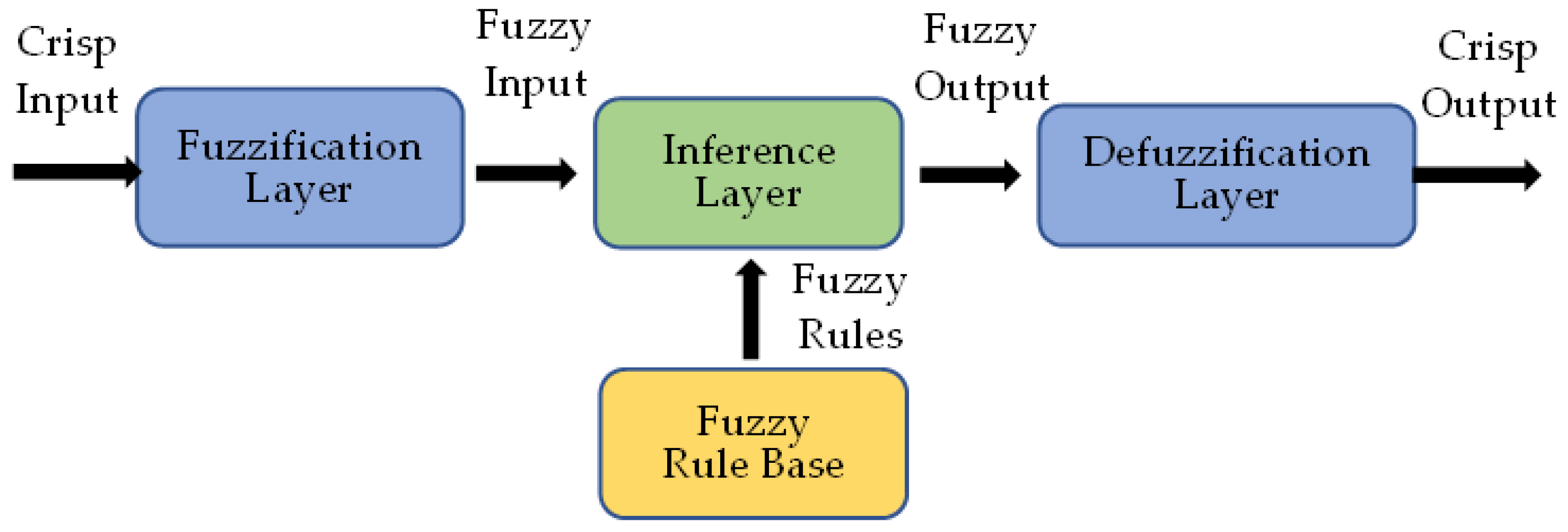
Figure 1. Schematic demonstration of a FIS.
Hydrology 10 00036 g001
Figure 2. Typical fuzzy membership functions for a variable x: a smooth curve (left) and a linear function (right).
Hydrology 10 00036 g002
Figure 3. Cooperative neuro-fuzzy systems: (a) Type 1, (b) Type 2, (c) Type 3, and (d) Type 4.
Hydrology 10 00036 g003
Figure 4. Schematic demonstration of ANFIS structure.
Hydrology 10 00036 g004
Figure 5. Schematic demonstration of a 5-fold leave-one-out cross-validation process.
Hydrology 10 00036 g005
Figure 6. Flowchart of ECM algorithm used in DENFIS model.
Hydrology 10 00036 g006
Figure 7. Schematic structure of POP-FNN for two inputs—one output scenario using three fuzzy labels of low (L), medium (M), and high (H).
Hydrology 10 00036 g007
Table 1. SaFIN and DENFIS performances for rainfall–runoff modeling in catchments with different sizes and types.
Catchment (Country)TypeArea (km2)ModelCER2MAE (m3/s)Reference
Sungai Kayu Ara (Malaysia)Urbanized23.22SaFIN0.8510.8683.021Chang, Talei [110]
DENFIS0.7960.8453.252Chang, Talei [104]
Dandenong (Australia)Semi-urbanized272SaFIN0.8930.9000.468Chang, Talei [110]
DENFIS0.8120.8430.881Unpublished-presented by the authors
Clarence (Australia)Rural with minor development22,400SaFIN0.8210.83881.608Chang, Talei [109]
DENFIS0.6700.670106.191Chang, Talei [109]
Heshui (China)Rural with minor development2275SaFIN0.8390.8496.222Chang, Talei [109]
DENFIS0.8210.8237.400Chang, Talei [109]
Klippan_2 (Sweden)Rural241.33SaFIN0.9180.9190.536Chang, Talei [109]
DENFIS0.8990.9030.601Chang, Talei [109]
Table 2. Sample extracted rules from POP-FNN and ANFIS rainfall–runoff models for two rainfall inputs and flow as output when two fuzzy labels of low (L) and high (H) are chosen.
Rule NumberInput X1Input X2Output Y (POP-FNN)Output Y (ANFIS)
1LLLY = 1.213X1 + 0.548X2 − 0.069
2LHLY = −0.297X1 + 0.172X2 + 0.043
3HLHY = 1.467X1 − 1.140X2 − 0.026
4HHHY = −5.228X1 − 0.851X2 + 5.153
Disclaimer/Publisher’s Note: The statements, opinions and data contained in all publications are solely those of the individual author(s) and contributor(s) and not of MDPI and/or the editor(s). MDPI and/or the editor(s) disclaim responsibility for any injury to people or property resulting from any ideas, methods, instructions or products referred to in the content.