Abstract
This paper proposes the development of a robust nonlinear soft sensor for online estimation of product compositions in a Heat-Integrated Distillation Column (HIDiC). Traditional composition analyzers, such as gas chromatographs, are costly and suffer from long measurement delays, making them inefficient for real-time monitoring and control. To address this, data-driven soft sensors are developed using tray temperature data obtained from a high-fidelity dynamic HIDiC simulation. The study investigates both linear and nonlinear modeling strategies for composition estimation, including principal component regression (PCR), artificial neural networks (ANNs), and, for the first time in HIDiC modeling, a Bidirectional Long Short-Term Memory (BiLSTM) network. The objective is to evaluate the capability of each method for accurate estimation of product compositions in a HIDiC. The results demonstrate that the BiLSTM-based soft sensor significantly outperforms conventional methods and offers strong potential for enhancing real-time composition estimation and control in HIDiC systems.
1. Introduction
Heat-Integrated Distillation Columns (HIDiCs) represent a cutting-edge advancement in distillation technology, designed to enhance energy efficiency through internal heat integration. Unlike conventional distillation systems, HIDiCs facilitate direct heat transfer between the rectifying and stripping sections by exploiting boiling point differences, thereby improving separation efficiency and reducing energy demand [1].
Numerous control strategies have been proposed to manage the inherent complexity and strong interactions within HIDiCs. Bisgaard et al. [2] conducted a systematic analysis to identify appropriate manipulated and controlled variables through degree-of-freedom analysis, operational mapping, and constraint identification. Their dual-layer strategy, combining regulatory and supervisory control, showed effective performance in dynamic simulations. For the control of a high-purity heat-integrated distillation column, an adaptively corrected setpoint sensitive-stage temperature control technique is suggested in [3]. First, the temperature profile movement situation, which primarily includes the functions of the temperature profile and its moving velocity, is established to characterize the dynamics of the system and ensure the logic of the setpoint correction. The temperature profile function conveys the shape of the stage’s temperature distribution, and the temperature profile’s moving velocity indicates changes in the position of the profile. The temperature measurement locations are then chosen using a modified version of the principal component analysis (PCA) approach, and the profile function’s parameters are computed using the chosen observations. In [4], diverse heat-integrated pressure swing distillation processes, such as conventional and entrainer-assisted pressure swing distillation, partially and fully heat-integrated pressure swing distillation methods all employ differential temperature control to regulate the sensitive-stage temperature under operation pressure fluctuations of the high-pressure column. Under operational pressure variations, the differential temperature control adjusts slightly, producing useful outcomes. The computation of the integral absolute error of product purities confirms that the dynamic performances of differential temperature control and pressure-compensated temperature control for each process are nearly identical.
In [5], the mixture was separated through the pervaporation process, and all reactive distillation and pervaporation-related parameters—such as permeate stream pressure, the number of modules, and the temperature of the inflow to each module—were considered optimization variables. All variables were simultaneously optimized, with total annualized cost used as the objective function. In addition, the genetic algorithm (GA) and particle swarm optimization (PSO) algorithms were integrated to optimize the process. The number of heat exchangers between the two rectifying and stripping sections was determined using the optimization algorithm, and the internally heat-integrated distillation column (HIDiC) approach was employed to reduce energy costs in the reactive distillation column. The nonlinear modeling of HIDiCs is quite complex, and first-principal approaches struggle to manage the nonlinearities due to limitations in model accuracy and parameter reliability. In [6], the relative stability of the profile pattern in distillation columns is investigated. The function structure of the profile pattern remains unchanged, and the system dynamics are reflected in the temporal variations in its parameters. A nonlinear modeling approach is developed based on this stable profile pattern. Two basic methods for updating the profile parameters are proposed using different inflection point calculation techniques. Subsequently, dynamic connections between sensitive and top/bottom stages are established based on the update methods. These methods are integrated into control loops, resulting in two fundamental control strategies. A simulation study compares HIDiCs with conventional distillation, applying various inflection point velocity estimation techniques to suit the specific characteristics of each process. The results show that the proposed strategies significantly reduce product purity offsets compared to PID control. The comparative analysis of the control schemes further highlights their strengths, weaknesses, and selection criteria.
To identify and control the HIDiC system, a novel non-parametric support vector regression (SVR) approach was proposed in [7]. The support vector regression parameters were optimized using the artificial bee colony (ABC) algorithm, which outperformed other meta-heuristic algorithms. In terms of root mean square error and coefficient of determination, the SVR model delivered superior performance compared to artificial neural network-based methods. A new parameter tuning approach for active disturbance rejection control was applied to multi-input multi-output uncertain systems [8]. Three active disturbance rejection control-based control schemes, decentralized, dynamic, and inverted decoupling, were reformulated into a two-degree-of-freedom structure for unified analysis. A multivariable quantitative feedback theory-based tuning method was then developed to ensure robust performance and reduced design conservatism by accounting for system coupling. The method was applied to a HIDiC, demonstrating its effectiveness in achieving closed-loop stability and improved control performance [8].
Reference [9] introduced a temperature profile movement model, capturing both the shape and velocity of the stage temperature distribution. A modified PCA approach was employed to select key measurement locations, enabling accurate estimation of profile parameters. Reference [10] proposed a novel nonlinear modeling approach by characterizing stable temperature profile patterns, and a modeling approach based on the relative stability of composition profile patterns was developed. Their simulation showed improved performance in both HIDiCs and conventional systems when compared to PID control. In response to limitations in mechanistic models, recent work has shifted toward data-driven modeling. Reference [11] proposed a SVR soft sensor, optimized using the artificial bee colony algorithm, outperforming ANN-based models in predictive accuracy. Reference [12] proposed the preliminary conceptual design of heat-integrated distillation columns, with a focus on improving exegetic efficiency. Design parameters such as operating pressures, stage allocation, and temperature differences were systematically defined, ensuring rational design choices.
In [13], a HIDiC was modeled using artificial neural networks to capture its nonlinear and dynamic behavior. Using data from Aspen HYSYS, both standard backpropagation ANN- and NARX-based models were trained and validated, with performance compared based on regression accuracy and root mean square error. A novel semi-supervised just-in-time learning framework was proposed for soft sensor modeling of nonlinear industrial processes with unequal input–output data lengths [14]. Based on semi-supervised weighted probabilistic principal component regression (PCR) and enhanced Mahala Nobis distance metrics, it demonstrated improved prediction accuracy using both labeled and unlabeled data [14].
To improve the robustness of functional data analysis under noise, two functional probabilistic latent variable models, functional probabilistic principal component analysis and functional probabilistic partial least squares, were proposed [15]. These models, trained using expectation maximization and incorporating an adaptive functional covariance strategy, were validated on both benchmark and industrial distillation processes, demonstrating effective online prediction performance [15]. In [16], a new adaptive soft sensor method based on online support vector regression with a time variable was developed. This approach, validated on both simulated and real industrial data, outperformed traditional models by maintaining high prediction accuracy during rapid process changes. A transfer learning-based training method for recurrent neural networks was proposed using weight-sharing guided by prior physical knowledge [17]. The approach demonstrated improved performance across different data sizes and outperformed conventional RNNs when integrated with model predictive control in a large-scale process [17]. In [18], a soft sensor-based active disturbance rejection control scheme was proposed to improve composition control in a distillation column by integrating inferential feedback from tray temperature measurements. Using static and dynamic principal component regression to address collinearity, the soft sensor outputs were fed into the controller, resulting in improved dynamic performance and elimination of static offsets in a simulated methanol–water system.
In addition, Zhou et al. [19] applied a hybrid control scheme combining recurrent neural networks (RNNs), LSTM, and GRUs with fuzzy logic control for the Dividing Wall Batch Distillation with Middle Vessel (DWBDM) column. This configuration, while energy-efficient and flexible, presents temperature control challenges due to its nonlinear dynamics. The proposed neural-fuzzy framework improved temperature regulation and achieved product purities above 99%, outperforming conventional PID and standalone fuzzy control methods, highlighting its potential for broader industrial applications. A model predictive control strategy was implemented to regulate product compositions in a HIDiC separating benzene and toluene, targeting 99.5% and 0.5% purity levels, respectively. Compared to a loop-shaped PI controller, the MPC approach demonstrated superior performance in terms of mean and integral absolute error, achieving more accurate setpoint tracking with minimal overshoot, and robust high-purity separation [20]. The effectiveness of GA optimization in tuning proportional–integral controllers for multivariable nonlinear process was investigated; the GA-tuned PI controller achieved stable and robust performance under varying setpoints and feed disturbances [21].
Figure 1 presents the schematic configuration of the HIDiC employed in this study. The HIDiC consists of two sections: the rectifying section and the stripping section. These sections operate at different pressures, with the rectifying section at a higher pressure. The system comprises two pressure-staged sections: a high-pressure rectifying column (shown in red) and a low-pressure stripping column (shown in blue). These sections are thermally coupled via multiple intermediate heat exchangers placed between corresponding trays. This tray-by-tray heat integration allows efficient transfer of heat from the hotter rectifying section to the cooler stripping section, significantly reducing external reboiler and condenser duties. A compressor elevates the vapor pressure exiting the stripping section before it is introduced into the rectifying section, enabling internal heat exchange under favorable temperature gradients. A throttling valve controls the liquid pressure between sections. The feed enters the stripping column, while the distillate and bottom products are withdrawn from the rectifying and stripping sections, respectively. The dynamic model used in this study incorporates detailed mass and energy balances, vapor–liquid equilibrium relations, and the heat transfer dynamics of each exchanger unit. This configuration forms the physical and operational basis for the simulation and control system design explored in this research.
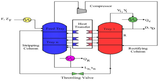
Figure 1.
Heat-integrated distillation column.
In distillation processes, accurate and timely measurement of top and bottom product compositions is essential for effective closed-loop control. However, direct online composition measurements typically obtained via gas chromatographs are often constrained by high costs, slow sampling rates, and very long time delays caused by sampling and analysis procedures. These limitations hinder real-time feedback, leading to control delays, reduced product quality, and inefficient energy use. To overcome these challenges, soft sensors are widely employed to estimate product compositions using easily measurable process variables such as tray temperatures. This study presents the first application of BiLSTM networks for soft sensing of top and bottom product compositions in a HIDiC. The proposed BiLSTM-based model captures the system’s nonlinear and dynamic behavior with high accuracy, enabling real-time composition estimation in a highly complex and thermally coupled distillation process. To demonstrate the effectiveness of the proposed approach, BiLSTM performance is systematically compared with traditional models, including PCR and ANNs. This comparison highlights BiLSTM’s superior capability in capturing the nonlinear dynamics of the HIDiC system and delivering more accurate and reliable real-time composition estimates. This marks a significant step in data-driven inferential control of HIDiCs, showcasing the potential of advanced models for handling process complexity and nonlinearity.
2. System Description
The mechanistic nonlinear model of the HIDiC used in this study is adapted from [22]. The column consists of 54 trays, and the mechanistic model is developed following the assumptions of negligible vapor holdup, constant liquid holdup, perfect mixing of liquid and vapor on each tray, instantaneous heat transfer between the rectifying and stripping sections, negligible pressure drop in both sections, and constant latent heat and relative volatility. The nominal operating conditions used in this study are summarized in Table 1, with a reference setpoint of 99.5% for the top composition (benzene) and 0.5% for the bottom composition (toluene) as in [21]. Following the convention for binary distillation columns, the product composition is given in terms of the lighter product (i.e., benzene). The composition for the heavier product, i.e., toluene, can be worked out as 100% minus the lighter product composition.

Table 1.
Steady state operating conditions of the HIDiC.
3. Machine Learning Models
In modern process industries, accurate real-time estimation of key process variables such as product compositions is vital for effective control and optimization. Traditional analytical instruments like gas chromatographs are often limited by high latency, very long delays, and maintenance demands. To overcome these limitations, machine learning (ML) offers a robust data-driven approach for soft sensor development, enabling the indirect estimation of hard-to-measure variables using readily available process data. This section outlines the architecture and implementation of ML-based soft sensor models for estimating the top and bottom compositions in a HIDiC.
A dataset comprising 3000 samples of tray temperature profiles and associated top and bottom product compositions was generated through dynamic simulation of a HIDiC system implemented in MATLAB (Version 2022a). The simulation was initialized from a steady-state solution obtained under nominal operating conditions and then executed dynamically over 3000 min. Tray temperatures were recorded at 1 min intervals, offering sufficient temporal resolution to capture transient behaviors while maintaining manageable data volume. To simulate realistic operational disturbances, step changes of +15% were applied to the feed composition variable at approximately 400, 1500, and 2000 min. These changes reflect common feedstock variability and were essential for eliciting representative dynamic responses in the column, particularly in tray temperatures and product compositions. A fixed solver time step, significantly smaller than the sampling interval, was employed to ensure numerical stability during the simulation. Following simulation, tray temperatures and composition data were down-sampled to 1 min intervals. To emulate sensor noise, zero-mean Gaussian noise with a standard deviation of 0.1% of the tray temperature value was added to all tray temperature signals. Additionally, zero-mean Gaussian noise with a standard deviation of 0.03% of the nominal composition value was added to the top and bottom product compositions to account for measurement uncertainty. Finally, all input (tray temperatures) and output (compositions) variables were standardized using their respective means and standard deviations to improve model convergence and ensure consistent feature scaling across all soft sensor modeling approaches.
To analyze sensor development, PCR-, ANN-, and BiLSTM-based sensors were developed and evaluated. To ensure a fair and consistent comparison, all three models were trained and tested using the same dataset, with tray temperature profiles as input features and the corresponding product compositions as target outputs. Figure 2 shows the block diagram of the sensor development process using the tray temperature data. The dataset consists of 3000 samples, each representing a snapshot of tray temperature profiles paired with corresponding product composition measurements. The dataset was split into 80% training data (2400 samples) and 20% testing data (600 samples). A 5-fold cross-validation was performed on the training data, using 1920 samples for training and 480 samples for validation in each fold. The final model performance was evaluated on the independent test set, ensuring that the PCR, ANN, and BiLSTM models were trained and validated on the same partitions to maintain consistency in performance evaluation.
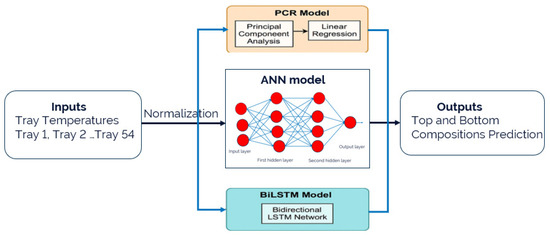
Figure 2.
Block diagram of linear and nonlinear soft sensors.
The inputs to the PCR model consisted of 54 tray temperatures collected from dynamic simulations of the HIDiC system. These inputs were standardized using z-score normalization. PCA was applied to reduce the dimensionality of the input data before regression. Instead of selecting the number of principal components based solely on a retained variance threshold (e.g., ≥99%), which may not yield optimal predictive performance, cross-validation was employed to determine the number of components that minimized the prediction error in the PCR model. Based on the 5-fold cross-validation results using MSE as the performance metric, the optimal number of principal components (PCs) was determined to be 28 for the top composition and 26 for the bottom composition. These values correspond to the lowest validation MSE values observed across the cross-validation folds, indicating that they offer the best generalization performance for their respective PCR models.
A linear regression model was then fitted to the principal components to estimate the top and bottom compositions.
The soft sensor model estimates the product compositions at time t based on the corresponding tray temperature measurements at that same time. The PCR estimation model can be expressed as follows:
where y(t) denotes the product composition at time t, T1(t) to (t) represent the temperatures of trays 1 to 54 respectively, θ1 to are the model parameters, and t indicates the discrete time step. The full set of PCR model coefficients for both the top and bottom composition models is given in the Appendix A.
3.1. Artificial Neural Network
To model the nonlinear relationship between tray temperatures and product compositions in the HIDiC, a feedforward ANN was developed using supervised learning. The structure of the network is illustrated in Figure 3. The model inputs are standardized tray temperature profiles that are mapped to the corresponding top and bottom compositions. All inputs and targets were normalized to have zero mean and unit variance. The optimal size of the ANN model was determined through empirical testing by evaluating various architectures with different numbers of hidden neurons. In Figure 4 and Table 2, [10] represents one hidden layer with 10 hidden neurons and [20,10] represents two hidden layers with 20 neurons in the fist hidden layer and 10 neurons in the second hidden layer. As shown in Figure 4 and Table 2, model performance improves with increased network size up to the [20,10] configuration. Beyond this point, further complexity, ([50,20]), did not significantly enhance accuracy. Therefore, the [20,10] structure was selected as the final ANN model due to its favorable trade-off between accuracy and complexity. In terms of activation functions, the tangent sigmoid (tansig) function was used in the first hidden layer to model the input nonlinearity, while the logarithmic sigmoid (logsig) was employed in the second hidden layer to enhance nonlinear representation. The output layer utilized a linear (purelin) activation function, which is appropriate for continuous regression tasks such as composition estimation.
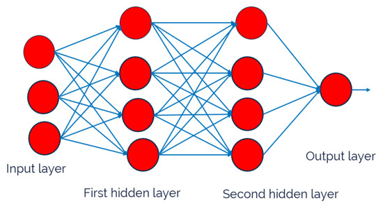
Figure 3.
The block diagram of ANN structure.
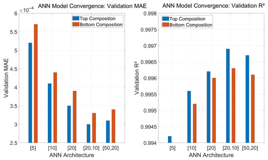
Figure 4.
Validation performance of different ANN architectures for top and bottom composition prediction.
Table 2.
Validation performance of different ANN architectures for top and bottom composition prediction.
To further improve generalization and mitigate overfitting, Bayesian regularization (trainbr) was selected as the training algorithm. This method automatically penalizes overly complex models by adjusting the effective number of parameters during training. The training was configured for up to 1000 epochs, with a minimum gradient threshold of 1 × 10⁻⁷, and incorporated an early stopping criterion triggered after 10 consecutive validation failures (max_fail = 10). A small regularization parameter (0.01) was also applied to encourage smoother model outputs. To ensure reproducibility, the network weights were initialized with fixed random seeds, and training was carried out using MATLAB’s train function. This carefully tuned configuration demonstrated robust predictive performance, as detailed in Section 4.
Figure 4 illustrates the model cross-validation performance of various ANN architectures evaluated during the development of the soft sensor models for top and bottom composition prediction in the HIDiC system. The left panel presents the validation mean absolute error (MAE), while the right panel shows the corresponding coefficient of determination (R2) for different architectures. The tested configurations include both shallow and deeper networks, ranging from a single hidden layer with 5 to 20 neurons to two hidden layers with up to 50 and 20 neurons in the first and second hidden layers respectively. As shown, the validation MAE decreases consistently as the model complexity increases from [5] to [20,10], indicating improved prediction accuracy. Beyond this point, further increases in the number of hidden neurons, e.g. ([50,20]), do not result in significant performance gains and, in some cases, lead to marginal degradation. A similar trend is observed in the R2 values, where the [20,10] architecture achieves the highest accuracy for both top and bottom compositions. These results confirm that the [20,10] architecture offers an optimal balance between model complexity and predictive performance. The clear plateauing of both MAE and R2 beyond this point serves as evidence of model convergence, justifying its selection as the final ANN structure used in this study.
Figure 4 shows that the [20,10] structure achieves the lowest MAE and highest R2 for both outputs, indicating optimal predictive performance. Performance plateaus beyond this point, confirming model convergence.
3.2. Bidirectional Long Short-Term Memory
To enhance the learning of temporal patterns in tray temperature data, a BiLSTM network was employed to estimate the top and bottom compositions in the HIDiC. Unlike standard LSTM, the BiLSTM processes input sequences in both forward and backward directions, simultaneously capturing past and future context. This bidirectional learning capability enhances prediction accuracy, especially under dynamic and transient conditions. Figure 5 shows the architecture of the BiLSTM. Standardized temperature sequences were used as inputs, and the model was trained using a sequence-to-one mapping strategy for real-time soft sensing applications. The BiLSTM network architecture was designed to learn the nonlinear and temporal dependencies between tray temperature profiles and product compositions in the HIDiC system. The input data were structured as sequences of length 10, selected through empirical evaluation to provide sufficient historical context for accurate prediction while maintaining computational tractability. Each input sequence captured 10 consecutive time steps of 54 standardized tray temperatures, and the corresponding target was the standardized composition at the subsequent time step.
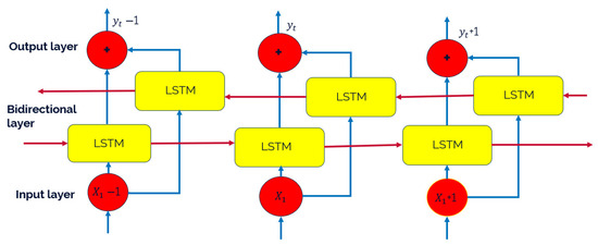
Figure 5.
The architecture of BiLSTM.
The BiLSTM model was empirically tuned by testing multiple architectures with different hidden unit sizes, specifically 20, 50, 100, and 150. In Figure 6 and Table 3, [20] represents 20 hidden units. As shown in Figure 6 and Table 3, validation performance improves with increasing network size up to 100 units. Beyond this point, further increases yields marginal or no gains, indicating convergence. The architecture with 100 hidden units was therefore selected as the final model configuration. The output from the BiLSTM layer was passed through a fully connected layer and a regression output layer, optimized using mean squared error (MSE) loss. Training was carried out using the Adam optimizer with a learning rate of 0.005, a maximum of 200 epochs, and a gradient threshold of 1, which were determined through manual tuning to achieve reliable convergence without overfitting. This architecture and training setup were found to consistently produce accurate and robust predictions for product composition, as confirmed by the results presented in Section 4.
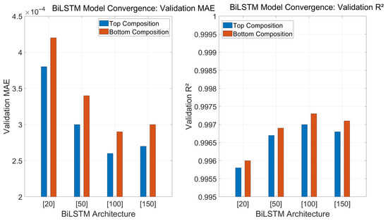
Figure 6.
Validation performance of different BiLSTM architectures for top and bottom composition prediction.
Table 3.
Validation performance of different BiLSTM architectures for top and bottom composition prediction.
Figure 6 summarizes the validation performance of different BiLSTM architectures for top and bottom composition prediction. As the number of hidden units increases from 20 to 100, MAE decreases and R2 improves, indicating better prediction accuracy. The architecture with 100 hidden units yields the best overall performance for both outputs. Increasing to 150 units offers no substantial improvement and may slightly degrade performance, confirming convergence at 100 units. This configuration was therefore selected as the optimal BiLSTM model for this study.
4. Results and Discussion
This section presents the results and analyzes the performance of PCR, ANN, and BiLSTM data-driven models developed to estimate the top and bottom product compositions in a HIDiC. A dataset with 3000 samples of tray temperatures and the top and bottom compositions was used, and the data were split into 80% for training (2400 samples) and 20% for testing (600 samples). A five-fold cross-validation was performed on the training data, using 1920 samples for training and 480 samples for validation in each fold. Standard metrics such as the MAE, MSE, and R2 were used to evaluate the performance of the models.
Figure 7 and Figure 8 show the performance of the PCR model in predicting the top and bottom product compositions. Following the convention for binary distillation columns, the product composition is given in terms of the lighter product (i.e., benzene). The composition for the heavier product, i.e., toluene, can be worked out as 100% minus the lighter product composition. The upper subplot illustrates a close agreement between the actual compositions values and those predicted by the PCR model across the entire simulation time. The predicted trajectory successfully tracks the major dynamic trends and steady-state regions, including sharp drops and gradual recoveries, indicating the model’s effectiveness in capturing underlying system behavior.
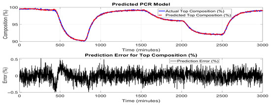
Figure 7.
Performance of the PCR model in predicting top product (benzene) composition.
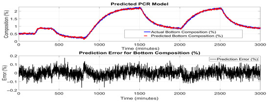
Figure 8.
PCR model performance for predicting bottom product (toluene) composition.
However, as shown in the lower subplot of the figures, the prediction errors fluctuate over time, particularly in dynamic transition regions around 400–1000 and 1800–2500 min, where rapid changes in composition occur. The error mostly remains within ±0.5%, which is reasonably acceptable for many control applications, considering that PCR is a linear method based on a reduced set of principal components. The slight increase in prediction error during highly dynamic intervals can be attributed to PCR’s inherent limitations in modeling nonlinear relationships and temporal dependencies within time-series data. PCR relies on the projection of high-dimensional input features, tray temperatures, into a lower-dimensional space, which may discard some nonlinear dynamics crucial for precise tracking.
Figure 9 and Figure 10 show the performance of the ANN model in predicting the top and bottom product compositions in the HIDiC. The upper subplots illustrate an excellent match between the actual top and bottom composition values and the ANN model predicted values. The model predictions align closely with the true values across both steady-state regions and periods of dynamic change, demonstrating the ANN’s capability to learn and represent complex nonlinear relationships in the process data. The lower subplots in Figure 9 and Figure 10 present the prediction errors over time. The errors remain tightly bounded, typically within ±0.3%, which confirms the model’s robustness and suitability for real-time estimation tasks. Compared to PCR, the ANN model maintains more consistent accuracy, even in dynamic regions of the process such as between 400 and 1000 min and between 1800 and 2500 min, where composition changes rapidly due to operational transitions.
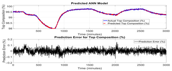
Figure 9.
ANN model performance for predicting top product (benzene) composition.
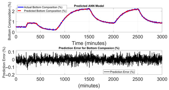
Figure 10.
ANN model performance for predicting bottom product (toluene) composition.
The ANN’s superior performance highlights its strength in capturing nonlinear and multivariate dependencies among the input and output variables. Unlike PCR, which reduces dimensionality at the expense of potentially discarding important dynamic features, the ANN uses fully connected layers and nonlinear activation functions to retain and learn complex mappings from model inputs to outputs.
Figure 11 and Figure 12 illustrate the performance of the BiLSTM network in predicting the top and bottom product compositions of the HIDiC. In the upper subplots, the predicted values closely follow the actual product compositions over the entire simulation period. The BiLSTM model accurately captures dynamic trends, including rapid increases, plateaus, and sharp declines, highlighting its strength in modeling complex time-dependent behaviors. The lower subplots in the figures show the prediction errors at different samples. The error remains well within ±0.1% for most of the time, with minimal spikes even during periods of sudden changes in composition. This tight error distribution indicates a significant enhancement in prediction precision compared to both PCR and ANN models. Due to the use of sequence-based learning, predictions begin only after the initial window length (10 samples), which shifts the alignment of actual and predicted signals. This design ensures that the model captures temporal context but results in plots that do not start from the very first time point. Nonetheless, the prediction accuracy stabilizes quickly after this initial offset. Rolling average plots for both training and testing predictions indicate that the model performs with low bias and moderate noise, especially in high-variation regions of the dataset. This is consistent with the high R2 value (0.9991), confirming the model’s ability to explain most of the variance in the output.
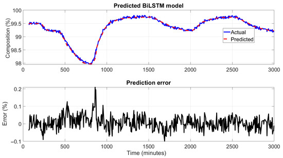
Figure 11.
BiLSTM model performance for predicting top product (benzene) composition.
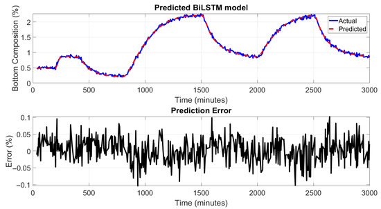
Figure 12.
BiLSTM model performance for predicting bottom product (toluene) composition.
The superior performance of the BiLSTM model can be attributed to its inherent ability to capture long-range temporal dependencies by processing input sequences in both forward and backward directions. Unlike traditional ANN models, which lack memory of previous time steps, BiLSTM networks are well-suited for sequence prediction tasks in this dynamic process where current states are influenced by past trends and inputs.
To assess the effectiveness of the proposed BiLSTM model, its performance is further compared to ANN and PCR via the MAE, MSE, and R2. Table 4 summarizes the comparative results for both top and bottom product compositions computed on training and testing datasets. For the top composition, while all models performed well, the BiLSTM model achieved the highest R2 of 0.9980, indicating a better fit to the actual top composition than both PCR and ANN. The BiLSTM model’s superior R2 suggests that it captured the system’s underlying nonlinear dynamics more comprehensively. The PCR model, while being significantly simpler and faster to train, underperformed due to its inherent linearity and lack of temporal modeling capability. This confirms that deep learning models, especially BiLSTM, are more appropriate for time-dependent chemical process modelling. While the BiLSTM model achieves the highest prediction accuracy among the evaluated approaches, it also incurs more computational costs in terms of training time. As presented in Table 4 and illustrated in Figure 13 above, the PCR model is computationally inexpensive and trains almost instantaneously. In contrast, the ANN and the BiLSTM models demand more training time due to their increased architectural complexity and larger number of trainable parameters.
Table 4.
Model performance metrics for top and bottom composition prediction.
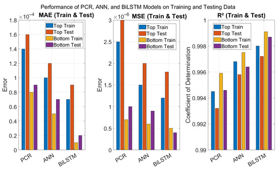
Figure 13.
Bar chat of performances of three soft sensor models.
For the bottom composition, the BiLSTM again outperforms the other models, achieving the highest R2 of 0.9991. The ANN model comes close in performance, but BiLSTM offers better generalization and temporal tracking, as seen in the prediction plots and residual errors. PCR’s performance on the bottom composition is relatively acceptable but again limited by its linear assumptions and static nature, which restrict its ability to adapt to process dynamics. PCR is efficient for quick deployment and interpretable modeling but lacks the ability to handle nonlinear and dynamic behavior. ANN offers better nonlinear modeling than PCR but lacks memory and struggles with time-sequenced data unless explicitly structured with delays. BiLSTM provides the most accurate and consistent predictions due to its bidirectional memory mechanism, which captures both forward and backward dependencies in process variables. These results strongly justify the use of BiLSTM networks as the preferred soft sensor architecture for real-time monitoring and control in HIDiC systems.
Across all the evaluation metrics, the BiLSTM models consistently outperform the ANN and PCR models, confirming their ability to model complex and dynamic relationships in the data as showed in Figure 13. For the training set, BiLSTM models achieve the lowest MAE values of 0.00007 (top) and 0.00001 (bottom), and the lowest MSE values of 1.2 × 10⁻⁶ and 5.0 × 10⁻⁷, respectively. In terms of R2, BiLSTM models record 0.9980 (top) and 0.9991 (bottom), indicating a very good fit. On the testing set, BiLSTM models maintain their superior performance, with MAEs of 0.00009 (top) and 0.00002 (bottom), and R2 values of 0.9972 (top) and 0.9987(bottom). This strong generalization capability is critical for real-time control applications. The ANN models perform slightly below the BiLSTM models but still significantly better than the PCR models in all cases. PCR, being a linear method, shows the lowest R2 and highest errors, particularly for the top composition prediction. These results emphasize the inherent trade-off between model accuracy and computational efficiency, with BiLSTM providing superior predictive performance with more computational effort. Figure 14 presents the training times for the three models, PCR, ANN, and BiLSTM, measured in seconds on the same training dataset. The figure clearly demonstrates the trade-off between computational cost and model complexity. The PCR model, being the simplest with a linear structure, requires minimal training time (0.3 s), making it highly efficient but less flexible. The ANN model, with its nonlinear structure and greater number of parameters, necessitates a moderate increase in training time (12.5 s). The BiLSTM model, characterized by its deep recurrent layers and capacity to capture temporal dependencies, demands the most computational effort, taking roughly 86.5 s to train. While the BiLSTM delivers superior predictive performance, as shown in Figure 11 and Figure 12, this comes at a significantly higher computational cost. These results underscore the important balance between accuracy and efficiency, emphasizing that model selection should consider not only predictive capability but also resource constraints and application requirements, especially in real-time or large-scale scenarios.
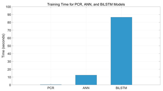
Figure 14.
Comparison of computation time of three soft sensor models.
In summary, this comparison demonstrates that deep learning models, particularly BiLSTM, are the most effective for developing accurate soft sensors in heat-integrated distillation systems.
5. Conclusions
This study presents the development and comparative evaluation of data-driven soft sensor models for real-time estimation of top and bottom product compositions in a HIDiC. The PCR, ANN, and BiLSTM models were designed using tray temperatures as model inputs. These models were investigated, and their performance was evaluated. It is shown that the BiLSTM architecture consistently outperforms the others, achieving the lowest MAE and MSE, and the highest R2 scores for both top and bottom composition estimations. Its ability to learn temporal dependencies in both forward and backward directions results in smoother and more accurate predictions, making it highly suitable for deployment in real-time estimation and control. While PCR offers a simple and interpretable baseline, it struggles to capture nonlinear and dynamic behaviors due to its linear structure. The ANN model improves upon PCR by capturing nonlinear relationships but still lacks the temporal memory necessary for tracking complex transients. In contrast, BiLSTM provides superior dynamic tracking, low error margins, and robust generalization. Despite the increased computational burden associated with BiLSTM due to its sequential training and parameter complexity, the results affirm that recurrent deep learning architectures like BiLSTM hold significant promise for soft sensing applications in complex chemical processes like HIDiCs, where precise and real-time composition estimation is critical. Future work will focus on integrating the trained BiLSTM soft sensor with advanced control schemes for online composition measurement and control in HIDiC systems.
Author Contributions
Conceptualization, N.M.T. and J.Z.; methodology, N.M.T. and J.Z.; software, N.M.T. and J.Z.; validation, N.M.T.; formal analysis, N.M.T.; investigation, N.M.T.; resources, J.Z. and M.A.; data curation, N.M.T. and J.Z.; writing—original draft preparation, N.M.T.; writing—review and editing, J.Z. and M.A.; visualization, N.M.T.; supervision, J.Z. and M.A.; project administration, J.Z. and M.A. All authors have read and agreed to the published version of the manuscript.
Funding
This work is sponsored by the Petroleum Technology Development Fund, Nigeria, and supported by Abubakar Tafawa Balewa University, Bauchi, Nigeria.
Data Availability Statement
Data will be made available on request.
Conflicts of Interest
The authors declare no conflict of interest.
Abbreviations
The following abbreviations are used in this manuscript:
| ANN | Artificial Neural Network |
| BiLSTM | Bidirectional Long Short-Term Memory |
| BUMDA | Binary Update Multi-Decision Algorithm |
| CO2 | Carbon Dioxide |
| HIDiC | Heat-Integrated Distillation Column |
| MAE | Mean Absolute Error |
| MILP | Mixed-Integer Linear Programming |
| MINLP | Mixed-Integer Nonlinear Programming |
| MSE | Mean Squared Error |
| MV | Manipulated Variable |
| PCA | Principal Component Analysis |
| PCR | Principal Component Regression |
| PCs | principal components |
| PSO | Particle Swarm Optimization |
| R2 | Coefficient of Determination |
| ReLU | Rectified Linear Unit |
| RMSE | Root Mean Squared Error |
| TAC | Total Annual Cost |
| TWPM | Transient Wave Propagation Model |
| WPM | Wave Propagation Model |
Appendix A
This appendix presents the PCR model coefficients for predicting top and bottom product compositions in a HIDiC, using tray temperatures as inputs. Table A1 and Table A2 give the model parameters for the top and bottom compositions, respectively.
Table A1.
PCR model coefficients for top product composition.
Table A1.
PCR model coefficients for top product composition.
| Tray No. | Coefficient | Tray No. | Coefficient | Tray No. | Coefficient |
|---|---|---|---|---|---|
| 1 | −0.066334 | 19 | 0.028730 | 37 | −0.000823 |
| 2 | −0.199253 | 20 | 0.005451 | 38 | −0.007860 |
| 3 | −0.250045 | 21 | −0.002330 | 39 | 0.005594 |
| 4 | −0.235453 | 22 | −0.018362 | 40 | −0.028649 |
| 5 | −0.211019 | 23 | −0.030797 | 41 | −0.008952 |
| 6 | −0.192612 | 24 | −0.034408 | 42 | 0.001113 |
| 7 | −0.127935 | 25 | −0.036235 | 43 | −0.010895 |
| 8 | −0.073083 | 26 | −0.026121 | 44 | 0.003418 |
| 9 | −0.035022 | 27 | −0.029371 | 45 | −0.004782 |
| 10 | −0.005901 | 28 | 0.022753 | 46 | −0.004325 |
| 11 | 0.008731 | 29 | 0.035445 | 47 | 0.000357 |
| 12 | 0.025629 | 30 | 0.031885 | 48 | −0.000445 |
| 13 | 0.038951 | 31 | 0.034885 | 49 | −0.004172 |
| 14 | 0.040749 | 32 | 0.047070 | 50 | −0.001687 |
| 15 | 0.052568 | 33 | 0.047657 | 51 | 0.000544 |
| 16 | 0.058263 | 34 | 0.034723 | 52 | 0.002290 |
| 17 | 0.047005 | 35 | 0.028097 | 53 | 0.003309 |
| 18 | 0.035033 | 36 | 0.008015 | 54 | 0.000688 |
Table A2.
PCR model coefficients for bottom product composition.
Table A2.
PCR model coefficients for bottom product composition.
| Tray No. | Coefficient | Tray No. | Coefficient | Tray No. | Coefficient |
|---|---|---|---|---|---|
| 1 | 0.000004 | 19 | −0.000183 | 37 | −0.000079 |
| 2 | −0.000011 | 20 | −0.000199 | 38 | −0.000152 |
| 3 | 0.000007 | 21 | −0.000204 | 39 | −0.000219 |
| 4 | −0.000035 | 22 | −0.000160 | 40 | −0.000359 |
| 5 | −0.000004 | 23 | −0.000150 | 41 | −0.000383 |
| 6 | −0.000026 | 24 | −0.000097 | 42 | −0.000512 |
| 7 | 0.000088 | 25 | 0.000050 | 43 | −0.000580 |
| 8 | 0.000079 | 26 | 0.000213 | 44 | −0.000641 |
| 9 | 0.000060 | 27 | 0.000160 | 45 | −0.000898 |
| 10 | 0.000125 | 28 | 0.000108 | 46 | −0.000806 |
| 11 | 0.000135 | 29 | 0.000065 | 47 | −0.000641 |
| 12 | 0.000355 | 30 | 0.000144 | 48 | −0.000493 |
| 13 | 0.000191 | 31 | 0.000166 | 49 | −0.000404 |
| 14 | 0.000029 | 32 | 0.000312 | 50 | −0.000383 |
| 15 | −0.000022 | 33 | 0.000277 | 51 | −0.000333 |
| 16 | −0.000072 | 34 | 0.000165 | 52 | −0.000252 |
| 17 | −0.000089 | 35 | 0.000104 | 53 | −0.000198 |
| 18 | −0.000145 | 36 | −0.000013 | 54 | −0.000272 |
References
- Tahir, N.M.; Zhang, J.; Armstrong, M. Control of Heat-Integrated Distillation Columns: Review, Trends, and Challenges for Future Research. Processes 2024, 13, 17. [Google Scholar] [CrossRef]
- Bisgaard, T.; Skogestad, S.; Huusom, J.K.; Abildskov, J. Optimal Operation and Stabilizing Control of the Concentric Heat-Integrated Distillation Column. IFAC-Pap. Online 2016, 49, 747–752. [Google Scholar] [CrossRef][Green Version]
- Cong, H.; Liu, Y. An adaptive set-point correction method based on temperature profile movement for high-purity heat-integrated distillation columns. Chin. J. Chem. Eng. 2020, 28, 157–167. [Google Scholar]
- He, X.; Cong, H.; Yang, C.; Liu, Y. Dynamic controllability of various heat-integrated pressure swing distillation processes. Chin. J. Chem. Eng. 2020, 28, 228–237. [Google Scholar]
- Babaie, A.; Esfahany, M.N. Energy and cost reduction in reactive distillation–pervaporation hybrid process using internally heat integrated distillation column. Chem. Eng. Process.-Process Intensif. 2020, 149, 107854. [Google Scholar]
- Cong, H.; Wu, X.; Liu, Y. Profile pattern-based modeling and control for heat integrated distillation columns. Chem. Eng. Process.-Process Intensif. 2021, 163, 108385. [Google Scholar]
- Jaleel, H.U.; Shah, H.A.; Khan, M.A.; Ali, H. Soft sensor design for heat-integrated distillation columns using support vector regression and swarm-based optimization. Energy Rep. 2022, 8, 3427–3437. [Google Scholar]
- Cheng, Y.; Fan, Y.; Zhang, P.; Yuan, Y.; Li, J. Design and parameter tuning of active disturbance rejection control for uncertain multivariable systems via quantitative feedback theory. ISA Trans. 2023, 141, 288–302. [Google Scholar] [CrossRef] [PubMed]
- Cong, L.; Liu, X. Temperature profile movement investigation and application to a control scheme with corrected set-point for a heat integrated distillation column. Chem. Eng. Process.-Process Intensif. 2020, 147, 107710. [Google Scholar] [CrossRef]
- Cong, L.; Xu, L.; Liu, X. Adaptive Temperature Control for Distillation Columns Based on Relative Stability in the Profile Pattern. Ind. Eng. Chem. Res. 2021, 60, 514–527. [Google Scholar] [CrossRef]
- Jaleel, E.A.; Anzar, S.M.; Rehannara Beegum, T.; Mohamed Shahid, P.A. System identification and control of heat integrated distillation column using artificial bee colony-based support vector regression. Chem. Eng. Commun. 2022, 209, 1377–1396. [Google Scholar] [CrossRef]
- Mancera-Apolinar, J.A.; Mendoza, D.F.; Riascos, C.A.M. Preliminary Conceptual Design of a Distillation Column with Energy Integration (HIDiC). Chem. Eng. Trans. 2023, 100, 733–738. [Google Scholar] [CrossRef]
- Shahana, K.S.P.; Jaleel, A. Neural Network for Identification of Heat Integrated Distillation Column. In Proceedings of the 2020 International Conference on Futuristic Technologies in Control Systems & Renewable Energy (ICFCR), Malappuram, India, 23–24 September 2020; IEEE: New York, NY, USA, 2020. [Google Scholar]
- Yuan, X.F.; Ge, Z.Q.; Huang, B.; Song, Z.H.; Wang, Y.L. Semi supervised JITL framework for nonlinear industrial soft sensing based on locally semi-supervised weighted PCR. IEEE Trans. Ind. Inf. 2017, 13, 532–541. [Google Scholar] [CrossRef]
- Tan, X.Y.; Guo, W.; Liu, R.R.; Pan, T.H. A data-driven soft-sensing approach using probabilistic latent variable model with functional data framework. Trans. Inst. Meas. Control 2024, 46, 913–926. [Google Scholar] [CrossRef]
- Kaneko, H.; Funatsu, K. Application of online support vector regression for soft sensors. AIChE J. 2014, 60, 600–612. [Google Scholar] [CrossRef]
- Alhajeri, M.S.; Ren, Y.; Ou, F.Y.; Abdullah, F.; Christofides, P. Model predictive control of nonlinear processes using transfer learning-based recurrent neural networks. Chem. Eng. Res. Des. 2024, 205, 1–12. [Google Scholar] [CrossRef]
- Al Kalbani, F.; Zhang, J. Inferential Composition Control of a Distillation Column Using Active Disturbance Rejection Control with Soft Sensors. Sensors 2023, 23, 1019. [Google Scholar] [CrossRef] [PubMed]
- Zhou, X.; Song, E.; Wang, M.; Wang, E. Dynamic Temperature Control of Dividing Wall Batch Distillation with Middle Vessel Based on Neural Network Soft-Sensor and Fuzzy Control. Chin. J. Chem. Eng. 2025, 79, 200–211. [Google Scholar] [CrossRef]
- Tahir, N.M.; Zhang, J.; Armstrong, M. Advancing control paradigms in heat-integrated distillation columns: An MPC perspective. In Proceedings of the 29th International Conference on Automation and Computing (ICAC), Sunderland, UK, 28–30 August 2024; IEEE: New York, NY, USA, 2024. [Google Scholar]
- Tahir, N.M.; Zhang, J.; Armstrong, M. Genetic Algorithm Optimization based Control for Heat Integrated Distillation Column. In Proceedings of the 22nd International Learning and Technology Conference (L&T), Jeddah, Saudi Arabia, 15–16 January 2025; IEEE: New York, NY, USA, 2025; Volume 22, pp. 77–82. [Google Scholar]
- Bisgaard, T.; Huusom, J.K.; Abildskov, J. A Modeling Framework for Conventional and Heat Integrated Distillation Columns. IFAC Proc. Vol. 2013, 46, 373–378. [Google Scholar] [CrossRef]


Disclaimer/Publisher’s Note: The statements, opinions and data contained in all publications are solely those of the individual author(s) and contributor(s) and not of MDPI and/or the editor(s). MDPI and/or the editor(s) disclaim responsibility for any injury to people or property resulting from any ideas, methods, instructions or products referred to in the content. |
© 2025 by the authors. Licensee MDPI, Basel, Switzerland. This article is an open access article distributed under the terms and conditions of the Creative Commons Attribution (CC BY) license (https://creativecommons.org/licenses/by/4.0/).