Abstract
The design of ventilation and air conditioning systems in university classrooms is paramount to ensure students’ correct number of air changes per hour and an optimal thermal profile for their comfort. With the spread of the COVID-19 virus, these systems will inevitably need to evolve to cope with the current virus and any new airborne pathogens. The aim of this study is to analyze the quality of the ventilation system and the importance of the use of PPE in Lecture Hall C of the University of Naples Federico II compared to the premises in Piazzale Tecchio. After dimensioning the lecture theatre with the Autodesk software AutoCAD 2021, CFD simulations were carried out with the Computational Fluid Dynamics program Ansys 2021 R2. To study the trajectory of virus droplets released by a potentially infected student in the center of the classroom, the multispecies model was used, with carbon dioxide serving as the tracer gas for the virus cloud. After determining the CO2 contour zones at fifteen-minute intervals for a total duration of two hours, the probability of infection was calculated using the Wells–Riley equation.
1. Introduction
Indoor air quality control is an important issue worldwide because, according to the World Health Organisation, 4.6 million people die every year from diseases directly linked to poor air quality [1]. The COVID-19 pandemic has further emphasized improving indoor air quality to reduce the risk of airborne infection. By properly designing heating, ventilation and air conditioning (HVAC) systems, it is possible to optimize ventilation in an indoor space to reduce the risk of infectious exposure while ensuring a certain level of safety for all people staying in that space, even for extended periods of time [2].
There are several methods to improve indoor air quality by HVAC operation, each with different advantages and disadvantages. Guo et al. (2021) summarized and compared HVAC operating guidelines during the COVID-19 pandemic for buildings in different countries [3]. Based on this research, the following common strategies were developed: (1) increasing the outdoor air supply as much as possible, (2) running the HVAC system longer to eliminate the persistent virus, and (3) improving recirculating air filtration. Increasing the outdoor air supply can dilute the virus concentration indoors without the need to purchase new equipment. However, increasing the outdoor air supply rate can significantly increase energy consumption for cooling/heating if the outdoor air temperature differs significantly from the set room temperature. Increasing the supply air rate can affect thermal comfort, as most HVAC systems are not designed for higher outside air rates than the design values. Furthermore, extending the operating time of the HVAC system, e.g., by running it for longer before or after occupants arrive, can help to eliminate persistent viruses in the room.
In order to evaluate the effectiveness of HVAC measures, the spread of virus droplets in a closed environment can be analyzed by particle simulation (discrete phase models) or by tracer gas simulation (species transport). In the simulation with the first discrete approach, the temporal and spatial fate of each particle emitted by a potentially infected person is tracked. The movement of the particles is subject to various forces, including gravitational force, thermophoretic force, Brownian force, and Saffman lifting force. The ability of the particles to settle on surfaces, resuspend from surfaces, vaporize, coagulate, and change phase should also be taken into account [4]. Solving the discrete phase equations by including the rigorous characterization of the mentioned phenomena involves a high computational cost, as well as in the case of near-field dispersion [5]. In particular, given the nature of the motion in a closed and ventilated turbulent-type environment, the discretizing elements into which to divide the domain and solve all the balance equations must be of different sizes to capture the vortical nature of the motion (from the Kolmogorov scale to the characteristic size of the domain) [6].
For this reason, a continuous gas tracer approach was adopted, in which the particle population is assimilated to a gas with similar physicochemical properties. The model gas must have properties between the neutral/positive buoyancy behavior of aerosols and the negative buoyancy behavior of large droplets. Previous studies have shown a good fit between the trajectories of the tracer gas and those of the small particles.
Bivolarova et al. (2017) investigated the influence of ventilation speed and free convection flow generated by a heat dummy on the dispersion of tracer gas (N2O) and particles (0.07, 0.7 and 3.5 μm) in a room [7]. The gas and particle concentrations were measured in the main part of the room and in the breathing zone of the dummy. The results showed that the use of tracer gas in the breathing zone of the seated dummy allows reliable prediction of the characteristic dispersion pathways for all three particle types investigated, regardless of the variation in ventilation rate and the presence of objects in the room [7].
Zhang et al. (2009) investigated the contaminant transport in a section of an aircraft cabin where a tracer gas (SF6) and particles (0.7 μm) were released to simulate gaseous and particulate contamination. The results show that the distributions of gaseous and particulate contaminants are similar throughout most of the cabin (with the exception of the area near the ceiling), suggesting that particles of this size behave similarly to the tracer gas [8]. Noakes et al. (2009) experimentally compared the tracer gas technique and the particulate approach to assess the behavior of bioaerosols in hospital isolation rooms where air changes are performed 10 times per hour. Both tracer gas (N2O) and particulate matter (3–5 μm) were released from a heated cylinder simulating a bedridden patient. The results showed that both the N2O tracer gas and the particles well simulated the behavior of bioaerosols [9].
Gao et al. (2007) modeled particle dispersion in a room furnished with a thermal dummy, computer, desk, ceiling lights and a mechanical ventilation system. Particle dynamics was treated using the Eulerian approach in combination with a drift-flux model. It was found that the motion of particles of maximum size 2.5 μm is similar to that of tracer gas [10]. Xiaoping et al. (2011) simulated the spatial distribution of droplets emanating from the breathing activity of two people placed face-to-face in an office as ventilation conditions changed. Particles with sizes of 1, 2, 5 and 10 μm and CO2 as the tracer gas were examined. Results show that the spatial distribution of particles no larger than 2.5 μm is very close to that of the tracer gas [11]. A study by Beato-Arribas et al. (2015) concluded that the distributions of CO2 tracer gas and aerosolized Bacillus bacterium detected within an isolated hospital room in which 12 hourly changes are performed show comparable results [12].
All these studies indicate that the simulation of a tracer gas is sufficiently accurate to study the dispersion of particles larger than 3–5 μm. This size range characterizes most of the droplets released by human respiratory activities; moreover, when the far-field dispersion has to be investigated (distances greater than 1 m from the infected individual), it is reasonable to assume that only the latter remains suspended in air. To the best of our knowledge, few works have been carried out about the effect of PPE, and attention has mainly been focused on near-field dispersion [13,14].
In recent years, school and university classrooms have attracted the attention of several researchers as an environment for COVID-19 transmission among students [15,16,17,18]. In these works, several aspects of COVID-19 transmission were analyzed, such as the effects of installing transparent barriers at student desks, ventilation layout and conditions, relative positions of airflow and infected person and air purifiers. In the period 2021–2023, several other papers were published on the topic investigating the dispersion of the virus in very different enclosed spaces [19,20,21,22].
In most cases, the dispersion of the virus was simulated with the use of a gas tracer, but to the best of our knowledge, no actual evaluation of quantitative risk was carried out based on these CFD results, mostly as a joint function of ventilation and DPI utilization. The aim of this work is to verify and optimize the ventilation system present in a classroom on the engineering campus of the University of Naples Federico II (Classroom C, P.le Tecchio) to minimize the risk of COVID-19 infection.
The scenario that will be simulated is the following: a single infected student exhales virus particles and infects any students and/or teachers present in the classroom.
Under varying ventilation conditions and the presence or absence of the FFP2 mask worn by the infected student, the following five cases will be simulated:
- The ventilation system is on and operating according to current guidelines; the mask is not worn by the infected student.
- The ventilation system was turned off; the mask was not worn by the infected student.
- The ventilation system is on and functioning according to current guidelines; the mask is worn by infected students.
- The ventilation system is on (flow rate tripled); the mask is not worn by the infected student.
- The ventilation system is on (flow rate tripled); the mask is worn by the infected student.
In each case, we considered three different scenarios for the exposed people:
- 6.
- The exposed students and/or teachers are not wearing PPE.
- 7.
- The exposed students and/or teachers are wearing surgical masks.
- 8.
- The exposed students and/or teachers are wearing FFP2 masks.
This paper mainly analyzes the role of personal protective equipment in conjunction with the role of ventilation. After characterizing the temporal and spatial trends of virus concentration using Ansys Fluent 2021 R2 software, the probability of infection is calculated using the Wells–Riley equation. The optimal strategy to prevent an infection is the one that has a lower probability of infection at the defined critical points. The chosen observation time is two hours (the duration of a typical university lecture), and the results are analyzed in 15-min intervals so that a total of eight intervals are available for each scenario presented. The study conducted in the following paper, which deals specifically with the COVID-19 virus, applies more generally to airborne viruses and/or bacteria such as influenza, measles, chickenpox, legionella, tuberculosis, etc.
2. Methodology
2.1. CFD Model: Geometrical Domain
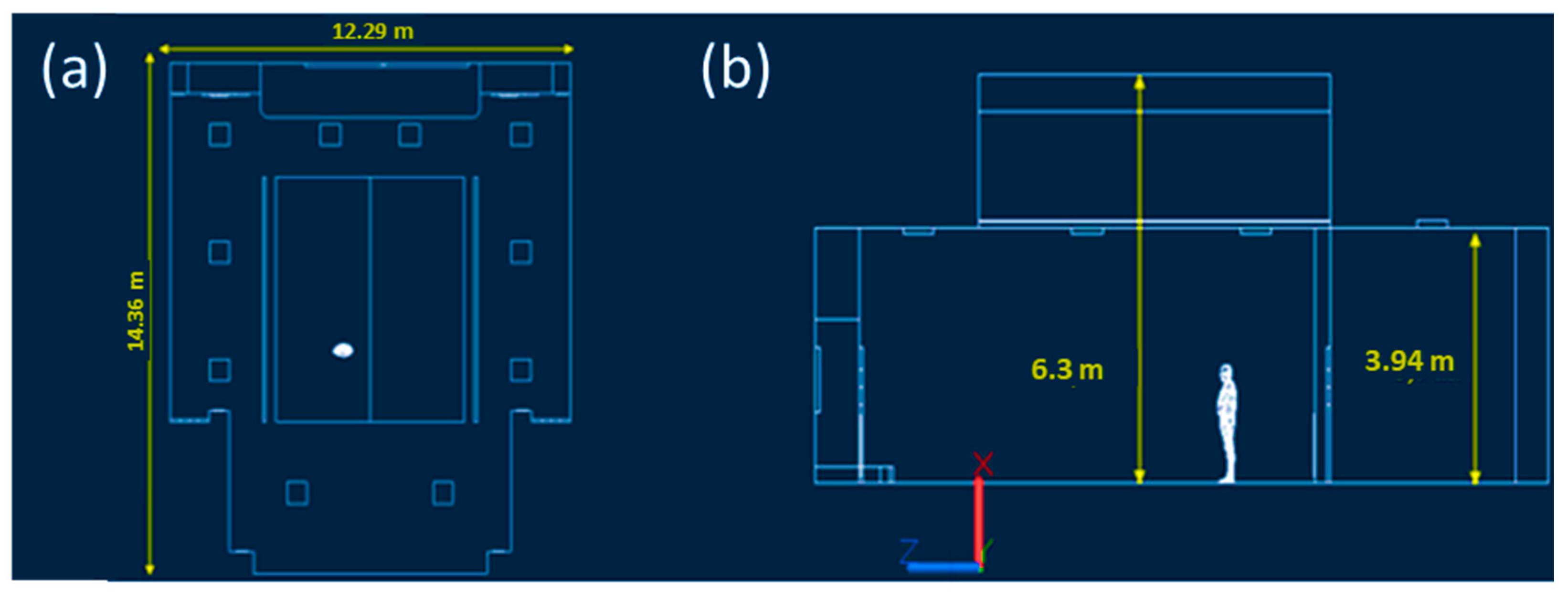
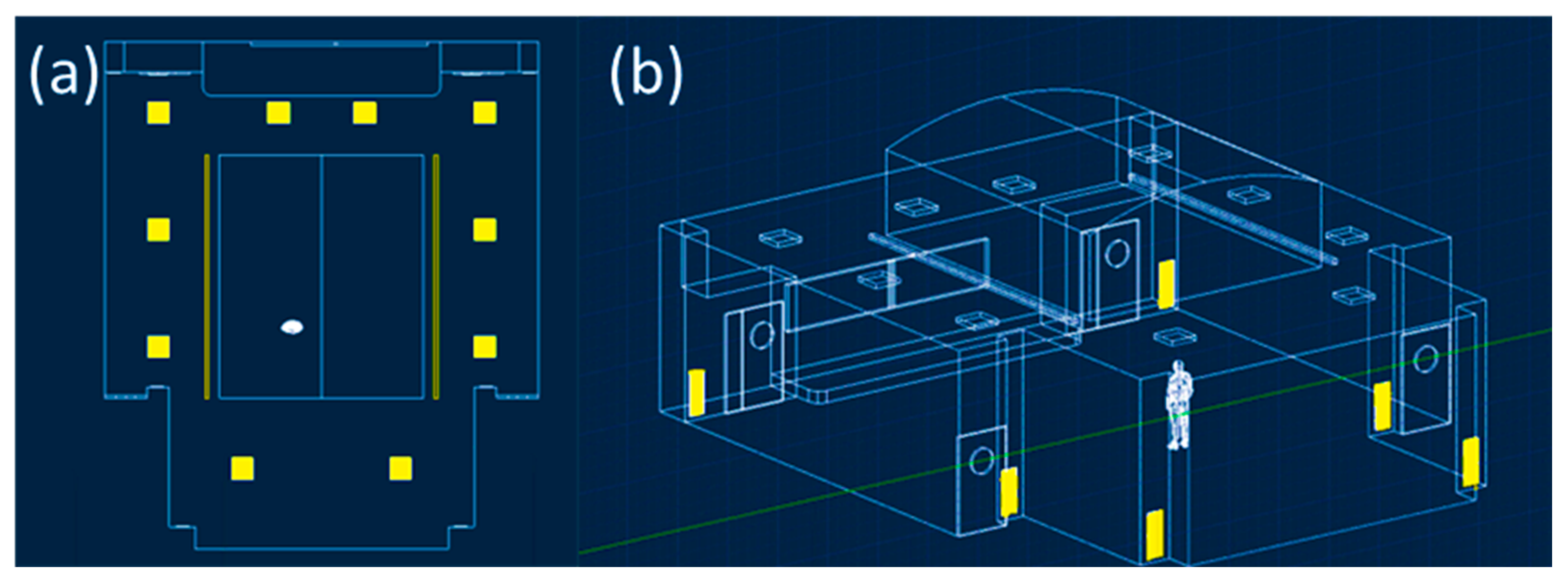
Classroom C was initially dimensioned by direct survey with the Makita LD050P laser meter. As shown in Figure 1, the classroom has a maximum width and length equal to 12.29 m and 14.36 m, the maximum and average wall height dimensioned in Figure 1 are 6.3 m and 3.94 m, for a total classroom volume equal to 696.96 m3. Next, the model was spatially constructed using Autodesk AutoCAD 2021 software. As reported in Figure 1, there are different air supply elements that are better visible and described in Figure 2. The ventilation system is characterized, as shown in Figure 2a, by ten square air supply elements with dimensions of 0.6 m × 0.6 m and two rectangular elements with dimensions of 6.67 m × 0.15 m. The return air characteristic elements, as highlighted in Figure 2b, are six and rectangular in size, equal to 0.96 m × 0.36 m. The guaranteed hourly changes, as shown in the circular issued by the university, are five, and per the current COVID-19 standard, 100% fresh air is provided. Then, the indoor air, once directed to the supply air duct, is expelled to the outside [23]. Noting the geometry and relevant characteristics of the ventilation system, it was possible to calculate the velocity of airflow from the single supply element with a value of 0.3 m/s.
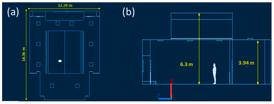
Figure 1.
Characteristic measurements of Classroom C at the University of Naples Federico II. The top view shows maximum width and length (a), the side view shows average and maximum wall height (b) and was drawn with Autodesk Autocad 2021 software.
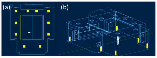
Figure 2.
The twelve characteristic elements of the supply (a) and return elements of the ventilation system (b) were drawn with Autodesk Autocad 2021 software.
2.2. CFD Model: Mesh Building
The AutoCAD file was then imported into Ansys 2021R2 to develop the mesh. Four unstructured meshes were developed; the main properties expressed in a number of nodes, elements and average orthogonal quality are summarized in Table 1. Grid independence tests were performed, and the results are reported in Supplementary Materials.

Table 1.
Comparison of the number of nodes, elements and average orthogonal quality among the used meshes.
2.3. CFD Model: Equations and Boundary Conditions
The CFD model of the dispersion of the SARS-CoV-2 virus within Classroom C was developed under several simplifying assumptions. The infected student releases the virus solely through the process of breathing; other events, such as coughing and/or sneezing, were not considered rare and negligible events compared to the total observation time. Breathing is characterized by three phases: inhalation, exhalation, and pause. Only a single continuous exhalation phase occurs at maximum exhalation velocity (the worst-case scenario). The tracer gas method was adopted, neglecting the particulate nature of the virus and carbon dioxide was used as the tracer gas. CO2 is an excellent biomarker of exhaled breath for risk assessment since it has a density similar to the air-particle cloud of suspended viruses. It is naturally released through exhaled breath along with the virus, and it was already used in previous works [12]. The transient flow of the continuous phase treated as an ideal gas and consisting of two components (air and CO2), was simulated by means of the Ansys Fluent software (version 2021 R2) using the time-averaged Navier–Stokes equations (URANS), the Eulerian approach and implementing the k-ε model as a turbulent sub-model.
where (kg m−3) is the fluid density, (m s−1) is the fluid velocity vector, (Pa) is the static pressure, (Pa) is the stress tensor, and (m s−2) is the gravity vector. With regards to the species transport, Ansys predicts the local mass fraction of the species through the solution of a convection–diffusion equation for the species. The conservation equation takes the following general form:
where (−) is the local mass fraction of CO2, (kg m−2 s−1) is the diffusion flux of CO2 which arises due to gradients of concentration and temperature, (m2 s−1) is the mass diffusion coefficient for CO2, (Pa s) is the turbulent viscosity, (−) is the turbulent Schmidt number, (m2 s−1) is the thermal (Soret) diffusion coefficient, (K) is the absolute temperature.
The average Navier–Stokes equations were discretized using the finite volume method on an unstructured three-dimensional mesh. First-order schemes for the spatial discretization of the equations were employed for convective terms, and second-order schemes for diffusive terms. A first-order scheme was used for the temporal discretization of the equations with a time step size equal to one second. The time step was verified in post-processing through the Courant number, which is always between 10 and 20.
In the simulations, the mouth of the infected individual was assumed to be a boundary condition, with fixed inlet velocity, pure CO2, and temperature equal to 310.15 K. The velocity can take a value of 0.5 m/s if the infected individual wears the FFP2 mask, while it is equal to 1 m/s in its absence [24]. The student’s body was set as a wall, generating a heat flux value equal to 70 W/m2. Twelve velocity inlet type boundary conditions were set at the twelve supply elements of the ventilation system with the following characteristics: zero CO2 mass fraction (100% fresh air from outside, no internal recycling), temperature set at 293.15 K, variable airflow velocity (0 m/s with the system off, 0.3 m/s normal operation, 0.9 m/s with tripled outside airflow rate). The six return elements were set as pressure outlets with the null value of gauge pressure. The floor, roof, and perimeter wall of the classroom were set as walls with null heat flow (adiabatic system). In the initialization of the solution (standard initialization), the room temperature was set to 293.15 K and the CO2 mass fraction to zero. In Table 2, we briefly summarize the main boundary conditions for the five case studies; as you can see, the differences between the various scenarios reside solely in the different values of the velocity of the supply elements (inlet air velocity) and in the velocity of the CO2 flow coming from the infected individual (inlet mouth velocity), it is the latter in fact that determine different ventilation conditions and presence or absence of the FFP2 mask. In particular, in Case 1 and Case 3, the air velocity was set at 0.3 m/s, a value corresponding to the actual level of ventilation existing in Classroom C, while in Case 4 and Case 5, the ventilation rate was triplicated in order to investigate its effect on the infected cloud dispersion. In Case 2, the ventilation rate was 0 m/s; thus, the ventilation was off (worst-case scenario). Regarding the inlet mouth velocity, in Case 1, Case 2 and Case 4, it is equal to 1 m/s and represents the case in which the infected student did not wear PPE, while in Case 4 and Case 5, the student wore a FFP2 mask, and the velocity of the infected cloud is set at a reduced value. A pressure outlet boundary condition at atmospheric pressure was set for all the outlets.
Table 2.
Brief description of the main boundary conditions of the five analyzed case studies.
2.4. Calculations of Infection Probability
In order to evaluate the probability of infection at different locations and times, the CFD results were coupled with a probabilistic model. Wells W. (1955) was the first to introduce a probabilistic model based on the quantum theory of infection. The term quantum generally refers to a variable number of virus particles, while a quantum is defined as the number of virus particles corresponding to a 63.2% probability of infection [25]. Murphy and Riley (1978) later supplemented Wells’ proposal to take better account of the effects on humans. The result of these studies is the well-known Wells–Riley model, which will be used in some of its variants [26]. The Wells–Riley formula is the following:
where P is the probability of infection, q is the quanta generation in the unit time (quanta/h), DR is the dilution factor (dimensionless), t is the total exposure time (h). The parameter q identifies the viral load of the infected individual. In this work, the maximum allowable value for the respiration process (conservative assumption) of 30 quanta/h was used [27]. The dilution factor, which takes into account the variable virus concentration within the room, is calculated as follows:
where E0 is the concentration at which 100% probability of infection corresponds, and it is set to 60,000 ppm [27], E is the variable concentration of CO2 as a function of time and space. In the case where the individual exposed to SARS-CoV-2 is wearing a face mask, it is necessary to introduce the efficiency of the mask:
for the surgical mask, is equal to 30%; for the FFP2 mask, it is 75% [24] and zero in the case of no mask.
3. Results
3.1. Results Case 1
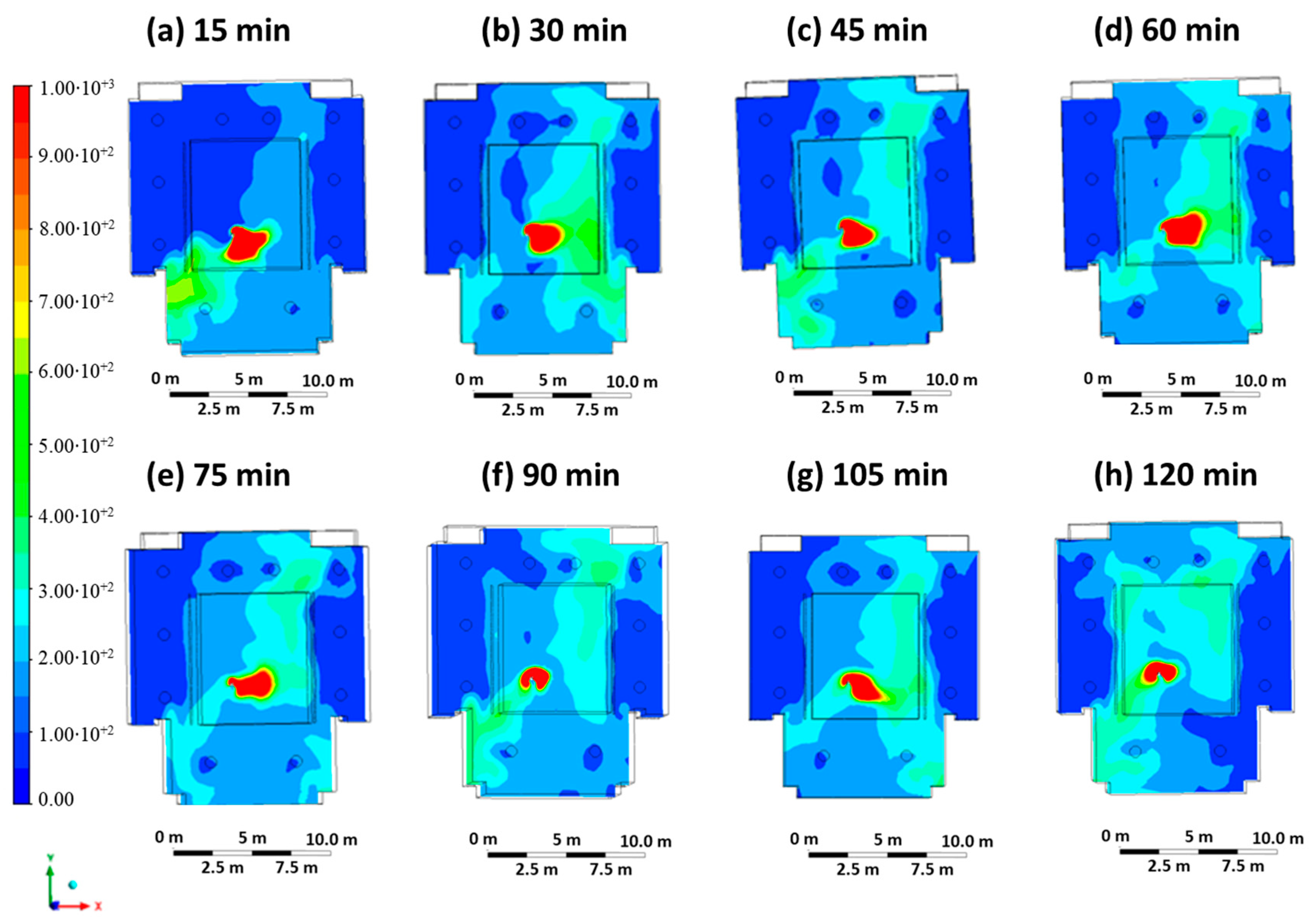
Case 1 represents the scenario in which the infected student does not wear the FFP2 mask and contaminates the other students and/or teachers present through the breathing process (entry velocity mouth equal to 1 m/s, entry velocity air equal to 0.3 m/s).
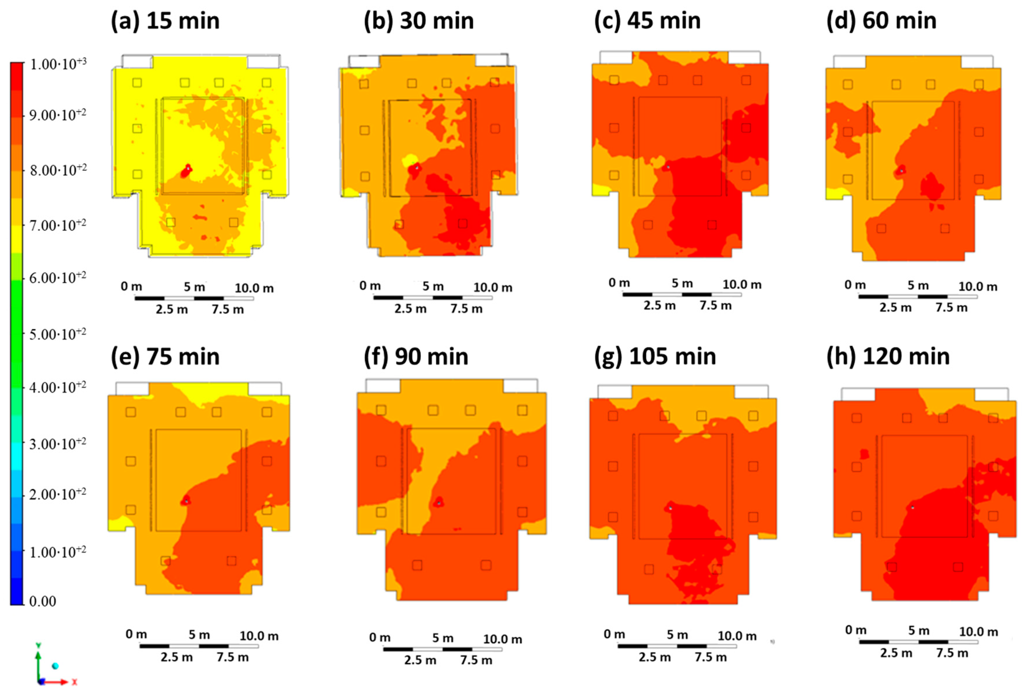
Figure 3 shows the contour plots of the CO2 concentration at intervals of 15 min, starting at time 0 (beginning of the lesson) up to 120 min (end of the lesson) on the sectional plane at a height of 1.65 m above the floor. The CO2 concentration, which is representative of the virus concentration, varies from 0 ppm (blue color) to 1000 ppm (red color), the minimum value. The highest levels of carbon dioxide concentrations are measured near the infected person and at the back of the classroom.
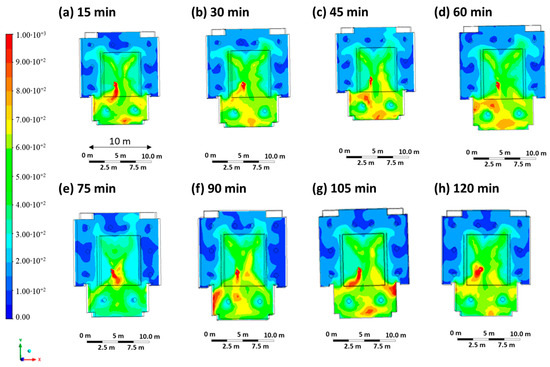
Figure 3.
Contour maps in terms of carbon dioxide concentration were obtained every 15 min in Case 1.
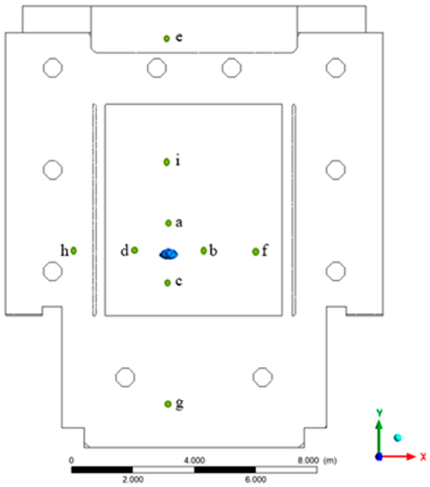
To compare the probability of infection, nine critical positions were defined (Figure 4). These points were used for a punctual evaluation of the infection risk as reported in Table 3 and were chosen at a different distance and direction with respect to the infester student in order to highlight the effect of the different investigated cases. Positions a, b, c, d were all one meter away from the infected person; positions i, f, h were 3 m away; position e (distance 7 m) represents the area where the teacher was normally located; position g (distance 5 m) represents another area s further away near the cloakroom and where students may be present.
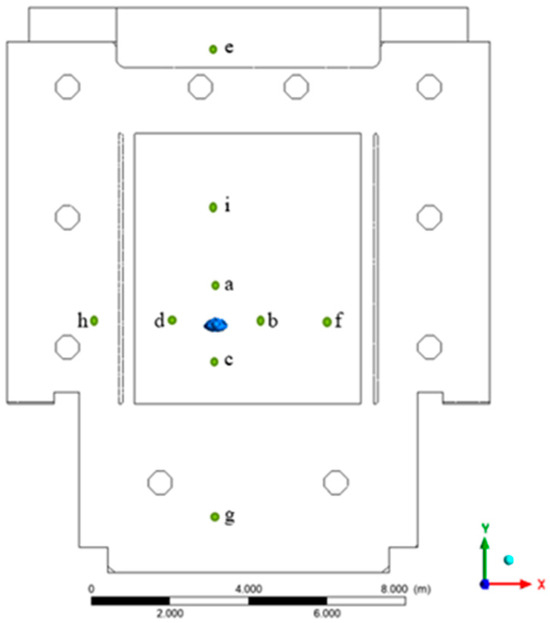
Figure 4.
Cut points used in the geometry for the evaluation of the infection risk.
Table 3.
Probability calculations were performed for Case 1 after 15 min, considering students and the teacher without DPI, with surgical and FFP2 masks.
Table 3 shows the probability values calculated after 15 min, assuming that the exposed student and/or teacher is not wearing PPE, is wearing a surgical mask or is wearing an FFP2 mask. The results at different times are reported in the Supplementary Materials (Tables S1–S3). At a time of 15 min (minimum exposure time), the minimum probability of infection is found at position e (the location where a potential teacher is present). It is equal to 0.6% if the exposed person is not wearing PPE, 0.4% if is wearing the surgical mask and 0.2% if is wearing the FFP2 mask. The most critical position is position c, where the probability of infection is 11.2% if no PPE is worn, while it drops to 8.0% if the surgical mask is worn and finally to 2.9% if the FFP2 mask is worn. The results at maximum exposure time (120 min, Table S3) show that the lowest values for the probability of infection are always associated with position e. The critical positions are position a and position b. The critical positions are positions a, b and c (distance of one meter from the infected person). It is important to point out that the results reflect the importance of maintaining a minimum safety distance of one meter, but that high infection probabilities can also occur at greater distances. The minimum distance to be maintained appears to be a function of the fluid dynamic conditions in the environment; the FFP2 mask, on the other hand, appears to be a highly effective tool that (when worn correctly) can significantly reduce the likelihood of infection (up to 75% less than without PPE).
3.2. Results Case 2
Case 2 is representative of an extremely critical scenario in which the infected person is not wearing a mask, and the ventilation system in the classroom is switched off (entry velocity mouth equal to 1 m/s, entry velocity air equal to 0 m/s). All small air changes through doors and/or windows were neglected in the simulations. Figure 5 shows the contour plots of the CO2 concentration at regular intervals of 15 min. A wave of CO2 concentration can be observed spreading through the classroom and reaching an almost uniform concentration after 2 h. As can be seen, high CO2 levels of up to 1000 ppm can be seen, particularly at the back of the classroom. It should be noted that the ventilation systems are all located on the ceiling, while the outlet areas are mainly located at the back of the classroom, so the cloud is preferentially located at the back due to the resulting flow field.

Figure 5.
Contour maps in terms of carbon dioxide concentration obtained every 15 min in Case 2.
Table 4 shows the results of the probability calculation after 15 min, assuming that the exposed potential student and/or teacher is not wearing PPE, is wearing a surgical mask or is wearing an FFP2 mask. Results are also reported for different timings (Tables S4–S6). Based on the minimum exposure time (15 min), it can be seen that the minimum value of the probability of infection occurs at positions e, h, d, f and is the same: 9.5% (no PPE), 6.8% (surgical mask), and 2.5% (FFP2 mask). The highest value for the probability of infection is found at positions a, b, c: 11.8% (no PPE), 8.4% (surgical mask), and 3.1% (FFP2 mask). An extremely critical scenario occurs at the maximum exposure time (120 min, Table S6): high infection probability values were achieved at all positions, varying in the range of 99.75–99.85% (no PPE). Wearing the FFP2 mask led to a 20% reduction in the probability of infection: the probability of infection varied between 77.69% and 80.31%. These results reflect the importance of ventilation: the values determined for the probability of infection are unacceptable, meaning that a university lecture is not possible without a ventilation system. With regard to the minimum distance to be maintained for social distancing (one meter), it can be seen that the virus spreads throughout the classroom with increasing exposure time and reaches all positions.
Table 4.
Probability calculations were performed for Case 2 after 15 min, considering students and the teacher without DPI, with surgical masks and with FFP2 masks.
3.3. Results Case 3
Case 3 represents a scenario in which the infected student wears an FFP2 mask and infects the other students and/or teachers present via the respiratory mechanism through air transmission (entry velocity mouth equal to 0.5 m/s, entry velocity air equal to 0.3 m/s). The ventilation system is in operation in its standard state in accordance with the COVID-19 regulations in force at the university. Figure 6 shows the contour plots of CO2 concentration at regular intervals of 15 min. The concentration map is similar to that of Case 1, but the areas of high concentration are more limited due to the infected person’s face mask.

Figure 6.
Contour maps in terms of carbon dioxide concentration obtained every 15 min in Case 3.
Table 5 shows the results of the probability calculation after 15 min, assuming that the exposed potential student and/or teacher is not wearing PPE, is wearing a surgical mask, or is wearing an FFP2 mask. Results are also reported for different timings (Tables S7–S9).
Table 5.
Probability calculations were performed for Case 3 after 15 min, considering students and the teacher without DPI, with surgical masks and with FFP2 masks.
Based on the minimum exposure time (15 min), the minimum values for the probability of infection at positions e, h, i are 0.6% (no PPE), 0.4% (surgical mask), and 0.2% (FFP2 mask). The highest values are found at positions a, b, c (distance of one meter from the infected person): 11.2% (no PPE), 8.0% (surgical mask), and 2.9% (FFP2 mask). Maintaining the minimum safety distance set at this exposure time allows a maximum percentage reduction in the probability of infection of 94%. At the maximum exposure time (120 min, Table S9), the minimum values for the probability of infection are at position e: 4.9% (no PPE), 3.4% (surgical mask), and 1.2% (FFP2 mask). This position is characteristic of the area near the blackboard where a potential teacher is present. The highest values for the probability of infection are found at positions a, b, c: 61.3% (no PPE), 48.6% (surgical mask), and 21.1% (FFP2 mask). The following probability values result at positions f and g: 50.3% (no PPE), 38.7% (surgical mask), and 16.1% (FFP2 mask). With increasing exposure time, the minimum safety distance of one meter appears to be insufficient, as even at distances of 3 or 5 m from the person, the values for the probability of infection are close to the values for positions a, b, c. Here, too, the minimum safety distance appears to depend on the ventilation conditions. The ventilation system plays a key role in preventing and controlling the spread of the virus. With position a, the FFP2 mask and an exposure time of 120 min (Table S9), a percentage decrease of 74% is observed compared to Case 2 (ventilation system switched off). Ventilation promotes the dilution of the virus in the room and thus reduces the probability of infection with SARS-CoV-2.
3.4. Results Case 4
Case 4 represents a scenario in which the infected student breathes without the FFP2 mask, and the ventilation system is characterized by a threefold increase in the inlet ventilation rate (inlet mouth velocity equal to 1 m/s, inlet air velocity equal to 0.9 m/s). Figure 7 shows the contour plots of CO2 concentration at regular intervals of 15 min, starting at time 0 (beginning of the hour) up to a maximum of 120 min (end of the hour). In comparison to Case 1, although the infected person is not wearing a mask, the high concentration zone is only maintained in the areas immediately next to the person due to the optimized ventilation.
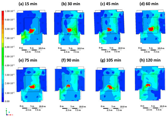
Figure 7.
Contour maps in terms of carbon dioxide concentration obtained every 15 min in Case 4.
Table 6 shows the results of the probability calculation after 15 min, assuming that the exposed potential student and/or teacher is not wearing PPE, is wearing a surgical mask or is wearing an FFP2 mask. Results are also reported for different timings (Tables S10–S12).
Table 6.
Probability calculations performed for Case 4 after 15 min, considering students and the teacher without DPI, with surgical masks and with FFP2 masks.
For the minimum exposure time (15 min), the lowest values for the probability of infection are at positions e, h, i: 0.6% (no PPE), 0.4% (surgical mask), and 0.2% (FFP2 mask). The maximum values are at positions a, b, c: 11.2% (no PPE), 8.0% (surgical mask), and 2.9% (FFP2 mask). For the maximum exposure time (120 min, Table S12), the lowest values for the probability of infection were at position h: 13.9% (no PPE), 3.4% (surgical mask), and 1.2% (FFP2 mask). The highest probability of infection was at positions d, b, c: 61.3% (no PPE), 48.6% (surgical mask), and 21.1% (FFP2 mask). The highest values for the probability of infection are found at positions d, b, c: 61.3% (no PPE), 48.6% (surgical mask), and 21.1% (FFP2 mask). At position g (5 m away from the infected person), the values for the probability of infection are lower than in the previously analyzed case studies: 18.1% (no PPE), 13.1% (surgical mask), and 4.9% (FFP2 mask). By increasing the ventilation flow rate, the area of influence of the virus can be limited to an area close to the infected student. If the speed of the airflow from the supply elements is greater, the virus can be transported out of the classroom more effectively and in less time. It is important to note that this effect is not consistent near the infected student as the student is modeled as a continuous virus source.
3.5. Results Case 5
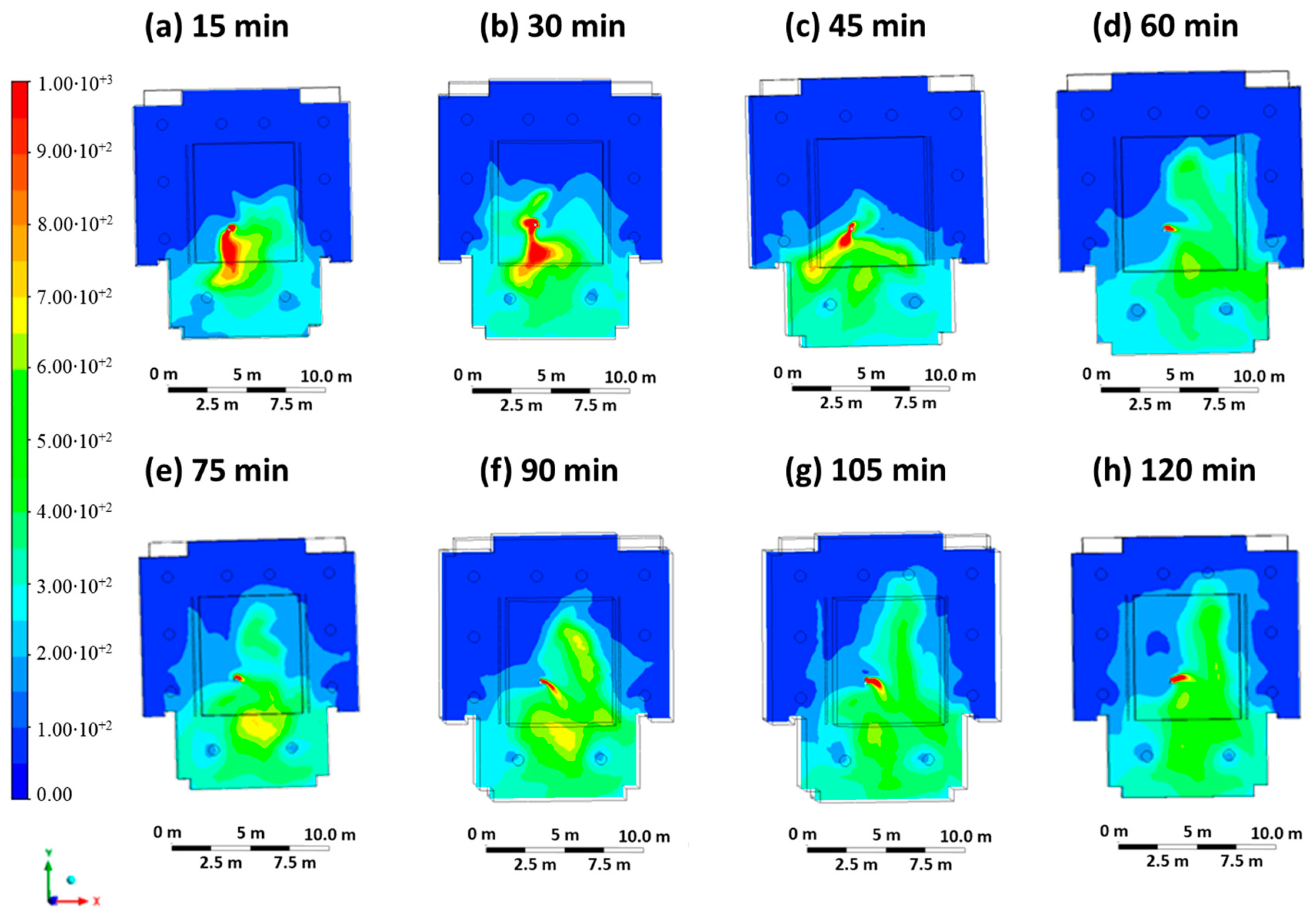
Case 5 represents a scenario in which the infected student is breathing wearing the FFP2 mask, and the ventilation system is characterized by a threefold increase in ventilation flow (inlet mouth velocity equal to 0.5 m/s, inlet air velocity equal to 0.9 m/s). Figure 8 shows the contour plots of the CO2 concentration at regular intervals of 15 min. Compared to Case 4, the presence of PPE in the infected person leads to a significant reduction in the extent of the high CO2 concentration zone, reaching an average concentration of less than 100 ppm in the classroom. In addition, the zone of high CO2 concentration is practically limited to the position of the infected student, which is an indication that a lower escape velocity combined with the presence of PPE and optimized ventilation can reduce the impact zone and, thus, the risk of infection.
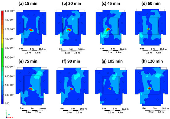
Figure 8.
Contour maps in terms of carbon dioxide concentration obtained every 15 min in Case 5.
Table 7 shows the results of the probability calculation after 15 min, assuming that the exposed potential student and/or teacher is not wearing PPE, is wearing a surgical mask or is wearing an FFP2 mask. Results are also reported for different timings (Tables S13–S15).
Table 7.
Probability calculations performed for Case 5 after 15 min, considering students and the teacher without DPI, with surgical masks and with FFP2 masks.
For the minimum exposure time (15 min), the minimum values for the probability of infection are at positions e, h, d, i, g: 0.6% (no PPE), 0.4% (surgical mask), 0.2% (FFP2 mask). Compared to the previous case studies, there are more positions characterized by a minimum value of the probability of infection; this results from the synergistic effect of ventilation (promotes the dilution of the virus in the classroom) and the FFP2 mask worn by the infected student, which reduces the momentum of the virus. The maximum values of the probability of infection are at positions a, b: 11.2% (no PPE), 8.0% (surgical mask), and 2.9% (FFP2 mask). For the maximum exposure time (120 min, Table S15), the lowest values for the probability of infection are at positions e, h, g: 4.9% (no PPE), 3.4% (surgical mask), and 1.2% (FFP2 mask). Here, too, there is a larger number of positions that are characterized by a minimum probability value. The maximum values for the probability of infection are at positions a, b: 61.3% (no PPE), 48.6% (surgical mask), and 21.1% (FFP2 mask). Overall, ventilation with tripled airflow does not reduce the maximum probability of infection values (the same maximum values analyzed in the previous cases are present), but it reduces and narrows the areas of maximum probability of infection by promoting and accelerating the dilution of the virus. Compared to Case 4, the situation improves in that the virus, which is characterized by a lower speed, reaches the same distances in a longer time so that the local virus concentration is definitely lower for the same exposure time and location. In addition, the return elements of the ventilation system are better able to remove the viruses so that the virus concentration in the classroom decreases.
4. Discussion
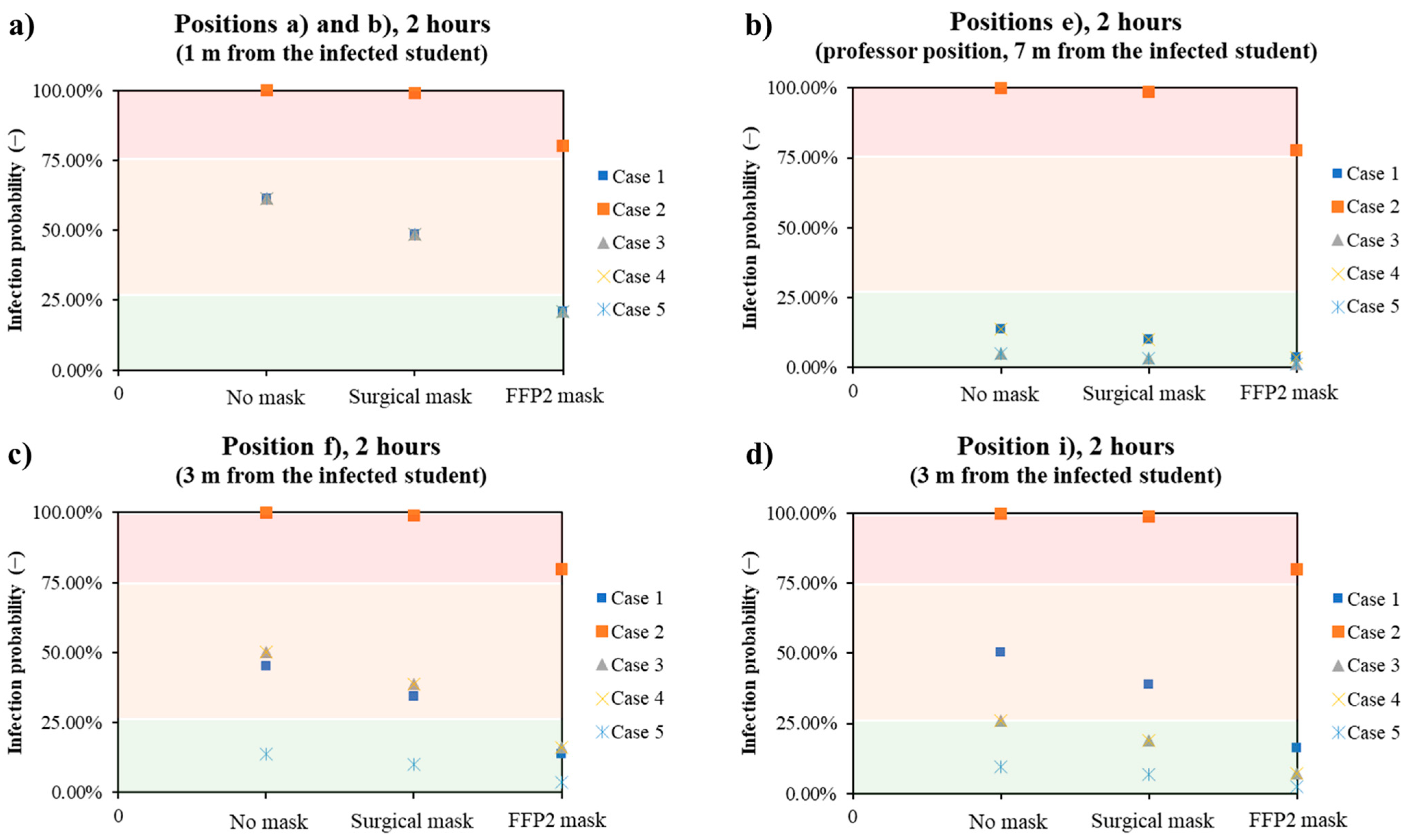
The results obtained are summarized in Figure 9. It can be seen that in the case of close distance (e.g., positions a and b at a distance of one meter from the infected student, Figure 9a), the use of FFP2 masks by those present in the classroom had the greatest effect. With the exception of Case 2, in which the probability of infection is greatest if the infected student is not wearing PPE and there is no ventilation, all other cases are comparable. The risk of infection only falls below 25% if the people present in the classroom wear the FFP2 mask, regardless of how well the room is ventilated and whether the infected student is wearing PPE. In the typical position that a professor assumes during a lecture (position e, Figure 9b), the probability of infection is always low, with the exception of Case 2. The maximum probability of infection is 13.9%, since neither the infected student nor all exposed persons wear a mask, while the minimum probability of infection is 1.2% if the exposed people wear an FFP2 mask, the infected student wears a mask and is ventilated normally/three times. At medium distances (e.g., 3 m, positions i and f), the values of the probability of infection depend strongly on the direction. At position i (Figure 9d), 3 m in front of the infected student, the probability of infection is always less than 25%, except in Case 2 and in the case of the infected student without a mask and the exposed people without or with a surgical mask. Triple ventilation had a significant impact on reducing the probability, as the comparison of the values for Case 3 and Case 5 shows. In the case of position f (Figure 9c), the presence of PPE has the greatest influence, as the probability of infection is comparable for single or triple ventilation.
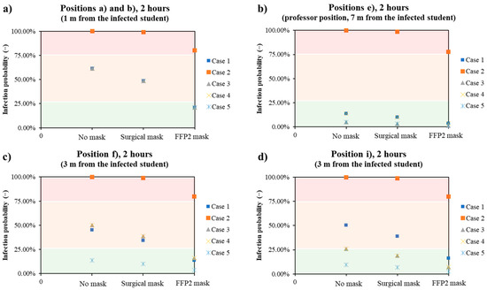
Figure 9.
Trends of the infection probability in the classroom as a function of the presence of DPI and kind in all the five analyzed cases for different positions: 1 m away from the infected student (a), typical professor position (7 m, (b)), and 3 m away from the infected student (c,d).
5. Conclusions
The design of ventilation and air conditioning systems in university halls and all busy enclosed spaces is of paramount importance to ensure the lowest possible likelihood of infection in the event of contamination by airborne pathogens. With the spread of the COVID-19 virus, this need has become even more important, and many ventilation systems have been suitably modified and/or reinforced to allow large numbers of people to stay for extended periods of time at low risk. This work simulated the ventilation system performance in classroom C of the Piazzale Tecchio complex of the University of Naples Federico II. The results highlight the crucial role of the combined ventilation and personal protective systems. After 60 min, the probability of infection at a distance of one meter from the infected person is 31% when the system is switched on and increases to 85% when the ventilation system is switched off. The system was then optimized by increasing the ventilation flow rate, which resulted in a probability of 14% with the same specifications. Finally, the importance of PPE, such as surgical and FFP2 masks, was analyzed, obtaining the following final probabilities for the previously analyzed case: 6.8% and 2.5%. The aim of this work was, of course, to demonstrate the possibility of applying normal risk analysis procedures for chemical processes to various problems using CFD simulations. In the future, we plan to perform CFD simulations on different setups and possibly try to formulate a more general theory developed using CFD results to provide specific guidance on risk mitigation.
Supplementary Materials
The following supporting information can be downloaded at: https://www.mdpi.com/article/10.3390/chemengineering8020037/s1, Figure S1: Graphical representation made with Ansys 2021R2 of the cut line positioned at the height of the breathing plane of the infected individual; Figure S2: Graphical representation made with Ansys 2021R2 of the cut line positioned at the height of the breathing plane of the infected individual; Table S1: Probability calculation performed for Case 1 at an interval of 30 min in the absence of PPE, in the presence of a surgical mask, in the presence of an FFP2 mask; Table S2: Probability calculation performed for Case 1 at an interval of 1 h in the absence of PPE, in the presence of a surgical mask, in the presence of an FFP2 mask; Table S3: Probability calculation performed for Case 1 at an interval of 2 h in the absence of PPE, in the presence of a surgical mask, in the presence of an FFP2 mask; Table S4: Probability calculation performed for Case 2 at an interval of 30 min in the absence of PPE, in the presence of a surgical mask, in the presence of an FFP2 mask; Table S5: Probability calculation performed for Case 2 at an interval of 1 h in the absence of PPE, in the presence of a surgical mask, in the presence of an FFP2 mask; Table S6: Probability calculation performed for Case 2 at an interval of 2 h in the absence of PPE, in the presence of a surgical mask, in the presence of an FFP2 mask; Table S7: Probability calculation performed for Case 3 at an interval of 30 min in the absence of PPE, in the presence of a surgical mask, in the presence of an FFP2 mask; Table S8: Probability calculation performed for Case 3 at an interval of 1 h in the absence of PPE, in the presence of a surgical mask, in the presence of an FFP2 mask; Table S9: Probability calculation performed for Case 3 at an interval of 2 h in the absence of PPE, in the presence of a surgical mask, in the presence of an FFP2 mask; Table S10: Probability calculation performed for Case 4 at an interval of 30 min in the absence of PPE, in the presence of a surgical mask, in the presence of an FFP2 mask; Table S11: Probability calculation performed for Case 4 at an interval of 1 h in the absence of PPE, in the presence of a surgical mask, in the presence of an FFP2 mask; Table S12: Probability calculation performed for Case 4 at an interval of 2 h in the absence of PPE, in the presence of a surgical mask, in the presence of an FFP2 mask; Table S13: Probability calculation performed for Case 5 at an interval of 30 min in the absence of PPE, in the presence of a surgical mask, in the presence of an FFP2 mask; Table S14: Probability calculation performed for Case 5 at an interval of 1 h in the absence of PPE, in the presence of a surgical mask, in the presence of an FFP2 mask; Table S15: Probability calculation performed for Case 5 at an interval of 2 h in the absence of PPE, in the presence of a surgical mask, in the presence of an FFP2 mask.
Author Contributions
Conceptualization, M.P. and A.D.B.; methodology, M.P., S.S. and A.D.B.; software, A.D.B.; validation, M.P. and A.D.B.; formal analysis, M.P. and A.D.B.; investigation, M.P. and S.S.; resources, A.D.B.; data curation, M.P. and S.S.; writing—original draft preparation, M.P.; writing—review and editing, A.D.B.; supervision, A.D.B.; project administration, A.D.B. All authors have read and agreed to the published version of the manuscript.
Funding
This research received no external funding.
Data Availability Statement
No new data were created or analyzed in this study. Data sharing is not applicable to this article.
Conflicts of Interest
The authors declare no conflicts of interest.
References
- Yin, P.; Brauer, M.; Cohen, A.J.; Wang, H.; Li, J.; Burnett, R.T.; Stanaway, J.D.; Causey, K.; Larson, S.; Godwin, W.; et al. The Effect of Air Pollution on Deaths, Disease Burden, and Life Expectancy across China and Its Provinces, 1990–2017: An Analysis for the Global Burden of Disease Study 2017. Lancet Planet. Health 2020, 4, e386–e398. [Google Scholar] [CrossRef] [PubMed]
- Zheng, W.; Hu, J.; Wang, Z.; Li, J.; Fu, Z.; Li, H.; Jurasz, J.; Chou, S.K.; Yan, J. COVID-19 Impact on Operation and Energy Consumption of Heating, Ventilation and Air-Conditioning (HVAC) Systems. Adv. Appl. Energy 2021, 3, 100040. [Google Scholar] [CrossRef]
- Guo, M.; Xu, P.; Xiao, T.; He, R.; Dai, M.; Miller, S.L. Review and Comparison of HVAC Operation Guidelines in Different Countries during the COVID-19 Pandemic. Build. Environ. 2021, 187, 107368. [Google Scholar] [CrossRef] [PubMed]
- Nazaroff, W.W. Indoor Bioaerosol Dynamics. Indoor Air 2016, 26, 61–78. [Google Scholar] [CrossRef]
- Portarapillo, M.; Di Benedetto, A. Methodology for Risk Assessment of COVID-19 Pandemic Propagation. J. Loss Prev. Process Ind. 2021, 72, 104584. [Google Scholar] [CrossRef] [PubMed]
- Kolmogorov, A. The Local Structure of Turbulence in Incompressible Viscous Fluid for Very Large Reynolds’ Numbers. Dokl. Akad. Nauk SSSR 1941, 30, 301–305. [Google Scholar]
- Bivolarova, M.; Ondráček, J.; Melikov, A.; Ždímal, V. A Comparison between Tracer Gas and Aerosol Particles Distribution Indoors: The Impact of Ventilation Rate, Interaction of Airflows, and Presence of Objects. Indoor Air 2017, 27, 1201–1212. [Google Scholar] [CrossRef]
- Zhang, Z.; Chen, X.; Mazumdar, S.; Zhang, T.; Chen, Q. Experimental and Numerical Investigation of Airflow and Contaminant Transport in an Airliner Cabin Mockup. Build. Environ. 2009, 44, 85–94. [Google Scholar] [CrossRef]
- Noakes, C.; Fletcher, L.; Sleigh, P. Comparison of Tracer Techniques for Evaluating the Behavior of Bioaerosols in Hospital Isolation Rooms. In Proceedings of the Healthy Buildings, Syracuse, NY, USA, 13–17 September 2009. [Google Scholar]
- Gao, N.P.; Niu, J.L.; Perino, M.; Heiselberg, P. The Airborne Transmission of Infection between Flats in High-Rise Residential Buildings: Particle Simulation. Build. Environ. 2009, 44, 402–410. [Google Scholar] [CrossRef]
- Xiaoping, L.; Jianlei, N.; Naiping, G. Spatial Distribution of Human Respiratory Droplet Residuals and Exposure Risk for the Co-Occupant under Different Ventilation Methods. HVAC R Res. 2011, 17, 432–445. [Google Scholar] [CrossRef]
- Beato-Arribas, B.; McDonagh, A.; Noakes, C.; Sleigh, P. Assessing the Near-Patient Infection Risk in Isolation Rooms. In Proceedings of the Healthy Buildings, Eindhoven, The Netherlands, 18–20 May 2015. [Google Scholar]
- Tretiakow, D.; Tesch, K.; Skorek, A. Mitigation Effect of Face Shield to Reduce SARS-CoV-2 Airborne Transmission Risk: Preliminary Simulations Based on Computed Tomography. Environ. Res. 2021, 198, 111229. [Google Scholar] [CrossRef]
- Suen, C.Y.; Kwok, H.H.L.; Tsui, Y.H.; Lui, K.H.; Leung, H.H.; Lam, K.W.; Hung, K.P.S.; Kwan, J.K.C.; Ho, K.F. Experimental and Computational Analysis of Surgical Mask Effectiveness Against COVID-19 in Indoor Environment. Aerosol Air Qual. Res. 2023, 23, 1–15. [Google Scholar] [CrossRef]
- Mirzaie, M.; Lakzian, E.; Khan, A.; Warkiani, M.E.; Mahian, O.; Ahmadi, G. COVID-19 Spread in a Classroom Equipped with Partition—A CFD Approach. J. Hazard. Mater. 2021, 420, 126587. [Google Scholar] [CrossRef] [PubMed]
- Rencken, G.K.; Rutherford, E.K.; Ghanta, N.; Kongoletos, J.; Glicksman, L. Patterns of SARS-CoV-2 Aerosol Spread in Typical Classrooms. Build. Environ. 2021, 204, 108167. [Google Scholar] [CrossRef]
- Burgmann, S.; Janoske, U. Transmission and Reduction of Aerosols in Classrooms Using Air Purifier Systems. Phys. Fluids 2021, 33, 033321. [Google Scholar] [CrossRef] [PubMed]
- He, R.; Liu, W.; Elson, J.; Vogt, R.; Maranville, C.; Hong, J. Airborne Transmission of COVID-19 and Mitigation Using Box Fan Air Cleaners in a Poorly Ventilated Classroom. Phys. Fluids 2021, 33, 033321. [Google Scholar] [CrossRef] [PubMed]
- Liu, S.; Deng, Z. Transmission and Infection Risk of COVID-19 When People Coughing in an Elevator. Build. Environ. 2023, 238, 110343. [Google Scholar] [CrossRef] [PubMed]
- Wang, F.; Zhang, T.; You, R.; Chen, Q. Evaluation of Infection Probability of COVID-19 in Different Types of Airliner Cabins. Build. Environ. 2023, 234, 110159. [Google Scholar] [CrossRef]
- Zhao, X.; Liu, S.; Yin, Y.; Zhang, T.; Chen, Q. Airborne Transmission of COVID-19 Virus in Enclosed Spaces: An Overview of Research Methods. Indoor Air 2022, 32, e13056. [Google Scholar] [CrossRef]
- Liu, M.; Liu, J.; Cao, Q.; Li, X.; Liu, S.; Ji, S.; Lin, C.H.; Wei, D.; Shen, X.; Long, Z.; et al. Evaluation of Different Air Distribution Systems in a Commercial Airliner Cabin in Terms of Comfort and COVID-19 Infection Risk. Build. Environ. 2022, 208, 108590. [Google Scholar] [CrossRef]
- Ripartizione Prevenzione e Protezione Attuazione Delle Misure per La Tutela Della Salute e Sicurezza per Lo Svolgimento Di Esami Di Profitto e Sedute Di Laurea in Presenza. Available online: https://www.unina.it/documents/11958/22035952/pg.2020.056683.pdf (accessed on 2 January 2023).
- Shao, X.; Li, X. COVID-19 Transmission in the First Presidential Debate in 2020. Phys. Fluids 2020, 32, 115125. [Google Scholar] [CrossRef] [PubMed]
- Wells, W.F. Airborne Contagion and Air Hygiene. JAMA 1955, 159, 90. [Google Scholar]
- Riley, C.E.; Murphy, G.; Riley, R.L. Airborne Spread of Measles in a Suburban Elementary School. Am. J. Epidemiol. 1978, 107, 421–432. [Google Scholar] [CrossRef] [PubMed]
- Dai, H.; Zhao, B. Association of the Infection Probability of COVID-19 with Ventilation Rates in Confined Spaces. Build. Simul. 2020, 13, 1321–1327. [Google Scholar] [CrossRef] [PubMed]


Disclaimer/Publisher’s Note: The statements, opinions and data contained in all publications are solely those of the individual author(s) and contributor(s) and not of MDPI and/or the editor(s). MDPI and/or the editor(s) disclaim responsibility for any injury to people or property resulting from any ideas, methods, instructions or products referred to in the content. |
© 2024 by the authors. Licensee MDPI, Basel, Switzerland. This article is an open access article distributed under the terms and conditions of the Creative Commons Attribution (CC BY) license (https://creativecommons.org/licenses/by/4.0/).