Closed-Loop Stability of a Non-Minimum Phase Quadruple Tank System Using a Nonlinear Model Predictive Controller with EKF

Abstract

The dynamics of a quadruple tank system (QTS) represent an extensive class of multivariate nonlinear uncertain systems found in the industry. It has been established that changes in split fractions affect the transmission zero location, thereby altering the operating conditions between the minimum and non-minimum phase regions. The latter is difficult to control as more fluid flows into the two upper tanks than into the two bottom tanks, resulting in competing effects between the initial and final system responses. This attribute, alongside nonlinearity, uncertainties, constraints, and a multivariate nature, can degrade closed-loop system performance, leading to instability. In this study, we addressed the aforementioned challenges by designing controllers for the regulation of the water flow in the two bottom tanks of the QTS. For comparative analysis, three controller algorithms—a nonlinear model predictive controller (NMPC), NMPC augmented with an extended Kalman filter (i.e., NMPC-EKF) and linear model predictive controller (LMPC)—were considered in the analysis and design of the control mechanism for the quadruple water level system in a non-minimum phase condition via the Matrix Laboratory (MATLAB) simulation package environment. The simulated and real-time results in the closed loop were analyzed, and the controller performances were considered based on faster setpoint responses, less oscillation, settling time, overshoot, and smaller integral absolute error (IAE) and integral square error (ISE) under various operational conditions. The study showed that the NMPC, when augmented with an EKF, is effective for the control of a QTS in the non-minimum phase and could be designed for more complex, nonlinear, and multivariable dynamics systems, even in the presence of constraints.

1. Introduction

Problems are frequently encountered in process industries (such as oil and gas, wastewater treatment, power plants, pharmaceutical, and food industries). Level control in tanks and other process equipment is critical and is of great interest to systems engineers because inadequate level control can result in system shutdown, waste of power, process vessel overflow or emptying, unsafe working conditions, shorter life span of equipment, etc.

This study focuses on the practical application of NMPCs to a real-time experimental four-tank control rig. The four-tank process was designed at Lund University to study multivariable systems with performance limitations by conditions that include right half-plane (RHP) zeros and model uncertainties [1]. A four-tank system, often called a quadruple tank system (QTS), exhibits transmission zero as it transitions from the minimum phase (MP) to the non-minimum phase (NMP) by simple valve adjustment. NMP systems are characterized by RHP zeros. Systems with an RHP of zero present difficulties when applying control strategies. Both NMP and unstable systems occur mostly in industrial processes. Therefore, systems engineers must be aware of this kind of process because they are important sources of control problems in real multivariable systems.

Generally, a control problem is formulated such that an NMPC is preferred as the appropriate choice of controller owing to its handling of the system’s input and output constraints, nonlinearity, multivariate interactions, and non-minimum phase characteristics. The NMPC problem is formulated similarly to the LMPC problem since it shares the majority of the LMPC’s fundamental characteristics [2]. However, NMPCs use nonlinear models for predictions rather than linear system models [3]. However, nonlinear models are attractive for the control of systems with substantial nonlinearities because they faithfully reproduce the behaviour of the managed system. In the presence of unforeseen disturbances and modifications to the desired state trajectory, the current state of a controlled system closely follows the ideal state trajectory. In other words, a suitable control action is performed to direct the state toward the reference trajectory if it is currently far from it. A suitable control action is made to regulate the state in the presence of disturbances [4] if the present state is already sufficiently near to the reference trajectory, making the control problem simple to solve. However, owing to nonlinearity and coupling effects, control problems can often be difficult to solve. When issues with static output feedback stabilization are taken into consideration, the influence of the non-minimum phase, which is defined by the presence of dead time and an unstable inverse, is not desired in control procedures [5]. The stability of a closed loop is not ensured by this feedback law [6]. NMPCs specifically make a stable system unstable [7]. This work proposed and implemented the augmentation of the EKF to the designed NMPC to estimate states and remove offsets from the outputs with the following objectives: (a) interface a quadruple tank system with a microcontroller board for a direct digital control (DDC); (b) design and implement an NMPC augmented with an extended Kalman filter (NMPC-EKF) and a linear model predictive controller (MPC) for the system; and (c) evaluate the performances of the designed controllers for non-minimum phase conditions.

2. Materials and Methods

2.1. Theoretical Framework

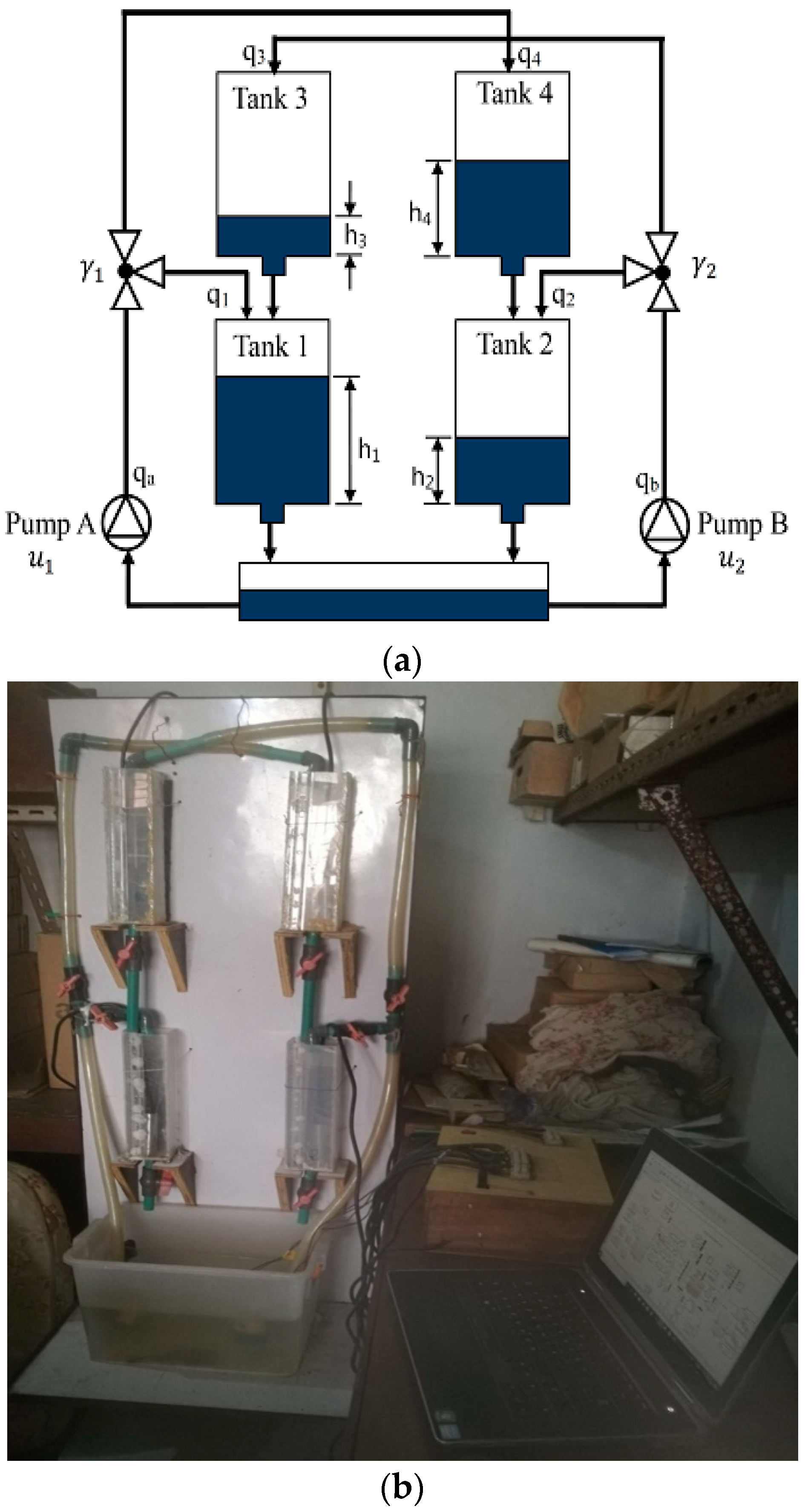
Consider the experimental setup of a quadruple tank system specifically designed and fabricated in our laboratory to investigate the control of a non-minimum phase system using the NMPC technique. The system consists of four interconnected water tanks and two pumps. The inputs were the voltages of the two pumps. The outputs were the water levels in the two lower tanks (h₁ and h₂). The setup, though very simple, can be used to illustrate interesting multivariable nonlinear phenomena. The positions of the valves are denoted as γ1 and γ2. Tank 3 and tank 4 were placed above tank 1 and tank 2 to drain water directly by the action of gravity. The flow from each of the pumps was split into two by using a three-way valve (flow splitter or flow divider). The output of pump 1 is split between tank 1 and tank 4, whereas that of pump 2 is also split between tank 2 and tank 3. As a result, the flow to each pump’s output tanks—a lower and an upper diagonal tank—is regulated by the valve position, shown by the symbol γ. At the bottom of each tank was a discharge valve that allowed liquid to flow into the tank beneath it. The reservoir tank at the bottom receives discharge from tanks 1 and 2. It is an MIMO system because of the interactions and strong connection between the tanks. Figure 1a depicts a schematic of the quadruple tank system.

2.2. Dynamic Model Development of the System

Theoretical mass balance using Bernoulli’s law was used to investigate and control the behavior of the process. Employing these laws using the flow rate data in

Table 1. Flow rates into the tanks by pumps.

Tank	Pump1	Pump2
1	$k_1{q}_1{\gamma }_1$	-
2	-	$k_2{q}_2{\gamma }_2$
3	-	$k_2{q}_2\left(1-{\gamma }_2\right)$
4	$k_1{q}_1(1-{\gamma }_1)$	-

, after simplification, the nonlinear dynamic models of the QTS are derived as

$$\dot{h_1}(t)=\frac{1}{A_1}(-a_1{\alpha }_1\sqrt{2g{h}_1}+a_3{\alpha }_3\sqrt{2g{h}_3}+k_1{q}_1{\gamma }_1)$$

(1)

$$\dot{h_2}(t)=\frac{1}{A_2}(-a_2{\alpha }_2\sqrt{2g{h}_2}+a_4{\alpha }_4\sqrt{2g{h}_4}+k_2{q}_2{\gamma }_2)$$

(2)

$$\dot{h_3}(t)=\frac{1}{A_3}(-a_3{\alpha }_3\sqrt{2g{h}_3}+k_2{q}_2(1-{\gamma }_2))$$

(3)

$$\dot{h_4}(t)=\frac{1}{A_3}(-a_4{\alpha }_4\sqrt{2g{h}_4}+k_1{q}_1(1-{\gamma }_1))$$

(4)

The parameters of the system are defined in the Appendix A.

2.3. Non-Minimum Phase Characteristics

A system that is causal and stable but whose inverse is causal and unstable is known as a non-minimum phase system. In a quadruple tank system, the non-minimum phase (NMP) occurs when the fraction of liquid entering the upper tanks is greater than that entering the lower tanks [8,9,10]. The valves were regulated to control the flow ratio to the maximum value for the two upper tanks. The flow ratio ($\gamma$) is obtained as a fraction by measuring the volumes of water in the two diagonal tanks of the respective pumps, and it obeys the phase configuration 0 < γ1 + γ2 < 1. This implies that the zeros of the corresponding transfer functions are in the right half-plane. When the system is run in the non-minimum phase, there is a pole shift to the right half of the s-plane. The study procedure is made unpredictable by this.

2.4. Control Algorithms

The two control algorithms follow the same path, except for the use of the linearized model of the plant by the LMPC and the solving of the nonlinear programming problem by the NMPC.

2.4.1. Linear Model Predictive Control (LMPC)

Equations (1)–(4) have square root terms that account for nonlinearity, which makes designing controllers more difficult. The linearized state-space model of the system is given as

$$\dot{\mathit{h}}=\mathit{A}\mathit{h}+\mathit{B}\mathit{q}$$

(5)

$$\mathit{y}=\mathit{C}\mathit{h}+\mathit{D}\mathit{q}$$

(6)

In order to obtain the transfer function of a non-linear model, linearization has to be carried out to obtain the state-space representation of the model. This follows the fact that the Laplace transform of a non-linear model cannot be obtained unless linearization has been carried out. With details of the procedure shown in the Appendix A, the state-space representation using Taylor’s series rule for linearization of the quadruple tank process is shown below:

$$\left[\begin{array}{c}\frac{d{h}_1}{dt}\\ \frac{d{h}_2}{dt}\\ \frac{d{h}_3}{dt}\\ \frac{d{h}_4}{dt}\end{array}\right]=\left[\begin{array}{cccc}-0.2829& 0& 1.2858& 0\\ 0& -0.1858& 0& 0.3269\\ 0& 0& -1.2858& 0\\ 0& 0& 0& -0.3269\end{array}\right]\left[\begin{array}{c}{h}_1\\ h_2\\ h_3\\ h_4\end{array}\right]+\left[\begin{array}{cc}0.01303& 0\\ 0& 0.005769\\ 0& 0.02214\\ 0.01395& 0\end{array}\right]\left[\begin{array}{c}{q}_1\\ q_2\end{array}\right]$$

(7)

$$y=\left[\begin{array}{cccc}1& 0& 0& 0\\ 0& 1& 0& 0\end{array}\right]\left[\begin{array}{c}{h}_1\\ h_2\\ h_3\\ h_4\end{array}\right]+\left[\begin{array}{cc}0& 0\end{array}\right]\left[\begin{array}{c}{q}_1\\ q_2\end{array}\right]$$

(8)

where y represents the desired output variables which, in this case, are tank 1 and tank 2 levels (h₁ and h₂); $q_{1}and{q}_2$ are the input variables representing pump 1 and pump 2, respectively.

The above state space was used to design the LMPC controller with a control horizon and prediction horizon (prediction of state performed over a finite future time interval) of 2 and 50, respectively.

2.4.2. Validation of Operating Phases

The NMP had at least one zero value in the RHP. The poles of the system are the eigenvalues of the matrix obtained, which were used for the stability analysis, and the eigenvalues for the phase indicated that the system was open-loop stable. However, the zeros of multivariable systems, such as the system under consideration, are hidden dynamics [1]. However, to establish this fact, a pole-zero map is required to confirm that the obtained multivariable transfer functions are truly representative of an NMP. For the operating non-minimum phase, the zeros of the system after linearization and computation of the system transfer function are (−2.2053, 0.5926), which implies that the three-way split valve was preset correctly.

2.4.3. Constrained NMPC Formulation

There are two important separate parts of the NMPC problem: a prediction model formulation and a solution to the optimal control problem. In order to anticipate the trajectory of the future state, the nominal model of the controlled system was iterated several times to create the prediction model.

Using the model Equations (1)–(4), a discrete-time nonlinear nominal state-space model in its general form is given by

$$x\left(k+1\right)=f\left(x\left(k\right),q\left(k\right)\right)$$

(9)

$$y\left(k\right)=g\left(x\left(k\right)\right)$$

(10)

2.4.4. State Prediction Model

By repeating the state transition equation provided by Equation (6), future states can be predicted. Here is a description of the state prediction model:

$$x\left(k+1\text{| }k\right)=f\left(x\left(k\text{| }k\right),q\left(k\text{| }k\right)\right)$$

(11)

$$x\left(k+2\text{| }k\right)=f\left(x\left(k+1\text{| }k\right),q\left(k+1\text{| }k\right)\right)$$

(12)

$$x\left(k+3\text{| }k\right)=f\left(x\left(k+2\text{| }k\right),q\left(k+2\text{| }k\right)\right)$$

(13)

$$x\left(k+N_c\text{| }k\right)=f\left(x\left(k+N_c-1\text{| }k\right),q\left(k+N_c-1\text{| }k\right)\right)$$

(14)

$$x\left(k+N_p\text{| }k\right)=f\left(x\left(k+N_p-1\text{| }k\right),q\left(k+N_c-1\text{| }k\right)\right)$$

(15)

where “ $\text{| }k$” means that at time instant k, the state is expected. Up until a certain number of time steps in the prediction horizon Np is reached, this pattern is followed. If N_c < N_p, the last set of control values $q\left(k+N_c-1\text{| }k\right)$ in the control sequence is maintained for the remaining (N_p–N_c) time steps, where, N_c is the control horizon. Note that in the formulation of the NMPC, N_c is always set to be either less than or equal to N_p. Equations (11)–(15) demonstrate this. The sequence of control inputs and the expected state trajectory can be represented in vector form as follows:

$$\mathit{X}\left(k\right)=\left[\begin{array}{c}x\left(k+1\text{| }k\right)\\ x\left(k+2\text{| }k\right)\\ x\left(k+3\text{| }k\right)\\ ⋮\\ x\left(k+N_p\text{| }k\right)\end{array}\right]$$

(16)

$$\mathit{Q}\left(k\right)=\left[\begin{array}{c}q\left(k\text{| }k\right)\\ q\left(k+1\text{| }k\right)\\ q\left(k+2\text{| }k\right)\\ q\left(k+3\text{| }k\right)\\ ⋮\\ q\left(k+N_p-1\text{| }k\right)\end{array}\right]$$

(17)

Using Equations (16) and (17), Equations (11)–(15) are summarized as a function of the current state $x\left(k\right)$= $x\left(k\text{| }k\right)$ and predicted control input vector $\mathit{Q}\left(k\right)$, as follows:

$$\mathit{X}\left(k+1\right)=f\left(x\left(k\right),\mathit{Q}\left(k\right)\right)$$

(18)

2.4.5. Output Prediction Model

The projected output estimates of the system are obtained by propagating the predicted state estimates provided by Equation (16) but derived by Equation (18) through the output equation provided by Equation (10). The following is a description of the output prediction model:

$$y\left(k+1\text{| }k\right)=g\left(x\left(k+1\text{| }k\right)\right)$$

(19)

$$y\left(k+2\text{| }k\right)=g\left(x\left(k+2\text{| }k\right)\right)$$

(20)

$$y\left(k+1\text{| }k\right)=g\left(x\left(k+1\text{| }k\right)\right)$$

(21)

$$y\left(k+N_p\text{| }k\right)=g\left(x\left(k+N_p\text{| }k\right)\right)$$

(22)

The following vector form can be used to represent the predicted output estimates:

$$\mathit{Y}\left(k\right)=\left[\begin{array}{c}y\left(k+1\text{| }k\right)\\ y\left(k+2\text{| }k\right)\\ y\left(k+3\text{| }k\right)\\ ⋮\\ y\left(k+N_p\text{| }k\right)\end{array}\right]$$

(23)

Equation (10) can be written in a compact form:

$$\mathit{Y}\left(k\right)=g\left(x\left(k\right)\right)$$

(24)

In essence, the NMPC method resolves an optimum control problem to identify the best order of control inputs so that the controlled system’s future outputs follow a specified output trajectory that is provided by

$${\mathit{Y}}^{\mathit{s}\mathit{p}}\left(k\right)=\left[\begin{array}{c}{y}^{sp}\left(k+1\text{| }k\right)\\ y^{sp}\left(k+2\text{| }k\right)\\ y^{sp}\left(k+3\text{| }k\right)\\ ⋮\\ y^{sp}\left(k+N_p\text{| }k\right)\end{array}\right]$$

(25)

$\mathit{Y}\left(k\right)$ and $\mathit{Q}\left(k\right)$ are the predicted output and control input trajectories that are generated by the NMPC algorithm at every time step k, while ${\mathit{Y}}^{sp}\left(k\right)$ is the desired output trajectory. At each time step, these are given into the NMPC algorithm to build a corresponding cost function that is a component of the optimal control problem.

2.4.6. Cost Function

There are three cost functions that make up the quadratic cost function: $J_y$, $J_q$, and $J_{dq}$. The cost function $J_y$ penalizes the deviation between the predicted output $\mathit{Y}\left(k\right)$ and the desired output trajectories ${\mathit{Y}}^{sp}\left(k\right)$. The quadratic form of $J_q$ is weighted with positive (semi-) definite weighing matrices $(W_y\left(k\right),\dots W_y(k+N_p-1))$ and thus $J_y$ is given by

$$J_y={\sum }_{i=0}^{N_p}{(y(k+i\text{| }k)-y^{sp}\left(k+i\text{| }k\right))}^T{W}_y\left(k+i\right)\left(y\left(k+i\text{| }k\right)-y^{sp}\left(k+i\text{| }k\right)\right)$$

(26)

When the matrices $(W_y\left(k\right),\dots W_y\left(k+N_p-1\right))$ are positioned along a positive (semi-definite) weighing matrix of the appropriate size’s main diagonal, $W_y\left(k\right)$ is

$$W_y\left(k\right)=\left[\begin{array}{cccc}{W}_y\left(k\right)& 0& \cdots & 0\\ 0& W_y\left(k+1\right)& \cdots & ⋮\\ ⋮& ⋮& \ddots & 0\\ 0& \cdots & 0& W_y\left(k+N_p-1\right)\end{array}\right]$$

(27)

Cost function $J_y$ in compact form is

$$J_y=Y\left(k\right)-Y^{sp}\left(k\right){)}^T{W}_y\left(k\right)\left(Y\left(k\right)-Y^{sp}\left(k\right)\right)$$

(28)

Cost function $J_q$ penalizes control input magnitudes in the control sequence $\mathit{Q}\left(k\right)$. The quadratic form of the $J_q$ is weighted with the positive (semi-) definite weighing matrices $(W_q\left(k\right),\dots W_q\left(k+N_p-1\right))$.

$$J_q={\sum }_{i=0}^{N_p-1}q{\left(k+i\text{| }k\right)}^T{W}_q\left(k+i\right)(q\left(k+i\text{| }k\right)$$

(29)

$$W_q\left(k\right)=\left[\begin{array}{cccc}{W}_q\left(k\right)& 0& \cdots & 0\\ 0& W_q\left(k+1\right)& \cdots & ⋮\\ ⋮& ⋮& \ddots & 0\\ 0& \cdots & 0& W_q\left(k+N_p-1\right)\end{array}\right]$$

(30)

$$J_q=Q{\left(k\right)}^T{W}_q\left(k\right)Q\left(k\right)$$

(31)

$J_{dq}$ is a cost function that penalizes input rate magnitudes. The quadratic form of the $J_{dq}$ is weighted with the positive (semi-) definite weighing matrices $(W_{dq}\left(k\right),\dots W_{dq}\left(k+N_p-1\right))$.

$$J_{dq}={\sum }_{i=0}^{N_p-1}dq{\left(k+i\text{| }k\right)}^T{W}_{dq}\left(k+i\right)(dq\left(k+i\text{| }k\right)$$

(32)

where

$$d{q}_i=q_i-q_{i-1}$$

(33)

Similarly,

$$J_{dq}=dQ{\left(k\right)}^T{W}_{dq}\left(k\right)dQ\left(k\right)$$

(34)

The total cost function is

$$J=J_y+J_q+J_{dq}$$

(35)

To analyze the difference in system performance and precision, the prediction horizon 𝑁_𝑝, is varied within a finite range of values. An infinitely long prediction horizon would be the ideal choice, which would provide perfect performance. However, practically, it is impossible to implement an infinitely long prediction horizon. It is desirable to use a large but finite horizon. In addition, the controller performance decreased when the control horizon was set to high values. It is worth noting, however, that choosing a long prediction horizon implies that more variables must be solved in the optimization problem. This makes solving the problem complex.

The prediction horizon $N_p$ was taken as 100, and the control horizon was taken to be 1. For the weighing matrices $W_y$ (weight on output) and $W_Q$ (weight on input), they were tuned until the desired performance was achieved. This is a trade-off between a smooth signal and fast system performance. If a smooth signal is desired, then the ratio of $W_y$ to $W_Q$ is to be low, and if one wants a fast system, then the ratio should be quite high. Since only tank 1 and tank 2 levels are being controlled, the matrix $W_y$ is chosen as a diagonal matrix with nonzero values on the positions that correspond to states 1 and 2 since tank 1 and tank 2 levels control is desired. $W_Q$ is a diagonal 2 × 2 matrix.

The constraints placed on the input and output are also important. As dictated by the pump specifications, the maximum input flow is 255 PWM. Therefore, the upper and lower limits, respectively, were 255 PWM ($q_{max}$) and 0 ($q_{min}$). The constraints applicable to the tank levels were associated with their heights. The lower and upper limits of the tank levels were 30 and 0 cm, respectively.

2.5. Optimal Control Problem (OCP)

In order to maximize the controlled system’s performance, J must be minimized with respect to U(k), while also taking the system’s equality and inequality restrictions into consideration. J can only ever have a minimum value of zero. The optimum control problem (OCP) for MPC is the formal name for this minimization problem. Depending on whether constrained fulfillment is sought, the OCP can be formulated as either an unconstrained or a constrained OCP. A constrained OCP was employed in this study to formulate the constrained NMPC controller. The capacity of NMPC schemes to address system limitations in their formulations makes them more desirable for the control of nonlinear dynamic systems. The OCP problem is posed as (when constraints are present):

$$\min U\left(x\right){(Y\left(k\right)-Y^{sp}\left(k\right))}^T{W}_y\left(k\right)\left(Y\left(k\right)-Y^{sp}\left(k\right)\right)+Q{\left(k\right)}^T{W}_q\left(k\right)Q\left(k\right)+dQ{\left(k\right)}^T{W}_{dq}\left(k\right)dQ\left(k\right)$$

(36)

subject to

$$x\left(k+i\text{| }k\right)=f\left(x\left(k+i-1\text{| }k\right),q\left(k+i-1\text{| }k\right)\right)$$

(37)

$$y\left(k+i\text{| }k\right)=g\left(x\left(k+i-1\text{| }k\right)\right),i=0,\dots ,N_p-1$$

(38)

$$q\left(k+i\text{| }k\right)=q\left(k+N_c-1\text{| }k\right),i=N_c,\dots ,N_p-1$$

(39)

$$X_{min}\le X\left(k\right)\le X_{max}$$

(40)

$$Q_{min}\le Q\left(k\right)\le Q_{max}$$

(41)

$$Y_{min}\le Y\left(k\right)\le Y_{max}$$

(42)

$$d{Q}_{min}\le dQ\left(k\right)\le d{Q}_{max}$$

(43)

where $X_{min}$, $Y_{min}$, $Q_{min}$, and $d{Q}_{min}$ are the lower bounds of the state trajectory, system output trajectory, sequence of control inputs, and input rate, respectively. $X_{max}$,$Y_{max}$, $Q_{max}$, and $d{Q}_{max}$ are the upper bounds of the state trajectory, system output trajectory, sequence of control inputs, and input rate, respectively. Equations (40)–(43) describe the inequality constraints of the system, and Equations (37)–(39) describe the equality constraints.

2.6. Discretization of OCP

This is a process of transforming OCP into standard nonlinear programming (NLP) to solve the OCP using solution techniques such as sequential quadratic programming (SQP).

A standard NLP is described as

$$\min F\left(z\left(k\right)\right)$$

subject to

$$H\left(z\left(k\right)\right)=0$$

(44)

$$G\left(z\left(k\right)\right)\le 0$$

(45)

where F is the cost function of the problem and $z\left(k\right)$ is the optimization variable.

2.6.1. Linear Approximation of Nonlinear State Estimation

The EKF approximates the Gaussian random variable (GRV) distribution of state. In the first-order linearization of the nonlinear dynamic system, the GRV was transformed analytically [11] at every instant. Because it is essential to consider the linearization of a nonlinear dynamic system, the manner in which the EKF performs the linearization is discussed. Consider the nonlinear general structure of the quadruple tank system with the disturbance additive defined by Equations (46)–(49).

$$\dot{h_1}\left(t\right)=\frac{1}{A_1}\left(-a_1{\alpha }_1\sqrt{2g{h}_1}+a_3{\alpha }_3\sqrt{2g{h}_3}+k_1{q}_1{\gamma }_1+d_1\right)$$

(46)

$$\dot{h_2}\left(t\right)=\frac{1}{A_2}\left(-a_2{\alpha }_2\sqrt{2g{h}_2}+a_4{\alpha }_4\sqrt{2g{h}_4}+k_2{q}_2{\gamma }_2+d_2\right)$$

(47)

$$\dot{h_3}\left(t\right)=\frac{1}{A_3}\left(-a_3{\alpha }_3\sqrt{2g{h}_3}+k_2{q}_2\left(1-{\gamma }_2\right)+d_3\right)$$

(48)

$$\dot{h_4}\left(t\right)=\frac{1}{A_3}\left(-a_4{\alpha }_4\sqrt{2g{h}_4}+k_1{q}_1\left(1-{\gamma }_1\right)+d_4\right)$$

(49)

Using Euler to discretize Equations (46)–(49), we obtained the equations in the Appendix A. It was determined that the functions $f$ were sufficiently differentiable and continuous in $x$ so that each one had a valid Taylor series expansion. The Jacobians process model was computed as described in the Appendix A.

2.6.2. EKF-Based NMPC Algorithm

EKF-based NMPC extended the performance of the standard NMPC controller to the rejection of disturbances and handling of mismatches from the plant to the model, which can be observed when modeling dynamic systems. The algorithm for the formulation of the EKF (augmented with NMPC) is presented below.

$$Initializationatk=0$$

$$Fork=1,\dots \infty ;$$

• Time-update equations:

  $$J_f={\nabla }_{x}f\left(x,q\left(k-1\right)\right)$$

  (50)

  $${\widehat{x}}^{-}\left(k\right)=f\left(\widehat{x}\left(k-1\right),q\left(k-1\right)\right)$$

  (51)

  $$P_x^{-}=\varnothing J_f{P}_x\left(k-1\right)J_f^T+R_w$$

  (52)
• Measurement-update equations:

  $$J_f={\nabla }_{x}h\left(x\right)$$

  (53)

  $$K\left(k\right)=P_x^{-}\left(k\right)J_h^T{\left[J_h{P}_x^{-}\left(k\right)J_h^T+R_v\right]}^{-1}$$

  (54)

  $${\widehat{y}}_k^{-}=h\left({\widehat{x}}^{-}\left(k\right)\right)$$

  (55)

  $$\widehat{x}\left(k\right)={\widehat{x}}^{-}\left(k\right)+K\left(k\right)\left[y\left(k\right)-{\widehat{y}}_k^{-}\right]$$

  (56)

  $$P_x=\left[I-K\left(k\right)J_h\right]P_x^{-}\left(k\right)$$

  (57)

  where

${\widehat{x}}^{-}\left(k\right)$ is the predicted estimates of the states,

$P_x^{-}\left(k\right)$ is the estimation error of the state covariance,

$K$ is Kalman gain,

$k$ is time instant,

$I$ is an identity matrix,

$\varnothing$ (phi) is a measure of how aggressively deviation in measurements affects state estimation,

and $R_{w}and{R}_v$ are the covariance matrices of the process noise and measurement noise, respectively.

The values of quadruple tank physical parameters are given in

Table A1. Model physical parameter and nominal operating points.

Parameters	Values	Units
$q_{1_0}$	$170$	${\mathrm{cm}}^3/\mathrm{s}$
$q_{2_0}$	$170$	${\mathrm{cm}}^3/\mathrm{s}$
$h_{1_0}$	$10.57$	$\mathrm{cm}$
$h_{2_0}$	$9.02$	$\mathrm{cm}$
$h_{3_0}$	$1.46$	$\mathrm{cm}$
$h_{4_0}$	$3.63$	$\mathrm{cm}$
$A_1=A_3$	$35$	${\mathrm{cm}}^2$
$A_2=A_4$	$39$	${\mathrm{cm}}^2$
$a1=a3$	$2.9928$	${\mathrm{cm}}^2$
$a2=a4$	$1.9949$	${\mathrm{cm}}^2$
$k1=k2$	$1$	$-$
$g$	$981$	$\mathrm{cm}/{\mathrm{s}}^2$
${\alpha }_1$	$0.4856$	$-$
${\alpha }_2$	$0.4926$	$-$
${\alpha }_3$	$0.8215$	$-$
${\alpha }_4$	$0.5496$	$-$
${\gamma }_1$	$0.456$	$-$
${\gamma }_2$	$0.225$	$-$

.

• $A_i$= internal area of the tanks (cm²), where i = 1, 2, 3, 4 for Tanks 1, 2, 3, and 4, respectively.
• $a_i$ = cross-sectional area of the outlet orifice from the tank $i$ = 1, 2, 3, and 4.
• ${\alpha }_i$ = dimensionless constant of proportionality for outlets from the respective tanks.
• $g$ = acceleration due to gravity (cm s⁻²).
• $h_i$= height of water in the respective tanks (cm).
• $k_j$= pump constants for pump j, where j = 1,2 represents pumps 1 and 2, respectively.
• $q_j$= pump flow rate (cm³ s⁻¹).
• $\gamma$ = flow ratio.

3. Results and Discussion

One of the advantages of NMPC algorithms is their high degree of configuration (control and prediction horizons, penalization terms, etc.). The controller setup parameters and computational effort for the simulation scenario are presented in

Table 2. Design Parameters.

Parameters	Variable	Value
Prediction Horizon	$N_p$	100
Control Horizon	$N_c$	1
Sampling time	$T_s$	1
Simulation time	$T_{sim}$	2000
Weight on input	$W_q$	0
Weight on input rate	$W_{dq}$	1
Weight on output	$W_y$	1

.

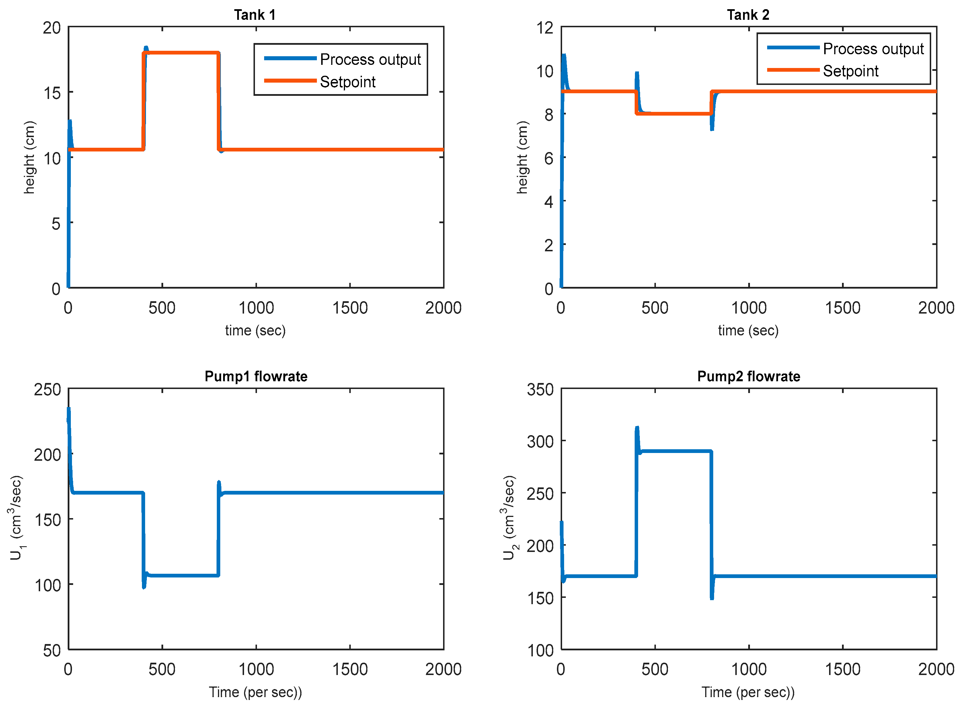
Shown in Figure 2 are the set-point tracking of the two lower tanks (Tank 1 and Tank 2) for closed loop simulations showing the controlled variables (h₁ and h₂) in addition to their respective manipulated variables, q₁ and q₂. The control scheme used for this closed loop simulation time of 2000 s is LMPC in a non-minimum phase.

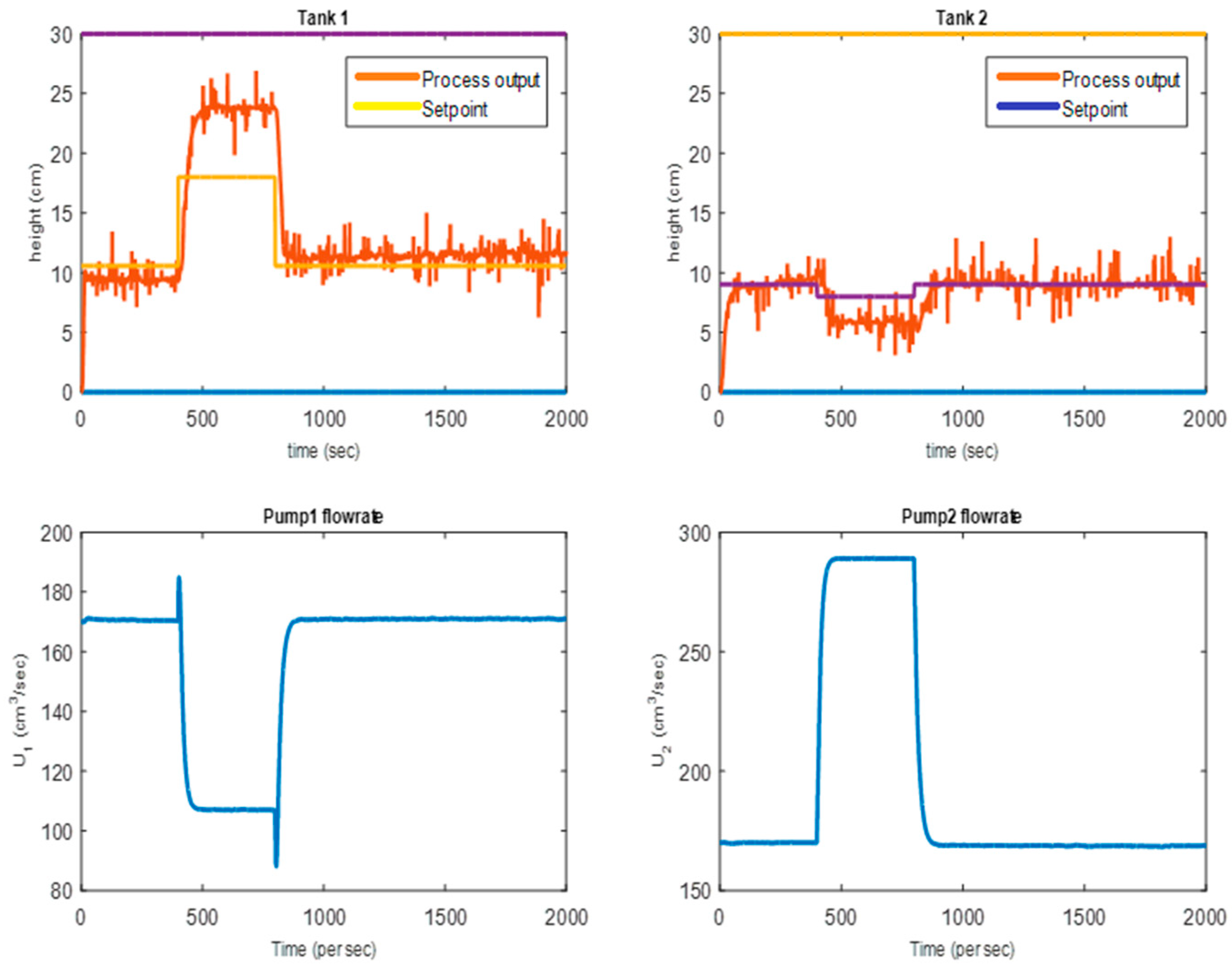
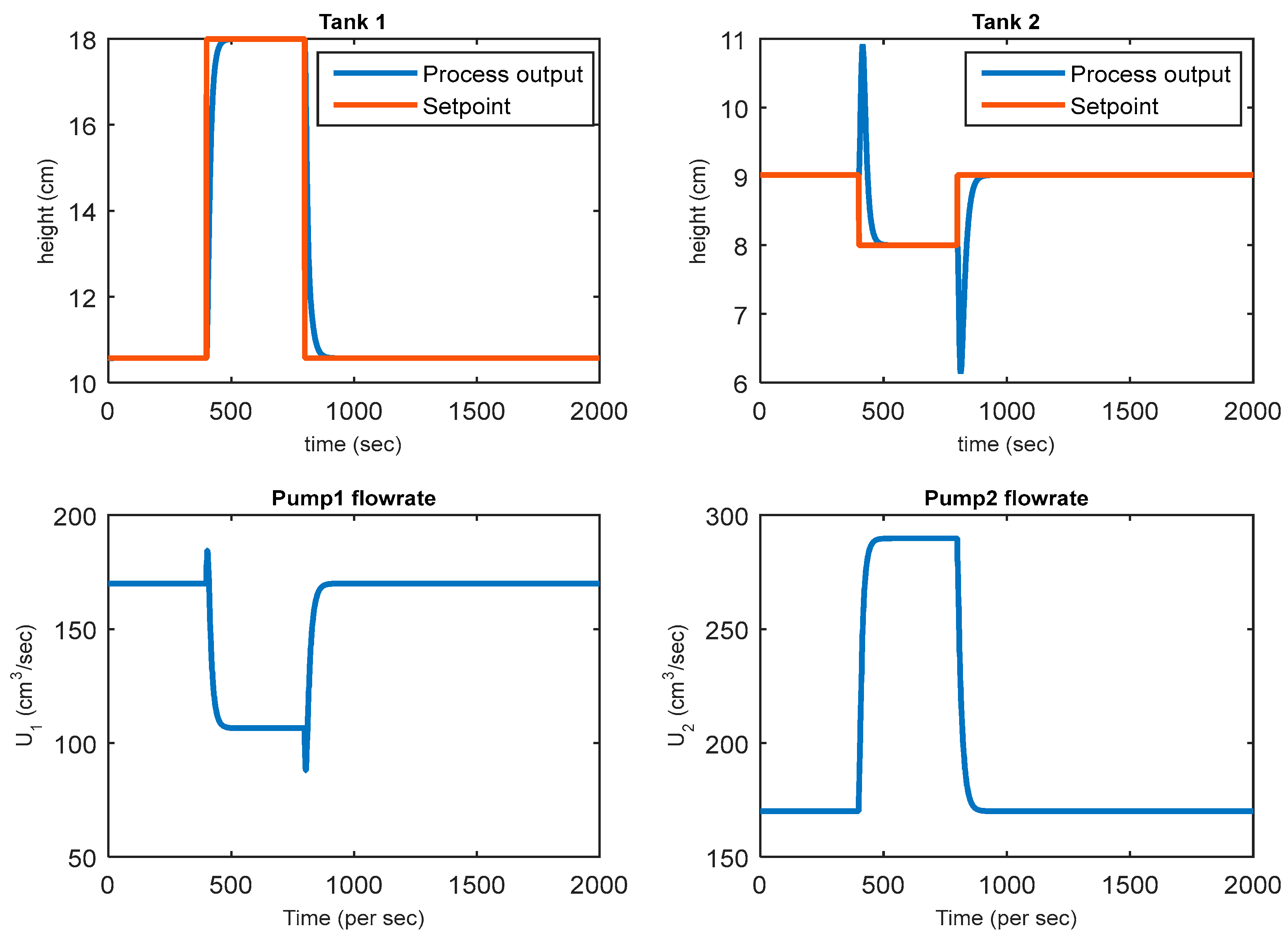
Also, Figure 3 shows the set-point tracking of Tank 1 and Tank 2 heights for closed loop simulations for a period of 2000 s using the designed NMPC in a non-minimum phase. The corresponding manipulated variables (q₁ and q₂) are shown as well.

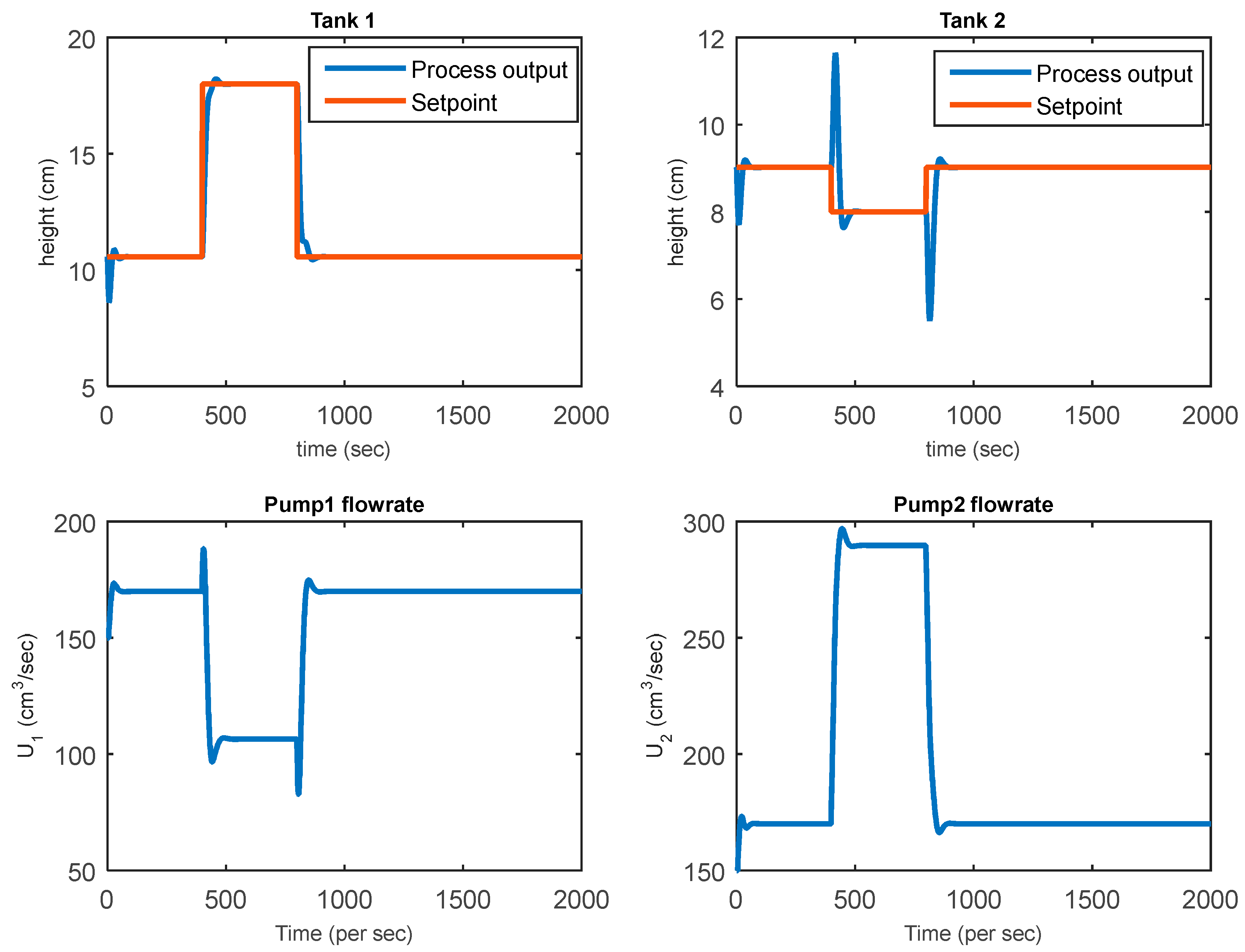
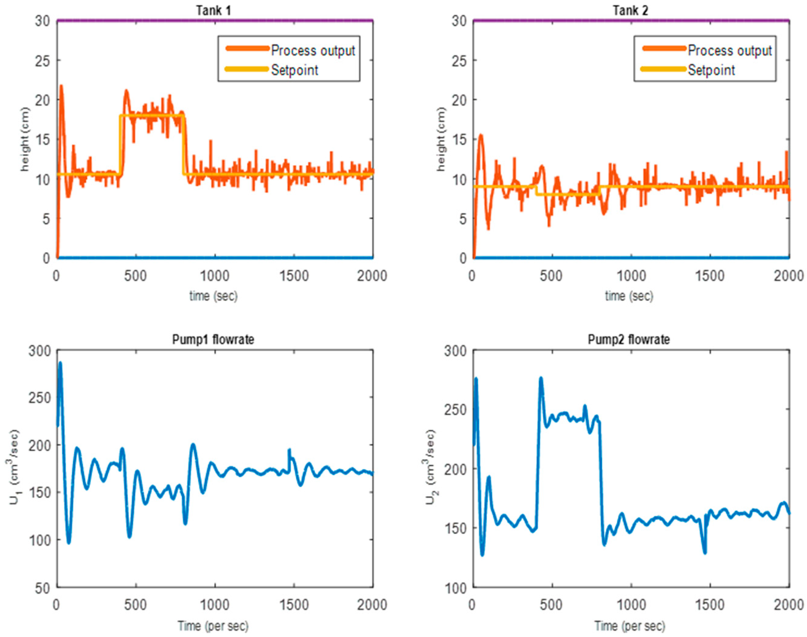
Figure 4 presents the designed NMPC augmented with an extended Kalman filter used to track setpoints, remove noise, and estimate the states. An inverse response was observed in the two lower tanks compared to the NMPC, where an inverse response was only observed in tank 2. Tank 1 and 2 levels for the closed-loop simulation for the three scenarios have negligible rise times and observed an inverse response with LMPC and NMPC-EKF.

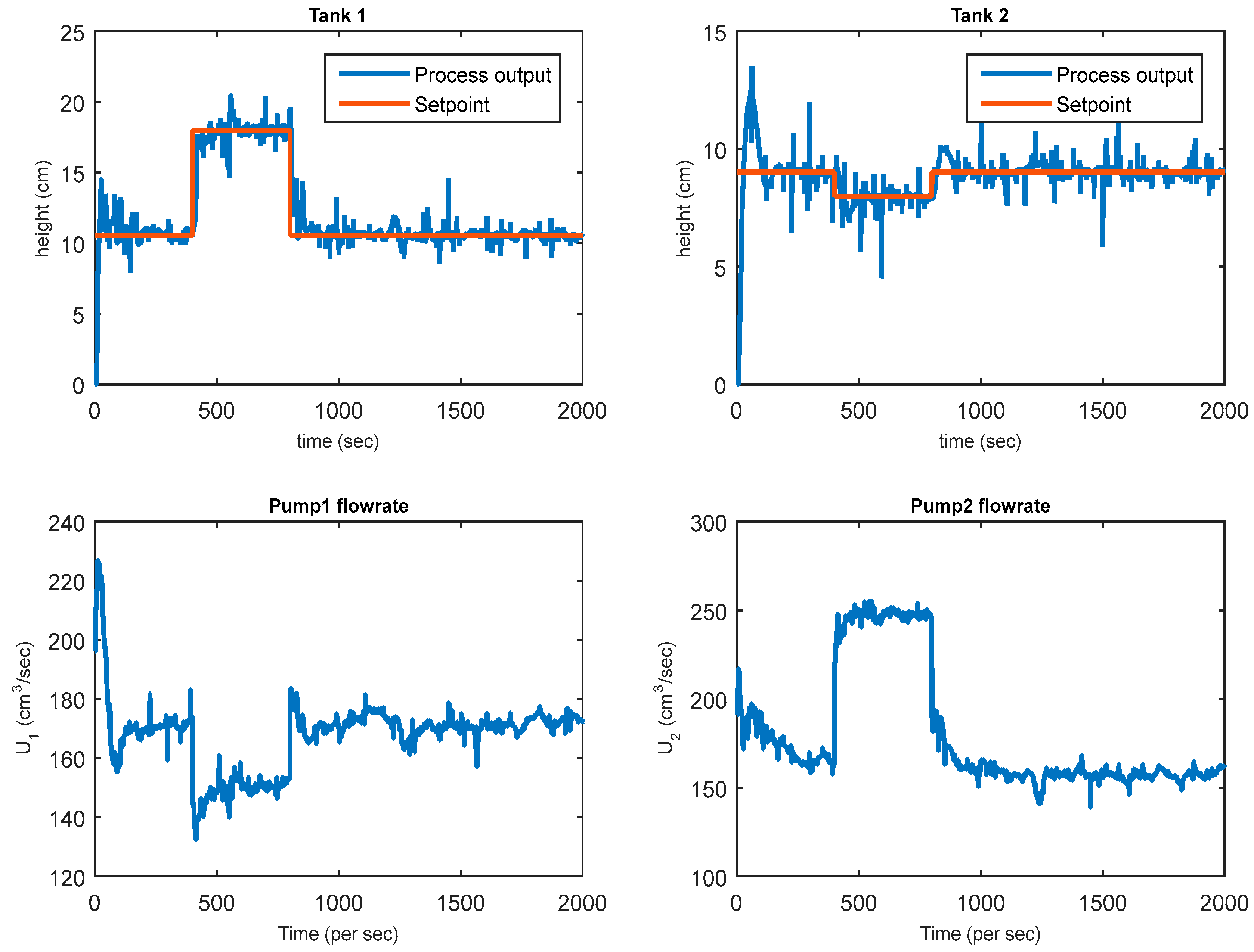
3.1. Real-Time Experimental Results

The closed-loop responses of tanks 1 and 2 obtained from the experimental implementation of the LMPC, NMPC, and NMPC-EKF in real time are shown in Figure 5, Figure 6 and Figure 7, respectively. The figures present the responses of the two lower tanks to setpoint changes using the designed controllers under non-minimum phase conditions. Manipulated input responses are shown.

It can be observed in Figure 5 for the tank 1 level response (h₁) that even though it tracked the setpoint before and after it was stepped, no inverse response was observed.

The tank 2 level response shows an apparently slight oscillatory response when the setpoints are stepped before finally tracking and settling. However, the tank 2 level response exhibited an inverse response and an overshoot.

In Figure 6, which involves the use of the NMPC controller, the tank 1 level response, unlike that obtained using LMPC, was found to settle without oscillation but overshot when the setpoint was stepped to 18 cm before dropping to continue the tracking process of the setpoint with mild undershoot at a setpoint of 9.021 cm.

The tank 2 level response exhibited a satisfactory tracking response, but when stepped to a lower value it undershot and finally tracked after 800 s in real time. In this case, an inverse response was observed to be significant.

With the NMPC controller augmented with EKF in Figure 7, perfect tracking of setpoints at every stage of the stepping was observed for tank 1 with visible inverse response. However, a significant overshoot occurred during the initial period, which finally settled after approximately 140 s.

For the tank 2 level, the response oscillated with decreasing amplitude towards settling before it was rapidly stepped at 400 s. The response finally settled after 1000 s.

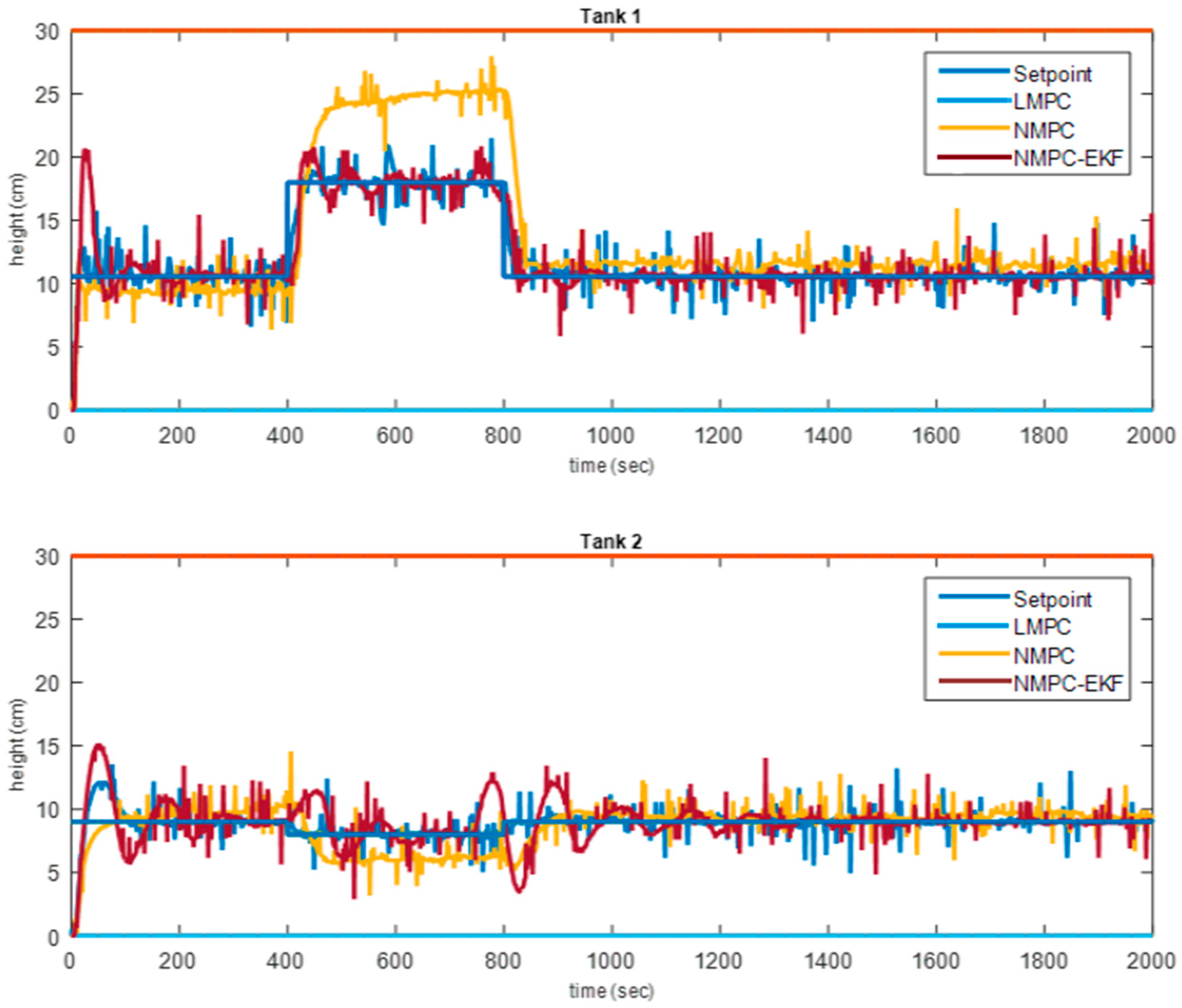
Figure 8 presents response comparison of the three controllers at the non-minimum phase.

3.2. Controllers’ Performance Indices

The performance of these controllers was judged based on their ability to track setpoints and the values of the IAE and ISE. Both controllers in the three scenarios tracked the setpoint, but at different rates. For instance, during the simulation, the LMPC, NMPC, and NMPC-EKF tracked the set point without overshooting. The LMPC seemed to be the best of the three during the simulation; it was able to track the setpoint smoothly and on time with an inverse response, smaller IAE and ISE, and with no overshoot for both outputs. The NMPC-EKF also tracked the setpoint but was not as smooth as the LMPC in the simulation. In addition, the performance of the controllers can be evaluated based on their overshoot, rising time, IAE, and ISE values.

Table 3. Lower tanks’ performance indices.

Index	LMPC		NMPC		NMPC-EKF
	Tank1	Tank2	Tank1	Tank2	Tank1	Tank2
IAE	66.74	40.13	259.1	218.2	222.5	215.2
Simulation ISE	326.4	47.6	1087	511.7	852	495.5
Rise Time	0	0	0	0	4.21	4.22
IAE	2691	1935	4091	1561	1375	2076
Real-Time ISE	7512	4990	18210	3893	4773	6705
Rise Time	11.89	12.78	13.77	14.41	14.62	14.88

presents the performance index for the simulation of the phase.

The responses from the experimental results showed that the LMPC gave smooth results, but when considering the performance indices, especially the integral errors of both the absolute and the square, NMPC-EKF seemed to be better.

The performance index values were larger than the comparative errors. Therefore, it can be inferred that the NMP is difficult to control, which supports what earlier researchers have observed.

4. Conclusions

In this study, the four-tank system was interfaced with a microcontroller board for direct digital control to measure the level of the two upper tanks and control the levels of the two lower tanks by manipulating the two inputs (pump flow rates). Owing to the strong interaction, the four-tank system is difficult to control in the non-minimum phase for conventional controllers; however, with the help of advanced controllers, better results are obtained.

Both linear and nonlinear MPC algorithms were designed and implemented in a four-tank experimental rig. The EKF was augmented in the algorithm to remove the offset from the NMPC.

In this study, based on the results obtained from the simulation of the Simulink models, NMPC controllers (augmented with EKF) were able to provide better control performance by tracking the setpoint smoothly with little overshoot and relatively stabilizing the system over time in comparison to the NMPC controller employed. However, it was discovered during the course of the experiment that the LMPC in real time gave a better result as compared to the NMPC simulation as the setpoint was tracked consistently with no overshoot; however, when considering performance indices, especially the integral errors of both the absolute and the square, NMPC-EKF proved to be better.

As an improvement on the advanced LMPC control technique, the NMPC was used to successfully control the experimental rig. However, based on real-time response, the NMPC controller failed to replicate the model accurately. Hence, state estimation with Kalman filtering was used to improve the performance.

References

- Johansson, K.H.; Nunes, J.L.R. A Multivariable Laboratory Process with an Adjustable Zero. Proc. Am. Conf. 1998, 4, 2045–2049. [Google Scholar]
- Grune, L.; Pannek, J. Nonlinear Model Predictive Control: Theory and Algorithms; Springer: New York, NY, USA, 2011. [Google Scholar]
- Qin, S.J.; Badgwell, T.A. A survey of industrial model predictive control technology. Control. Eng. Pract. 2003, 11, 733–764. [Google Scholar] [CrossRef]
- Van der Merwe, R. Sigma—Point Kalman Filters for Probabilistic Inference in Dynamic State—Space Models. Ph.D. Thesis, OGI School of Science and Engineering, Oregon Health and Science University, Portland, OR, USA, April 2004. [Google Scholar]
- Osunleke, A.S.; Deng, M.; Inoue, A.-A. CAGPC Controller Design for Systems with Input Windupand Disturbances. Int. J. Innov. Comput. Inf. Control. 2009, 5, 3517–3526. [Google Scholar]
- Bitmead, R.R.; Gevers, M.; Petersen, I.R.; Kaye, R.J. Monotonicity and stabilizability properties of solutions of the riccati difference equation: Propositions, lemmas, theorems, fallacious conjectures and counterexamples. Syst. Control. Lett. 1985, 5, 309–315. [Google Scholar] [CrossRef]
- Raff, T.; Huber, S.; Nagy, Z.K.; Allgower, F. Nonlinear Model Predictive Control of a Four Tank System: An Experimental Stability Study. In Proceedings of the 2006 IEEE International Conference on Control Applications, Munich, Germany, 4–6 October 2006. [Google Scholar]
- Johansson, K.H. The Quadruple-tank Process: A Multivariable Laboratory Process with an Adjustable Zero. IEEE Trans. Control. Syst. Technol. 2000, 8, 456–465. [Google Scholar] [CrossRef]
- Danica, R.M. Robust Control of Quadruple-tank Process. Inst. Control. Ind. Inform. 2008, 2, 231–238. [Google Scholar]
- Qamar, S.; Vali, U.; Reza, K. Multivariable Predictive PID for Quadruple Tank. World Acad. Sci. Eng. Technol. 2010, 43, 861–866. [Google Scholar]
- Bequette, W.B. Non-linear Model Predictive Control: A Personal Retrospective. Can. J. Chem. Eng. 2007, 85, 408–415. [Google Scholar] [CrossRef]