Abstract
Microscale photobioreactors for microalgae growth represent an interesting technology for fast data production and biomass characterization; however, the small scale poses severe monitoring challenges, as traditional methods cannot be used. Non-invasive techniques are therefore needed to quantify biomass concentration and other culture properties, for example, pigment composition. To this purpose, a soft sensing approach based on multivariate image regression is proposed to exploit RGB images and/or PAM-imaging chlorophyll fluorescence. Different PLS (Partial Least Squares) regression models are used to estimate: (a) biomass concentration from the features extracted by RGB indices and/or PAM-imaging chlorophyll fluorescence measurements; and (b) Chlorophyll a content per cell from the features extracted by RGB indices and biomass concentration measurements. Every single model is aimed at characterizing the microalgae culture at different light intensities during batch growth. Results show that the proposed monitoring approach is as accurate as traditional measurement approaches and may represent a promising methodology for fast and inexpensive monitoring of microscale photobioreactors.
1. Introduction
The development and application of microscale platforms, also called micro-photobioreactors (µPBR), for lab-scale microalgae cultivation has gained significant interest to overcome some limitations of traditional cultivation techniques, which are often time-consuming, high cost, labor-intensive and low throughput [1,2]. Microscale technologies are characterized by very small volumes (pL, nL, µL) and represent a powerful tool to enhance data quality and data production, because they allow for tight and rapid control of key operating variables, being also cheaper and compatible with high-throughput analyses. Recently proposed microscale technologies for microalgae were used for strain selection, size characterization and cell viability assessment [2]. On the other hand, a relevant drawback of microscale techniques is that the small cultivation volume of the device is not compatible with traditional lab-scale measurement protocols, thus requiring the development of ad hoc techniques. Even though lab-on-a-chip solutions may address this issue [3], they require a significant design effort and may adopt complex methods or expensive instrumentation. A monitoring technique suitable for a microscaled device must be online and noninvasive to avoid perturbing the system. Literature examples for the monitoring of µPBR typically rely on cell autofluorescence at a specific wavelength [4] or Chlorophyll fluorescence measurements [5,6]. However, chlorophyll fluorescence may lead to calibration problems due to significant measurement noise and self-absorbance and saturation issues. Image analysis can also be used as a monitoring technique, typically by coupling a microscope with an EMCCD camera, for example, to develop a single-cell tracking algorithm in µPBR built for single-layer cultivation [7], or to infer the growth rate through the surface area occupied by cells [8].
Alternatively, a simpler and faster approach is to utilize digital RGB images, in which each pixel consists of an array of red, green and blue intensity, in the range [0–255]. This monitoring method exploits the fact that color intensity is strictly linked to biomass concentration. However, as reviewed by Liu et al. [9], RGB images are rarely used to quantitatively describe microalgae and are mostly employed in larger-scale applications than µPBRs. Furthermore, constant light intensity is generally assumed. Usually, RGB images of microalgae samples are converted to grayscale and then correlated with biomass concentration [10,11]. A similar approach was used to estimate concentration via images of light distribution in a tubular photobioreactor [12]. It was also shown that the normalized intensity of the green channel can be correlated with the areal biomass concentration in the biofilm [13]. Interestingly, Su et al. [14] were able to estimate Chlorophyll a (Chl a) and lipids by establishing a correlation with RGB brightness; the methodology was validated in a real batch PBR.
In this work, a simple and fast soft sensing methodology based on multivariate image analysis [15] is proposed, to estimate the biomass concentration or Chl a content in a µPBR. A PLS (Partial Least Square) multivariate regression model was used to correlate color indices (mean and variance of each RGB channel) and/or chlorophyll fluorescence indices with biomass concentration in the µPBR. Adopting a similar approach, Chl a content was also estimated. Results from the cross-validated models showed that the methods represent a promising technique for the estimation of biomass concentration and chlorophyll content, thus paving the way towards an efficient, easy and inexpensive online monitoring of microalgae in microscale devices.
2. Materials and Methods
The cultivation of Scenedesmus obliquus was carried out in flat-plate batch PBRs at different light intensities. The biomass was then characterized (see Section 2.1.1) and transferred to a µPBR platform where images were collected. This is done to produce enough biomass to characterize microalgal concentration via traditional protocols (which otherwise would not be possible by using the µPBR platform only).
In the following, the cultivation methods, the assays and the mathematical models used to process the images will be described.
2.1. Microalgae Strain and Cultivation Method and Assays
A preinoculum of Scenedesmus obliquus 276.7 (obtained from SAG-Goettingen, Germany) was maintained in an Erlenmeyer flask with a BG11 medium. The preinoculum was kept at constant illumination of 80 μmol·m−2·s−1 and at a constant temperature of 23 ± 1 °C in a refrigerated incubator, in the flask was continuously injected with 5% CO2 enriched air. The medium BG11 was modified by adding HEPES 10 mM to prevent acidification due to continuous bubbling of 5% v/v CO2 enriched air [16]. A sample in the exponential phase was used as preinoculum and transferred in a polycarbonate flat-panel reactor, with a working volume of 150 mL to have an initial concentration of 5 × 10⁶ cells·mL−1 and working batch-wise. The optical path of the culture was 1.2 cm. At the bottom of the reactor, a sparger was placed through which 5% v/v CO2 enriched air was bubbled. Additional mixing was provided by a magnetic stirrer placed on the opposite side wall with respect to the illumination system. All reactors and media were previously autoclaved for 20 min at 121 °C to avoid any contamination. The flat-plate reactor was exposed to a constant continuous illumination of 35 (low light, LL), 150 (medium light, ML) and 950 μmol·m−2·s−1 (high light, HL) in biological duplicates (A and B) for each light condition with LED lamps. Incident light intensities were measured with an HD2012.1 photoradiometer (Delta Ohm, Italy), which measures the photosynthetically active radiation (PAR, 400–700 nm). Microalgae were cultivated in such reactors for five days in two parallel PBRs at a time.
2.1.1. Analytical Procedures
Biomass concentration was measured daily in doubles by using a Bürker chamber (HGB, Germany) while pH was measured with the HI9124 pH meter (Hanna Instruments, Italy) to check that the pH was between 7 and 8, the optimal range for cell viability. To extract the pigments, the biomass was ground with quartz powder and heated at 65 °C for 15 min with DMSO (dimethyl sulfoxide) [16]. The absorbance of the extracts was measured at 480, 649 and 665 nm by a UV-1900 UV-visible Spectrophotometer (Shimadzu, Japan), and concentrations of Chl a, Chl b and carotenoids were calculated with the following equations [17]:
Chl a = 12.19 · A665–3.45·A649
Chl b = 21.99 · A649–5.32·A665
Car = (1000 · A480–2.14 · Chl a–70.16·Chl b)/220
At the end of the batch curve, dry weight (DW) was measured by filtering a known volume of culture on pre-dried (15 min at 100 °C) cellulose acetate filters (0.45 µm, Whatman®, USA). The filtered biomass was then dried in the oven for 2 h at 100 °C.
Growth rates were calculated as the slope of the concentration profile in the logarithmic scale over time, during the exponential phase.
Photosynthetic efficiency is defined as the percentage of light used for microalgae growth with respect to the total received light [18]. It was calculated using the following equation:
where (g·L−1) is the increase in the concentration during the batch experiment, (L) is the reactor volume, LHV (22 KJ·g−1) is the lower heating value for S. obliquus [19], (m2) is the illuminated area of the reactor, (s) is the experiment duration and is the average energy of a mole of photons. was calculated from the photon spectrum of the lamp following the method described by Norton et al. [20] and is equal to 0.2139 J·µmol−1.
2.1.2. Sample Preparation
The culture from the flat-plate PBR was transferred into the µPBR sketched in Figure 1a. The µPBR was obtained with replica molding by curing PDMS (poly-di-methyl-siloxane) in a stereolitography-printed mold [6]. Eventually, the cured polymer was removed from the mold, obtaining the final µPBR device, fully compatible with biological applications [21]. Depending on the daily concentration in the flat-plate PBR, the cultivation broth (at concentration D0) was diluted to five different concentrations (namely D1, D2, D3, D4, D5). Concentrations ranged between D0 and 2.5 × 10⁶ cells·mL−1. Each concentration was placed in four different wells of the µPBR, whose position was chosen randomly for each experiment to increase the robustness of the model. The filled µPBR was eventually sealed with a 2 mm PDMS layer.
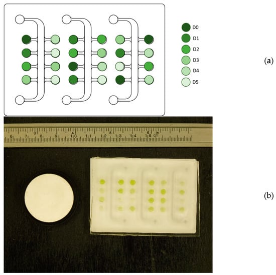
Figure 1.
(a) Representation of the scheme of sample dilution in the µPBR used for digital image acquisition [6]. Each well has a 4 mm diameter and 2 mm height. The dilutions of the culture from the PBR were inoculated in random positions. (b) Example of a raw image of the µPBR to be processed to extract features for the prediction model. The image corresponds to experiment HLB, day 4.
2.1.3. Digital Image Acquisition
The filled µPBR was placed in a black-painted wall box with a LED stripe, thus allowing a homogeneous illumination shading the device from environmental light noise. A digital camera (LUMIX DMC-TZ57, Panasonic, Japan) equipped with a 16 megapixel MOS sensor was mounted on a support to keep it in a fixed and stable position, in order to take pictures of the µPBR inside the black box. Length and white references were placed on the side of the µPBR and included in the image scene in such a way as to measure the pixel dimension and calibrate the white balance. The camera parameters, kept constant throughout all experiments, were as follows:
- ISO: 100;
- diaphragm opening: 6.3;
- exposure: 1/50 s;
- zoom: 3.5×;
- focal length: 15.1 mm.
One image was collected for each reactor every day. A raw image captured with the aforementioned protocol is shown in Figure 1b.
2.1.4. Fluorescence Measurement Acquisition
The same µPBR used for digital image acquisition was then used for chlorophyll fluorescence measurements with the PAM imaging OpenFluorCam FC 800 (Photon Systems Instruments, Drásov, Czech Republic) provided with its software FluorCam7. A dark adaption time of 20 min was required prior to performing the measurements to open all reaction centers [22,23]. The PAM-imaging instrument required to set the optimal parameters for the acquisition apparatus, which were:
- shutter = 1, corresponding to an aperture of 20 μs;
- sensitivity = 5, in a range 0–100;
- actinic light intensity (Act2) = 45, corresponding to 1150 μmol·m−2·s−1;
- pulse intensity (Super) = 35, corresponding to 1300 μmol·m−2·s−1.
The protocol, called Quenching Act2, required about 3 min and can be summarized as follows [24]:
- in the first 5 s of the protocol, minimum fluorescence is measured five times by using a measuring light;
- then, a saturating pulse (duration 800 ms) is used to calculate the maximum fluorescence and the variable fluorescence , where ;
- a dark phase of 17 s is used to relax all photosystems;
- actinic light is turned on for 70 s and after this, three saturating pulses (800 ms each) are produced at intervals of 10 s and another two pulses at an interval of 20 s. This allows the identification of the local maxima fluorescence due to progressive light acclimation, which is useful to describe NPQ dynamic (obtaining at different lights and , which is the steady-state value);
- actinic light is then turned off and this dark phase lasts until the end of the experiment. During this dark phase, three saturating pulses (800 ms each) are used at intervals of 30 s, identifying local fluorescence maxima allowing to calculate the relaxation of NPQ.
The software automatically calculates the following seven indices [23]: (maximum quantum efficiency of PSII), (maximum fluorescence in the dark-adapted state), , , , (instantaneous non-photochemical quenching during light adaptation) and (steady-state non-photochemical quenching in light) [24].
2.2. Mathematical Background
In this section, the mathematical methods used in this work are described.
2.2.1. PLS Regression Fundamentals
Partial Least Square (PLS) is one of the most used techniques in data analytics [25,26] to analyze chemical data for process control, fault detection and diagnosis [27]. This technique can also be applied to images for analysis, classification, segmentation and prediction [15]. For example, it was successfully used in the detection of food frauds [28], to classify inhomogeneous food matrices [29], in quality monitoring [30] and in process control [31]. In general, if is an autoscaled (i.e., each column has zero mean and unit variance) matrix of observations of predictors, and [] is the response matrix, PLS aims at finding a reduced number of latent variables, LV, that capture the part of the variance that best predicts . In particular, the two matrices can be rewritten in the form:
where A is the number of LV, [] and [] are the score matrices, [] and [] are the loading matrices, and are the residual matrices. W [] is the weight matrix and is used to project the original data into the new LV space. In this work, scores, loadings and weights were obtained through the SIMPLS algorithm and the number of LV was selected in order to minimize the cross-validation prediction error. Matlab 2018a with PLS Toolbox v. 8.6.2 (Eigenvector Research, Inc., USA) was used as software.
2.2.2. Image Pretreatment and Available Measurements
RGB images captured with the camera had a dimension of [3456 × 4608] pixels. To consider only pixels related to the culture and to avoid pixels at the border of the wells, which may be affected by edge effects, an inner ROI (region of interest) with a 50-pixel radius was selected, for a final image size of about 7500 pixels. For each ROI, it was possible to calculate the mean and variance () of the light intensities in each channel of the RGB image, thus characterizing each well. To summarize, for each well the following features were extracted:
- 6 color indices (CI) obtained from the digital image
- 7 fluorescence indices (FI) obtained from the PAM-imaging: , , , , , , ;
- biomass concentration obtained with manual count at the microscope: ;
- Chl a content obtained with the spectrophotometric assay: Chl a.
A preliminary analysis showed that including the data from the first two days of the batch was detrimental for model performance (in the first two days photoacclimation phenomena strongly affect cultivation, see Section 3.1). For this reason, only the last three days of the batch campaigns were considered, for a total number of wells (e.g., observations) of . Data from different batches were organized by rows, similar to the feature-wise unfolding approach [32]. Since all the measurements were performed in double, this allowed increasing the number of observations up to 144 to increase model robustness. We can define two matrices that constitute the predictor matrix of the model: one containing the features extracted from the RGB images, namely a color matrix [144 × 6], and one containing fluorescence indices [144 × 7]. The predictive models will be indicated as M[|], where M is the model ID, while in the squared brackets are listed the concatenated matrices (hence, the features) used in the predictor matrix and the predicted variable .
2.2.3. PLS for Biomass Concentration Estimation
The models built in this section aim at estimating biomass concentration in the µPBR wells, regardless of the incident light used in the experiment, or the day in which the image was collected. In this case, only indices obtained from the wells at D0 were used (e.g., the original culture sampled from the PBR as in Figure 1a). The matrix structure is represented in Figure 2. In particular, the following models were tested:
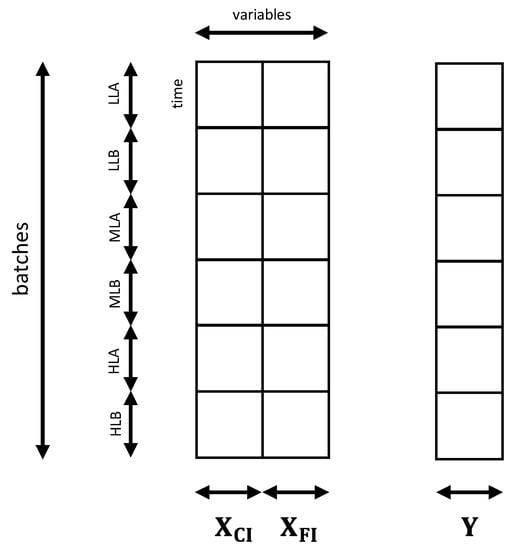
Figure 2.
Matrices used to build the PLS models to estimate biomass concentration. The predictor matrix was built concatenating and depending on the model. The response matrix [144 × 1] consisted of the biomass concentration or in its logarithm, depending on the model.
- C[Cx]: only color indices were used to predict biomass concentration;
- C[Cx]: CI and FI were used in the prediction of the concentration;
- C[ln(Cx)]: only color indices were used to predict the logarithm of the concentration;
- C[ln(Cx)]: only fluorescence indices were used to predict the logarithm of the concentration;
- C[ln(Cx)]: CI and FI were used in the prediction of the logarithm of the concentration.
2.2.4. PLS for Chlorophyll Content Estimation
The models built in this section aim at estimating Chl a content (pg·cell−1), regardless of the incident light used in the experiment, or the day in which the image was collected. Only the wells at D0 were used. The matrix structure is shown in Figure 3. For this purpose, the biomass concentration was evaluated as an additional predictor, organized in the vector [144 × 1]. In particular, the following models were tested:
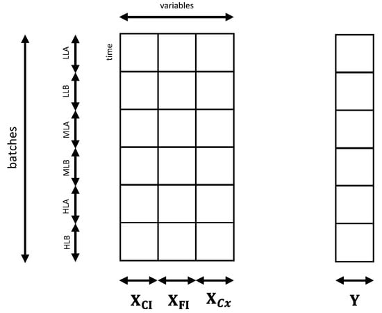
Figure 3.
Matrices used to build the PLS models to estimate Chl a content. The predictor matrix was built concatenating , and the vector containing biomass concentration depending on the model. The response matrix [144 × 1] consisted of the Chl a content.
- P[Chla]: only color indices were used to predict Chl a content;
- P[Chla]: color indices and biomass concentration were used to predict Chl a content;
- P[|Chla]: color indices, biomass concentration and fluorescence indices were used to predict Chl a content.
2.2.5. Assessing Model Performance
Cross-validation was performed by iterating 100 times the validation procedure in which 90% of the observations were randomly selected for calibration, while the remaining observations were used for validation. Model performance was assessed by calculating the average relative and average absolute errors on validation:
where is the experimental value of the biomass concentration (or pigment content) and the predicted value; is the total number of validated samples. To assess the fitting performance of the different models, the average SSR (sum of squared residuals) was calculated.
3. Results
3.1. Batch Culture Evolution
Here, the batch cultures used to set up the models are discussed. Growth curves at different impinging light intensities are reported in Figure 4, in which a typical batch growth trend can be observed, with an initial lag phase, an exponential phase and eventually a stationary phase for HL experiments only. The calculated growth rates (Table 1) were increasing with light as expected; however, the increase of growth rate was not linear, suggesting possible saturation under HL. This is further confirmed by the photosynthetic efficiency, which drastically decreased under HL, confirming a less efficient conversion of light into biomass.
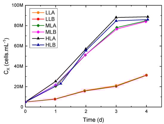
Figure 4.
Growth curves in flat-plate PBR under different continuous illumination in two biological replicates (A and B): 35 (low light, LL), 150 (medium light, ML) and 950 μmol·m−2·s−1 (high light, HL).

Table 1.
Growth rates, dry weights and photosynthetic efficiency obtained in the flat-plate PBRs.
As reported in Figure 5, during the initial days of the batches, an adjustment of Chl a was observed due to photoacclimation from the preinoculum condition to the new growth conditions in the flat-plate PBR. Eventually, Chl a reached a pseudo-stationary condition starting from day 2. While LL and ML experiments reached a similar value, HL experiments had a reduced Chl a content per cell. As a consequence, HL experiments had a higher ratio Car/Chl a, which is a common photoprotective response [33]. A similar conclusion can be drawn by looking at the trends in Figure 6: the LL and ML experiments show values above 0.6 for all the samples (for healthy unstressed cells this value is usually in the range 0.6–0.8 [34]), while for cultures exposed at high light intensity a lower value was measured, suggesting possible photoinhibition. To observe variability fluorescence measurements, was measured for a sample and its dilution. The sample was collected at the end of the exponential phase and transferred to the µPBR together with its five dilutions as described in the previous section (Figure 7). Linearity in was found limited for a very small and narrow concentration range and a certain variability was always present. The range is strictly dependent on the specific PAM-imaging settings and protocol used [6], thus making the usage of such measurements for concentration estimation a complex task. In addition, at higher concentrations, self-absorbance and saturation issues may arise [5], which pose additional challenges to correct calibration.
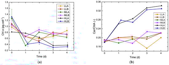
Figure 5.
Evolution of pigment content over time. Error bars are the standard deviations between duplicates. (a) Chl a content per cell. The average standard deviation is about 0.06 pg·cells−1, however in some samples the error is higher, up to 0.12–0.15 pg·cells−1. (b) Carotenoids/Chl a ratio over time.
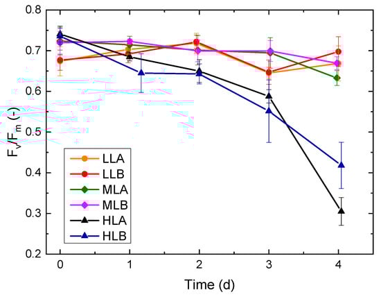
Figure 6.
Trend of (e.g., maximum quantum efficiency of PSII), over time for the six batch experiments.
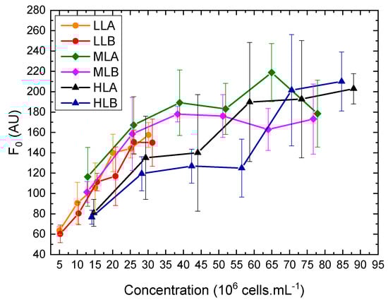
Figure 7.
Dependence of on biomass concentration of samples collected at the end of the exponential phase and their dilutions, for batch experiments. Error bars are the standard deviation among four wells at the same concentration.
3.2. Results of the Biomass Concentration Estimation
The models described in Section 2.2.3 were used to predict biomass concentration. Note that the same model is used to predict biomass concentration at three different light intensities and at three different times (days) in the dynamic batch cultivation curve.
Detailed results are reported in Table 2. At first, it can be seen that using the logarithmic model C[ln(Cx)] helps reducing the average relative error with respect to C[Cx], while the average absolute error remains almost unchanged. Comparison between C[ln(Cx)] and C[ln(Cx)] confirmed that using only fluorescence measurements as predictors may lead to large errors in the prediction of biomass concentration. For the sake of completeness, it must be noticed that the biomass concentration range is quite wide (10–90 × 106 cell·mL−1) with respect to ranges usually adopted in literature for the application of fluorescence measurements, and saturation phenomena may be present. Model C[ln(Cx)] allowed for the smallest average relative error by using all the available predictors, namely CI and FI. Parity plots for all models are reported in Figure 8. Here the effect of the logarithm transformation in the predictions can be noticed. In fact, the logarithm slightly improves predictions at lower concentrations, while at higher concentrations predictions are more scattered, suggesting that a linear dependence would be preferable at these values. Both relative and absolute error distributions for model C[ln(Cx)] can be observed in Figure 9. Only a small subset of samples has a relative error larger than 20% and an absolute error larger than 15 × 106 cell·mL−1, while the average relative error is 18.74% and the average absolute error is 9.51 × 10⁶ cell·mL−1 (comparable to experimental measurements as also reported in the literature [35]). However, the rapidity of the response that could be obtained via image analysis makes it a promising and effective technique for fast estimation of a sample concentration.
Table 2.
Performance of the models used to estimate biomass concentration. Note that, when the logarithm is predicted, the final values were converted back into concentration and errors were calculated.
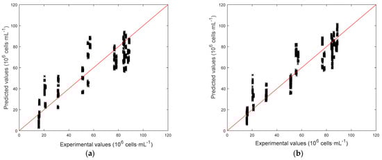
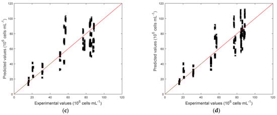
Figure 8.
Parity plots for the models predicting the biomass concentrations. (a) C[Cx], SSR = 30.43. (b) C[Cx], SSR = 16.08. (c) C[ln(Cx)], SSR = 22.33. (d) C[ln(Cx)], SSR = 14.05.
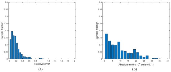
Figure 9.
Model C[ln(Cx)]. (a) Relative error distributions. (b) Absolute error distributions.
In view of the results above, where only wells at D0 were used for calibration and validation, an additional model was built where the number of variables was increased by using the features extracted from diluted wells (Figure 10). The best prediction performances were obtained by using three dilutions, namely D1, D2 and D3, for example, removing noisy dilutions. Matrix was therefore increased to (6 + 7)·4 = 52 predictors. The target concentration was again the logarithm of wells at D0 and the performance of this model D[ln(Cx)] are summarized in Table 3. We can see in Figure 11 that errors are significantly smaller with respect to the ones obtained with C[ln(Cx)]. In addition, by looking at the parity plot in Figure 12, predictions at the highest concentrations were improved with respect to Figure 8d. In general, this model was very effective at characterizing biomass concentration in a wide range, although the need to provide several dilutions of the culture makes its application on µPBR potentially problematic (although it can represent a viable solution at a larger scale).
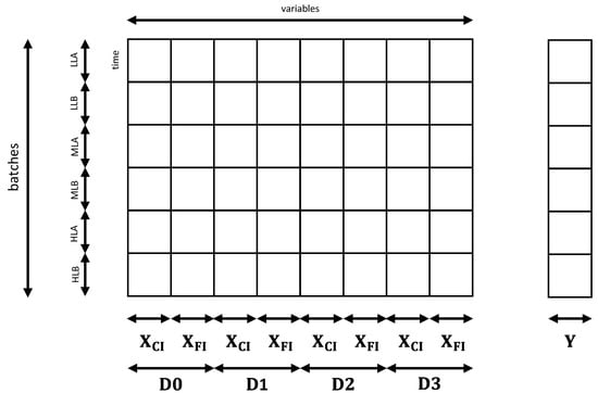
Figure 10.
Sketch of the new predictor matrix to improve biomass concentration prediction. The number of variables was increased by using features extracted from wells at three additional dilutions of the original culture D0. The response consisted of the logarithm of the concentration.
Table 3.
Performance of the model that used dilutions to estimate biomass concentration.
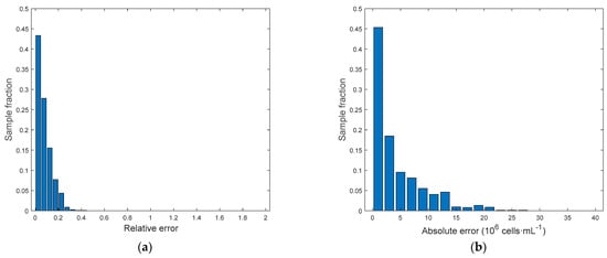
Figure 11.
Model D[ln(Cx)]. (a) Relative error distribution. (b) Absolute error distribution.
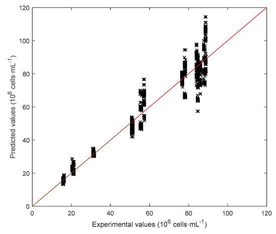
Figure 12.
Parity plot for model D[ln(Cx)], SSR = 1.62.
3.3. Results of the Chl a Estimation
In this section, the goal is predicting the Chl a content [pg·cell−1]. Also, in this case, the model aim at predicting pigment content at 3 different light intensities and at 3 days in the dynamic batch cultivation curve. However, it is necessary to acknowledge that the technique based on pigments extraction and spectrophotometric measurements presents a significant variability (Figure 5a). In fact, the standard deviation of pigment assays performed in doubles ranges from 0.01 to 0.12 pg·cell−1 with an average of 0.05 pg·cell−1. Model P[Chla] with only color indices seems underperforming as its average relative error is quite high. Biomass concentration was then added to take into account the different chlorophyll content depending on the concentration in a well. In fact, model P[Chla] allowed decreasing the average relative error significantly. It can be observed that model P[|Chla] in which FI were added, did not perform significantly better. In conclusion, P[Chla] is able to represent adequately all the observations with a reasonable error, which is comparable to the traditional assay error (Figure 5). By looking at the error distributions (Figure 13), we can see that most samples are characterized by very low errors. From the parity plot (Figure 14) it is possible to notice that the pigment duplicate measurements present a significant variability (points are quite spread along x-axis), affecting the prediction accuracy of the model. Detailed results concerning the model performances in estimating Chl a are reported in Table 4.
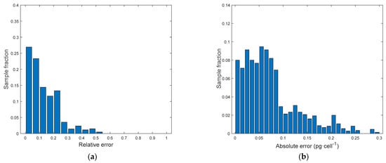
Figure 13.
Model P[Chla]. (a) Relative error distribution. (b) Absolute error distribution.
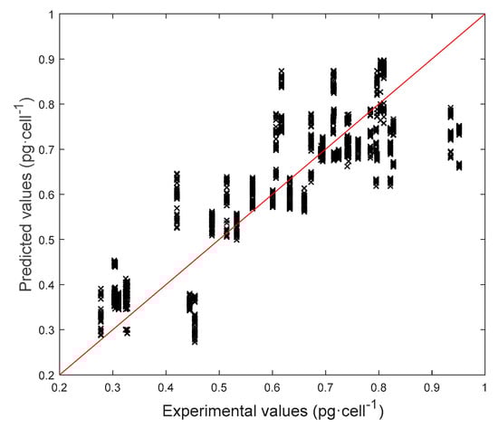
Figure 14.
Parity plot for model P[Chla], SSR = 33.76.
Table 4.
Performance of the models used to estimate Chl a content.
4. Conclusions
Multivariate image analysis has been assessed aimed at estimating biomass concentration or Chlorophyll a content in µPBRs.
Models built to predict biomass concentration led to promising results as the combined exploitation of color and fluorescence indices allows one to obtain an average relative error of about 18%, which is comparable to experimental measurements. A more complex but accurate model was built by including data based on diluted samples of the original culture. Although this methodology may not be suitable for a direct application on µPBR, it may represent a promising approach to reduce the operator effort and to avoid microscope counting.
Models built to predict Chl a also led to interesting results. In this case, however, information on biomass concentration may have to be combined with color indices in order to reach acceptable accuracy in the estimates of pigment content in a µPBR. The approach may represent a valuable substitute for traditional lab assays, which are typically time-consuming and labor-intensive.
These preliminary results also suggest that a larger dataset of images of culture at different illumination or conditions would be beneficial to increase model robustness and precision. Future work will aim at exploring different color spaces, such as HSL (Hue, Saturation, Lightness), CIELAB or RG chromaticity to assess if they may lead to an improvement in the monitoring performance.
Author Contributions
Experiments and data treatment: A.G. Algorithm: A.G., C.C. Conceptualization, F.B., E.S., P.F., C.C. Writing—original draft preparation, C.C.; writing—review and editing, E.S., P.F., F.B.; supervision, F.B. All authors have read and agreed to the published version of the manuscript.
Funding
This research received no external funding.
Data Availability Statement
Data available on request due to restrictions.
Conflicts of Interest
The authors declare no conflict of interest.
List of Symbols
| Abbreviations | |
| Car | Carotenoids |
| Chl a | Chlorophyll a |
| Chl b | Chlorophyll b |
| CI | Color indices |
| D0, …, D5 | Dilutions |
| DMSO | Dimethyl sulfoxide |
| DW | Dry weight |
| EMCCD | Electron-multiplying charged-coupled device |
| FI | Fluorescence indices |
| HL | Experiments at high light |
| HSL | Hue saturation lightness color space |
| LHV | Lower heating value |
| LL | Experiments at low light |
| LV | Latent variables |
| ML | Experiments at medium light |
| NPQ | Non-photochemical quenching |
| PAM | Pulse amplitude modulation |
| PAR | Photosynthetically active region |
| PBR | Photobioreactor |
| PDMS | poly-di-methyl-siloxane |
| PLS | Partial least squares |
| PSII | Photosystem II |
| ROI | Region of interest |
| SSR | Sum of squared residuals |
| µPBR | Micro-photobioreactor |
| Roman symbols | |
| Latent variable | |
| Biomass concentration | |
| Average absolute error | |
| Average energy of a mole of photons | |
| Average relative error | |
| Minimum fluorescence | |
| Maximum fluorescence | |
| Variable fluorescence | |
| Incident light intensity | |
| Means of red, green and blue channels | |
| Number of observations | |
| Number of variables | |
| Number of responses | |
| Variances of red, green and blue channels | |
| Greek letters | |
| µ | Growth rate |
| Matrices and arrays | |
| Residual matrices | |
| Loadings matrix of | |
| Loadings matrix of | |
| Scores matrix of | |
| Scores matrix of | |
| Weight matrix | |
| Predictor matrix | |
| Color indices predictors | |
| Biomass concentration predictor | |
| Fluorescence indices predictors |
References
- Juang, Y.-J.; Chang, J.-S. Applications of microfluidics in microalgae biotechnology: A review. Biotechnol. J. 2016, 11, 327–335. [Google Scholar] [CrossRef] [PubMed]
- Kim, H.S.; Devarenne, T.P.; Han, A. Microfluidic systems for microalgal biotechnology: A review. Algal Res. 2018, 30, 149–161. [Google Scholar] [CrossRef]
- Pierobon, S.C.; Cheng, X.; Graham, P.J.; Nguyen, B.; Karakolis, E.G.; Sinton, D. Emerging microalgae technology: A review. Sustain. Energy Fuels 2018, 2, 13–38. [Google Scholar] [CrossRef]
- Zheng, G.; Wang, Y.; Wang, Z.; Zhong, W.; Wang, H.; Li, Y. An integrated microfluidic device in marine microalgae culture for toxicity screening application. Mar. Pollut. Bull. 2013, 72, 231–243. [Google Scholar] [CrossRef]
- Perin, G.; Cimetta, E.; Monetti, F.; Morosinotto, T.; Bezzo, F. Novel micro-photobioreactor design and monitoring method for assessing microalgae response to light intensity. Algal Res. 2016, 19, 69–76. [Google Scholar] [CrossRef]
- Castaldello, C.; Sforza, E.; Cimetta, E.; Morosinotto, T.; Bezzo, F. Microfluidic Platform for Microalgae Cultivation under Non-limiting CO2 Conditions. Ind. Eng. Chem. Res. 2019, 58, 18036–18045. [Google Scholar] [CrossRef]
- Luke, C.S.; Selimkhanov, J.; Baumgart, L.; Cohen, S.E.; Golden, S.S.; Cookson, N.A.; Hasty, J. A Microfluidic Platform for Long-Term Monitoring of Algae in a Dynamic Environment. ACS Synth. Biol. 2016, 5, 8–14. [Google Scholar] [CrossRef]
- Westerwalbesloh, C.; Brehl, C.; Weber, S.; Probst, C.; Widzgowski, J.; Grünberger, A.; Pfaff, C.; Nedbal, L.; Kohlheyer, D. A microfluidic photobioreactor for simultaneous observation and cultivation of single microalgal cells or cell aggregates. PLoS ONE 2019, 14, e0216093. [Google Scholar] [CrossRef] [Green Version]
- Liu, J.Y.; Zeng, L.H.; Ren, Z.H. The application of spectroscopy technology in the monitoring of microalgae cells concentration. Appl. Spectrosc. Rev. 2020, 56, 171–192. [Google Scholar] [CrossRef]
- Córdoba-Matson, M.V.; Gutiérrez, J.; Porta-Gándara, M.Á. Evaluation of Isochrysis galbana (clone T-ISO) cell numbers by digital image analysis of color intensity. J. Appl. Phycol. 2010, 22, 427–434. [Google Scholar] [CrossRef]
- Sarrafzadeh, M.H.; La, H.J.; Lee, J.Y.; Cho, D.H.; Shin, S.Y.; Kim, W.J.; Oh, H.M. Microalgae biomass quantification by digital image processing and RGB color analysis. J. Appl. Phycol. 2015, 27, 205–209. [Google Scholar] [CrossRef]
- Jung, S.K.; Lee, S.B. In situ monitoring of cell concentration in a photobioreactor using image analysis: Comparison of uniform light distribution model and artificial neural networks. Biotechnol. Prog. 2006, 22, 1443–1450. [Google Scholar] [CrossRef] [PubMed]
- Murphy, T.E.; Macon, K.; Berberoglu, H. Multispectral image analysis for algal biomass quantification. Biotechnol. Prog. 2013, 29, 808–816. [Google Scholar] [CrossRef] [PubMed]
- Su, C.H.; Fu, C.C.; Chang, Y.C.; Nair, G.R.; Ye, J.L.; Chu, I.M.; Wu, W.T. Simultaneous estimation of chlorophyll a and lipid contents in microalgae by three-color analysis. Biotechnol. Bioeng. 2008, 99, 1034–1039. [Google Scholar] [CrossRef] [PubMed]
- Prats-Montalbán, J.M.; de Juan, A.; Ferrer, A. Multivariate image analysis: A review with applications. Chemom. Intell. Lab. Syst. 2011, 107, 1–23. [Google Scholar] [CrossRef]
- Gris, B.; Morosinotto, T.; Giacometti, G.M.; Bertucco, A.; Sforza, E. Cultivation of Scenedesmus obliquus in Photobioreactors: Effects of Light Intensities and Light–Dark Cycles on Growth, Productivity, and Biochemical Composition. Appl. Biochem. Biotechnol. 2014, 172, 2377–2389. [Google Scholar] [CrossRef]
- Wellburn, A.R. The Spectral Determination of Chlorophylls a and b, as well as Total Carotenoids, Using Various Solvents with Spectrophotometers of Different Resolution. J. Plant Physiol. 1994, 144, 307–313. [Google Scholar] [CrossRef]
- Watanabe, Y.; Hall, D.O. Photosynthetic CO2 conversion technologies using a photobioreactor incorporating microalgae—Energy and material balances. Energy Convers. Manag. 1996, 37, 1321–1326. [Google Scholar] [CrossRef]
- Sforza, E.; Urbani, S.; Bertucco, A. Evaluation of maintenance energy requirements in the cultivation of Scenedesmus obliquus: Effect of light intensity and regime. J. Appl. Phycol. 2015, 27, 1453–1462. [Google Scholar] [CrossRef]
- Norton, M.; Gracia Amillo, A.M.; Galleano, R. Comparison of solar spectral irradiance measurements using the average photon energy parameter. Sol. Energy 2015, 120, 337–344. [Google Scholar] [CrossRef]
- Velve-Casquillas, G.; Le Berre, M.; Piel, M.; Tran, P.T. Microfluidic tools for cell biological research. Nano Today 2010, 5, 28–47. [Google Scholar] [CrossRef] [Green Version]
- Maxwell, K.; Johnson, G.N. Chlorophyll fluorescence—A practical guide. J. Exp. Bot. 2000, 51, 659–668. [Google Scholar] [CrossRef]
- Murchie, E.H.; Lawson, T. Chlorophyll fluorescence analysis: A guide to good practice and understanding some new applications. J. Exp. Bot. 2013, 64, 3983–3998. [Google Scholar] [CrossRef] [PubMed] [Green Version]
- FluorCam Instruction Manual, version 2.0; Photon Systems Instruments: Drasov, Czech Republic, 2012.
- Geladi, P.; Kowalski, B.R. Partial least-squares regression: A tutorial. Anal. Chim. Acta 1986, 185, 1–17. [Google Scholar] [CrossRef]
- Wise, B.M.; Gallagher, N.B. The process chemometrics approach to process monitoring and fault detection. J. Process Control 1996, 6, 329–348. [Google Scholar] [CrossRef]
- Kourti, T. Application of latent variable methods to process control and multivariate statistical process control in industry. Int. J. Adapt. Control Signal Process. 2005, 19, 213–246. [Google Scholar] [CrossRef]
- Ottavian, M.; Fasolato, L.; Serva, L.; Facco, P.; Barolo, M. Data Fusion for Food Authentication: Fresh/Frozen–Thawed Discrimination in West African Goatfish (Pseudupeneus prayensis) Fillets. Food Bioprocess Technol. 2014, 7, 1025–1036. [Google Scholar] [CrossRef]
- Antonelli, A.; Cocchi, M.; Fava, P.; Foca, G.; Franchini, G.C.; Manzini, D.; Ulrici, A. Automated evaluation of food colour by means of multivariate image analysis coupled to a wavelet-based classification algorithm. Anal. Chim. Acta 2004, 515, 3–13. [Google Scholar] [CrossRef]
- Facco, P.; Masiero, A.; Beghi, A. Advances on multivariate image analysis for product quality monitoring. J. Process Control 2013, 23, 89–98. [Google Scholar] [CrossRef]
- Duchesne, C.; Liu, J.J.; MacGregor, J.F. Multivariate image analysis in the process industries: A review. Chemom. Intell. Lab. Syst. 2012, 117, 116–128. [Google Scholar] [CrossRef]
- Kourti, T. Multivariate dynamic data modeling for analysis and statistical process control of batch processes, start-ups and grade transitions. J. Chemom. 2003, 17, 93–109. [Google Scholar] [CrossRef]
- Meneghesso, A.; Simionato, D.; Gerotto, C.; La Rocca, N.; Finazzi, G.; Morosinotto, T. Photoacclimation of photosynthesis in the Eustigmatophycean Nannochloropsis gaditana. Photosynth. Res. 2016, 129, 291–305. [Google Scholar] [CrossRef] [PubMed]
- Masojídek, J.; Vonshak, A.; Torzillo, G. Chlorophyll a Fluorescence in Aquatic Sciences: Methods and Applications; Suggett, D.J., Prášil, O., Borowitzka, M.A., Eds.; Springer: Dordrecht, The Netherlands, 2010; ISBN 978-90-481-9267-0. [Google Scholar]
- Camacho-Fernández, C.; Hervás, D.; Rivas-Sendra, A.; Marín, M.P.; Seguí-Simarro, J.M. Comparison of six different methods to calculate cell densities. Plant Methods 2018, 14, 30. [Google Scholar] [CrossRef] [PubMed] [Green Version]
Publisher’s Note: MDPI stays neutral with regard to jurisdictional claims in published maps and institutional affiliations. |
© 2021 by the authors. Licensee MDPI, Basel, Switzerland. This article is an open access article distributed under the terms and conditions of the Creative Commons Attribution (CC BY) license (https://creativecommons.org/licenses/by/4.0/).