Artificial Intelligence-Based Models for Wax Deposition Prediction in Oil Pipelines: Potential, Challenges, and Future Directions

Abstract

Wax deposition in pipelines is a major issue in the oil and gas industry. Estimating the main characteristics of the wax deposits is crucial in mitigating their negative impact. Thus, developing predictive models plays an important role in managing wax deposition. Artificial intelligence (AI)-based models have proven their effectiveness and accuracy, along with several advantages such as ease of use, flexibility, and adaptability. This paper presents a comprehensive review of 41 primary studies reporting over 100 individual AI-based models used for wax deposition prediction, including support vector machines (SVMs), feedforward neural networks (multilayer perceptron, RBFNN, cascade-forward, and others), neuro-fuzzy systems, and tree-based models, together with hybrid and metaheuristic-optimized variants. In addition, AI-based models that integrate multiple single-model predictors or optimization techniques were also reviewed. This paper discusses the underlying principles, applications, strengths, and limitations of these AI-based prediction techniques and concludes with an outlook on future research directions in AI-driven wax deposition prediction. According to the reviewed papers, and by analyzing the errors reported, AI-based models can successfully predict the wax deposition rate, deposited weight, thickness, wax appearance temperature (WAT), and wax disappearance temperature (WDT). AI-based models have high potential to compete with conventional models and efficiently contribute to wax deposition control and management. This review finds that although these models routinely report high accuracy (R² > 0.95), such results are typically obtained on small, frequently reused datasets with limited validation. While gradient-boosting tree ensembles are the most frequent winners in recent head-to-head comparisons, no single model family is consistently superior across prediction targets.

1. Introduction

Crude oil is a complex mixture of hydrocarbons that vary in composition and molecular structure. In addition to hydrocarbons, it contains other elements such as sulfur, nitrogen, oxygen, and trace amounts of metal compounds. When crude oil has a high concentration of long-chain paraffin waxes, including both normal (n-alkanes) and iso-alkanes, along with aromatics, cycloalkanes, resins, and asphaltenes, it is classified as waxy crude oil [1]. These high-molecular-weight paraffinic compounds, which have a high number of carbon atoms from 18 to 75, are characterized by their high boiling point and ability to deposit as solid wax crystals [2,3]. High-molecular-weight compounds in crude oil remain dissolved under reservoir pressure and temperature conditions. However, during extraction and transportation, the temperature drops and may reach the wax appearance temperature (WAT), defined as the temperature at which the first wax crystals precipitate out of the liquid phase [4]. Wax in crude oil can be broadly classified into two main types: macrocrystalline wax and microcrystalline wax. Macrocrystalline wax consists primarily of straight-chain alkanes (n-alkanes) that form large, needle-like crystals. These waxes tend to precipitate out of the oil during cooling, often leading to flow-assurance issues during production and transportation. In contrast, microcrystalline wax is composed mainly of branched (iso-alkanes) and cyclic hydrocarbons (cycloalkanes). Due to their fine, amorphous crystalline structure, microcrystalline waxes are less prone to forming large crystals but can accumulate as sludge deposits in storage tanks [2]. By cooling below WAT, a layer of gel-like wax deposits is formed on the inner wall of a crude oil pipeline. This deposit is composed of wax crystals as a framework, with liquid oil inside. The formed deposit may cause total pipeline blockage or partial flow restrictions due to the reduction in the inner diameter of the pipeline; subsequently, higher pumping pressures to maintain the flow rate are required. Moreover, this blockage could lead to elevated pressure that may pose significant safety and environmental risks. In addition, equipment such as valves and pumps is susceptible to malfunction or damage due to clogging or the jamming of moving components by wax deposits. The presence of trapped water and other corrosive substances can further accelerate the corrosion of production facilities. Managing wax deposition also presents operational challenges, often requiring mechanical removal methods such as scrapers or pigs, as well as thermal treatments or chemical injection of wax inhibitors. Collectively, these issues significantly increase production costs and contribute to revenue losses due to reduced operational efficiency and downtime [5,6]. Therefore, wax deposition is considered a major issue in flow assurance, especially in offshore operations [2]. However, the depletion of conventional oil wells and the increasing oil demand pose a need to deal with waxy crude oil, while paying considerable attention to ensure safety and economic efficiency.

Several methods are applied to manage and control the wax deposition, including physical and chemical methods. Chemical methods are more feasible in practice [7]. The chemicals added to the oil work by modifying the crystallization process of waxes, reducing the viscosity, altering their morphology, or preventing them from sticking to surfaces [4,7]. These chemicals could be organic material, polymer-based material, or surfactants. These chemicals are categorized based on their function into crystal modifiers, pour point depressants (PPDs), dispersants, and solvents [2,8,9].

In order to manage, predict, and mitigate the wax issues, understanding the mechanism of wax deposition is important. The researchers have made several attempts to propose the wax deposition mechanism. The most common mechanism that has been adopted by many scientists is molecular diffusion [10,11,12,13,14]. This mechanism is a result of the concentration gradient due to the temperature gradient between the pipeline wall and the flowing oil. Another mechanism proposed is Brownian diffusion, which refers to the random movement of the small wax crystals suspended in the oil [11,15]. Another mechanism, called shear dispersion, was proposed based on the velocity gradient. Additionally, the gravity settling mechanism was proposed to justify wax deposition in a straight pipe under stagnant conditions or at low flow velocities.

It is important to note that wax formation typically occurs in two stages: nucleation followed by growth. The stage of nucleation begins when the fluid temperature approaches WAT. Then, the wax molecules form clusters, and they attach and detach until they reach a critical size where the clusters are stable, called nuclei. Then, the crystal growth stage begins as further molecules attach in a plate-like or lamellar structure [2,16]. When wax is deposited on the inner wall of the pipes, the wax thickness must be monitored to determine the appropriate time to intervene and prevent further operational issues. The techniques used to assess wax thickness can be classified into direct and indirect measurements. Examples of direct measurements include pigging, caliper tools, and spool piece removal [17,18,19]. For indirect measurement, some variables are measured, followed by calculations and interpretation to determine the thickness. These include pressure drop measurement, ultrasonic techniques, microwave, gamma-ray or X-ray transmission, or external temperature measurement [15,20]. The choice of technique depends on factors such as the required accuracy, the cost, and the disruption to pipeline operation. Direct measurement techniques are generally more accurate but tend to be more disruptive, whereas indirect techniques cause less disruption but may compromise on accuracy [21].

Additionally, it is crucial to monitor the thickness of wax as it begins to accumulate on the pipeline wall. If it becomes a very thick and solid layer, the pig may not be an effective tool due to the possibility of it getting stuck inside the pipes. On the other hand, regular pigging will result in high production expenses [22]. Following the above, there is an imperative need to accurately predict wax thickness and deposition rates. Scientists are actively investigating the underlying mechanisms to develop kinetic and thermodynamic models that support the design of an effective pigging cycle and ensure safe fluid flow.

One way to mitigate the wax impact is to simulate the wax deposition. However, it is difficult to accurately simulate the deposition along the pipeline walls using proper models. This is because the deposition of wax is a result of thermodynamic factors, heat and mass transfer, hydrodynamic flow, as well as solid–solid and surface–solid interactions [23,24,25,26,27]. In addition, modeling will become considerably complicated in the case of multiphase flow because of numerous factors that must be considered.

Therefore, the researchers employed artificial intelligence and data-driven models to predict the WAT, wax disappearance temperature (WDT), wax deposition rate, and wax thickness. Intelligent models exhibit many advantages such as accuracy, adaptability to novel input–output scenarios, ability to model complex nonlinear relationships, suitability for real-time applications, ability to deal with incomplete or noisy data, easy integration and analysis of data from multiple sources, speed, and scalability.

Several AI-based models were employed for wax deposition assessment. The accuracy of prediction depends on the selected model, optimization process, and the input data used. In such data-driven models, the influencing factors are crucial to get precise predictions, as they are the input to the trained system. This review focuses specifically on AI-based prediction of wax deposition in pipeline systems, using a systematic, structured search and a quantitative comparison of reported performance across the different model families. It summarizes the underlying theories and operational principles of major approaches, including machine learning and hybrid intelligent techniques. Key findings from recent studies are compared to highlight performance trends, accuracy, and limitations.

2. Review Methodology

2.1. Protocol and Reporting

This review was conducted and reported in accordance with the Preferred Reporting Items for Systematic Reviews and Meta-Analyses (PRISMA 2020) guidelines. The objective was to identify primary studies that apply artificial intelligence and machine learning models to the prediction of wax-related outputs in crude oil and condensate systems and to extract their reported model architectures, datasets, input/output variables, and predictive-performance metrics for comparative synthesis.

2.2. Information Sources and Search Strategy

Two open bibliographic databases, OpenAlex and Semantic Scholar, were searched as the primary information sources. These were selected because they expose reproducible programmatic Boolean queries and exact result counts, supporting transparent and repeatable searching. Supplementary records were identified through citation chaining and hand-searching of reference lists. Institutional subscriptions to Scopus and Web of Science were not available to the authors. The final search was executed in August 2026 and covered a 20-year window (2006–2026).

The search combined three concept blocks with the Boolean AND operator, with each block being an OR-list of controlled and free-text terms:

(i)

Wax target: “wax appearance temperature” OR “wax disappearance temperature” OR WAT OR WDT OR “wax deposition” OR “wax precipitation” OR “wax thickness” OR “wax solubility” OR “paraffin deposition” OR “wax deposit”;

(ii)

AI/ML method: “machine learning” OR “neural network” OR “support vector” OR “random forest” OR XGBoost OR ANFIS OR “deep learning” OR “data-driven” OR “artificial intelligence” OR “gradient boosting”;

(iii)

Prediction: predict* OR estimat* OR forecast* OR model*.

2.3. Eligibility Criteria

Studies were included if they satisfied all of the following: (1) they were primary studies applying an artificial intelligence or machine learning model, predominantly a regression model, to predict at least one wax-related output (WAT, WDT, wax deposition rate, deposited wax mass or percentage, wax deposition thickness, or wax precipitation/solubility) in crude oil or condensate systems; (2) the model architecture was described in sufficient detail to be identified; (3) at least one quantitative predictive-performance metric was reported (e.g., R², RMSE, AAPRE, MSE; defined in Section 3.2); (4) the dataset, input variables, and output variable(s) were documented; and (5) the study was published in English between 2006 and 2026.

Studies were excluded if they met any of the following criteria: (1) non-primary works (reviews, editorials, notes); (2) purely thermodynamic, mechanistic, or empirical models with no ML component; (3) classification-only models or models predicting non-wax targets (e.g., asphaltene precipitation, apparent viscosity, shear stress, liquid holdup, or oil-sludge formation); (4) models based on convolutional neural network (CNN) or recurrent neural network (RNN) architectures operating on non-tabular (image or sequence) inputs, as the review targets tabular compositional and operational inputs; (5) no quantitative performance metric reported, or insufficient dataset/architecture detail; and (6) duplicate records.

2.4. Study Selection

Records from the two databases were pooled and de-duplicated automatically using a custom Python 3.12 script, first by Digital Object Identifier (DOI) and, for records lacking a DOI, by normalized title. The de-duplicated set was screened at the title-and-abstract level. To prioritize screening, a keyword filter treated records containing no wax- or paraffin-related term as off-topic; all remaining records were then assessed individually against the eligibility criteria. Records passing title/abstract screening were retrieved in full text and assessed for eligibility. Both screening stages were performed independently by two reviewers, and disagreements were resolved by discussion or, where necessary, by consulting the primary source.

2.5. Data Extraction

For each included study, the following items were extracted into a structured dataset: bibliographic details; model family and specific architecture, including any optimizer or hybridization; prediction target; input variables; dataset size (number of data points); data source; and all reported predictive-performance metrics. Where a study reported multiple models, each was recorded as a separate entry, so that a single study could contribute several model instances to the dataset. Reported metrics were standardized to three decimal places, and held-out test values were used where both training and test performance were reported. Correlation coefficients were recorded as such and not treated as coefficients of determination. Studies whose dataset size was inflated by simulation or data augmentation were flagged and excluded from dataset-size analyses.

A formal risk-of-bias instrument was not applied; instead, minimum methodological adequacy was enforced through the eligibility criteria, which required an identifiable architecture, a documented dataset and variables, and at least one quantitative performance metric. Because the extracted metrics span different prediction targets, units, datasets, and validation protocols, a formal meta-analysis was not appropriate. Results were therefore synthesized narratively, with extracted metrics stratified by prediction target to support valid comparison.

2.6. Selection Outcome

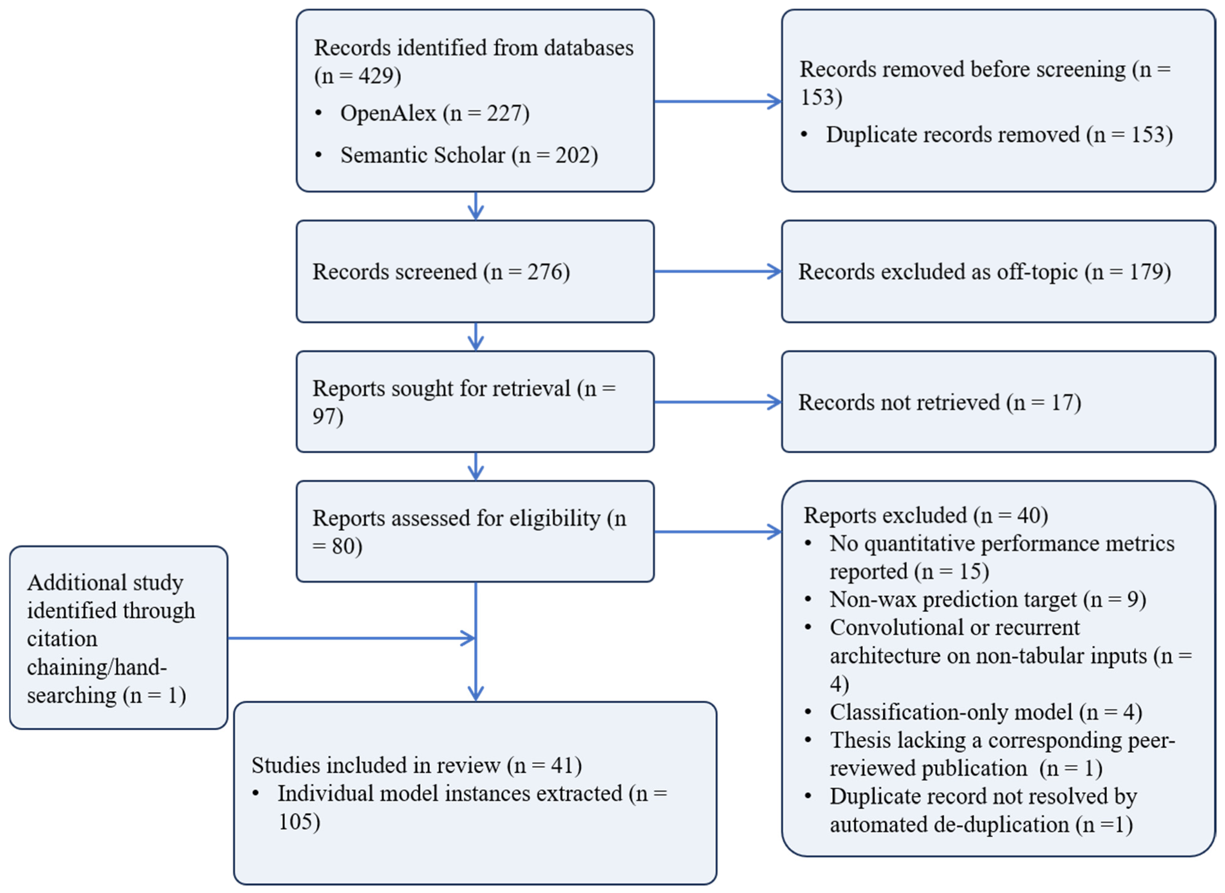
The database searches returned 429 records (227 from OpenAlex and 202 from Semantic Scholar). After the removal of 153 duplicates, 276 unique records were screened by title and abstract, of which 179 were excluded as off-topic. Of the 97 reports sought for retrieval, 17 could not be retrieved. The remaining 80 reports were assessed for eligibility in full text, and 40 were excluded with reasons: no quantitative performance metrics reported (15); non-wax-prediction target (9); non-primary/review (6); convolutional or recurrent architecture on non-tabular inputs (4); classification-only model (4); thesis lacking a corresponding peer-reviewed publication (1); and duplicate record not resolved by automated de-duplication (1). This yielded 40 studies from database searching. One further study meeting all eligibility criteria was identified through hand-searching, giving a total of 41 included studies, which together contributed 105 individual model instances to the extracted dataset. The selection process is summarized in the PRISMA 2020 flow diagram (Figure 1).

3. Data-Driven Artificial Intelligence (AI)-Based Modeling

Data-driven models learn the mapping between operational and compositional inputs and wax-related targets directly from data, without explicitly solving the underlying transport and thermodynamic equations. This section describes how such models are built (Section 2.1), how their accuracy is measured (Section 2.2), the architectures applied to wax prediction (Section 2.3), and the algorithms used to train and tune them (Section 2.4).

3.1. Model Development Workflow

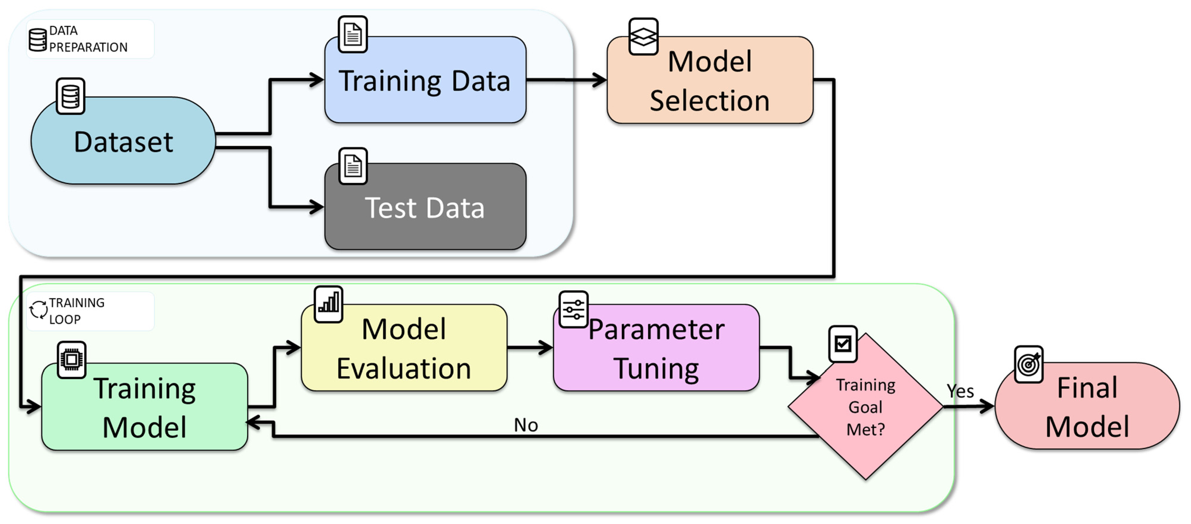
AI-based model development proceeds through five stages—data collection, preprocessing, training, validation, and optimization, as summarized in Figure 2 [28,29,30,31]. In wax prediction, the inputs are typically temperature, pressure, flow dynamics, crude oil composition (carbon-number fractions), and density, while the targets are the wax appearance temperature (WAT), wax disappearance temperature (WDT), wax deposition rate, or wax thickness (precipitated weight). Data are drawn from laboratory experiments, field measurements, process simulators (e.g., OLGA), or the compiled literature.

Preprocessing places the data on a common scale. Normalization is the most common step; it speeds convergence and prevents large-range features from dominating [29,31]. Two schemes are commonly used: min–max scaling to [0, 1] (Equation (1)), preferred for non-negative or distance-based models, and symmetric scaling to [−1, 1] (Equation (2)), preferred where zero-symmetry helps (SVM, regression, and ANN models) [32,33,34,35].

$$X_{norm}={\displaystyle \frac{X-X_{min}}{X_{max}-X_{min}}}$$

(1)

$$X_{norm}=2\cdot {\displaystyle \frac{X-X_{min}}{X_{max}-X_{min}}}-1$$

(2)

Here, $X_{norm}$ is the normalized value, $X$ is the original value, and $X_{min}$ and $X_{max}$ are the dataset minimum and maximum values.

During training, an optimization algorithm (Section 2.4) iteratively updates the model parameters to minimize the prediction error; regularization can be added to limit overfitting. Validation then evaluates the trained model on a held-out test set to confirm that it generalizes rather than memorizes: a large gap between training and test accuracy signals overfitting and prompts remedies such as reduced model complexity, more data, or cross-validation [29,31]. Finally, optimization tunes the hyperparameters of the machine learning model to balance training accuracy against generalization [36].

3.2. Evaluation Metrics

Accuracy across the reviewed literature is reported with four metrics. The coefficient of determination (R², Equation (3)) measures the explained variance, with values near 1 indicating a better fit. The mean-squared error (MSE, Equation (4)) and root-mean-squared error (RMSE, Equation (5)) measure absolute error, with lower values preferred. The average absolute percent relative error (AAPRE, Equation (6)) measures the mean relative error as a percentage. It also appears under the aliases average absolute relative deviation (AARD) and mean absolute percentage error (MAPE).

$$R^2=1-{\displaystyle \frac{{\displaystyle {\sum }_{i=1}^n}{\left(X_{pred.}^i-X_{exp.}^i\right)}^2}{{\displaystyle {\sum }_{i=1}^n}({X_{exp.}^i-{\overline{X}}_{exp})}^2}}$$

(3)

$$MSE={\displaystyle \frac{{\displaystyle {\sum }_{i=1}^n}{\left(X_{pred.}^i-X_{exp.}^i\right)}^2}{n}}$$

(4)

$$RMSE=\sqrt{{\displaystyle \frac{{\displaystyle {\sum }_{i=1}^n}{\left(X_{pred.}^i-X_{exp.}^i\right)}^2}{n}}}$$

(5)

$$AAPRE={\displaystyle \frac{100}{n}}\times {\displaystyle \sum _{i=1}^n}\left|{\displaystyle \frac{X_{exp.}^i-X_{pred.}^i}{X_{exp.}^i}}\right|$$

(6)

Here, $n$ is the number of data points; $X_{pred.}^i$ and $X_{exp.}^i$ are the $i$-th predicted and experimental values; and ${\overline{X}}_{exp}$ is the mean of the experimental values.

3.3. Model Architectures Applied for Wax Prediction

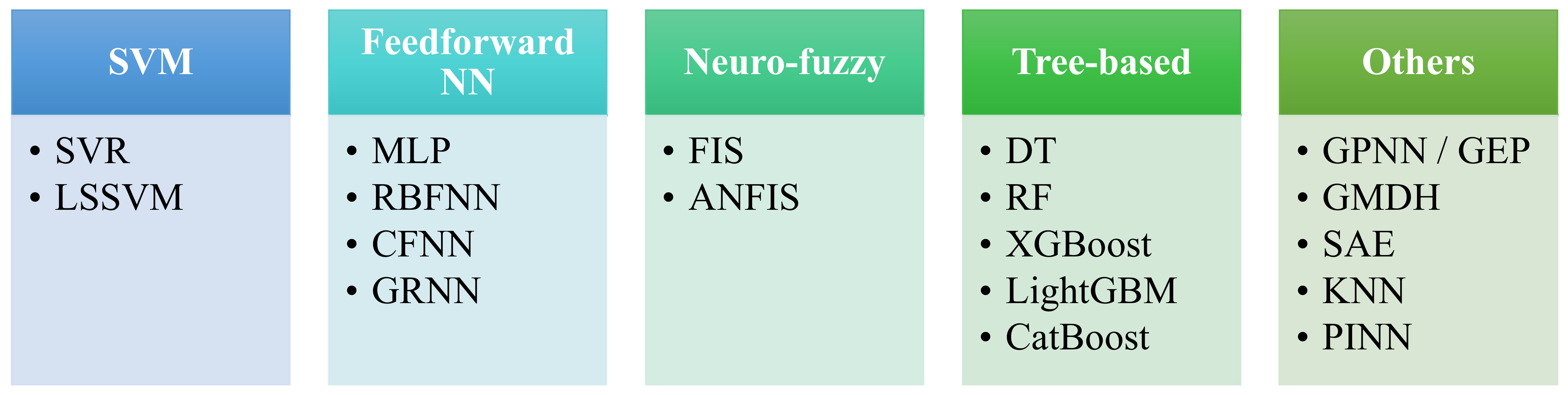
The architectures applied to wax prediction fall into five families: support vector machines (SVMs), feedforward neural networks, neuro-fuzzy systems, tree-based models, and others. Figure 3 shows this categorization. Their formulations and trade-offs are summarized in

Table 1. Architectures applied to wax deposition prediction.

Family	Model	Core Formulation/Idea	Strengths	Limitations
SVM	SVR	$y=f\left(x\right)=w\cdot \varphi \left(x\right)+b$ $\underset{w,b,\xi ,\mathit{\xi *}}{\min }{\displaystyle \frac{1}{2}}{\left|\left|w\right|\right|}^2+C\sum _{i=1}^n\left({\xi }_i+{\xi }_i^{\ast }\right)$	Robust on small noisy data; RBF kernel best	Kernel/hyperparameter sensitivity
SVM	LSSVM	$y=f\left(x\right)=w\cdot \varphi \left(x\right)+b+e_i,i=\mathrm{1,2},\dots ,n$ $\left[\begin{array}{cc}0& 1^T\\ 1& \Omega +{\displaystyle \frac{I}{\gamma }}\end{array}\right]\left[\begin{array}{c}b\\ \alpha \end{array}\right]=\left[\begin{array}{c}0\\ y\end{array}\right]$	Fast, fewer hyperparameters	Loses sparsity of SVR
Feedforward NN	MLP	$a_j^{\left(l\right)}=\mathsf{\sigma }\left({\displaystyle \sum _{i=1}^{n^{\left(l-1\right)}}}{w}_{ij}^{\left(l\right)}{a}_i^{\left(l-1\right)}+b_j^{\left(l\right)}\right)$	Universal approximator	Needs care vs. overfitting on tiny sets
	RBFNN	${\mathsf{\varphi }}_j\left(X\right)=\mathit{exp}\left(-{\displaystyle \frac{{\left|\left|X-c_j\right|\right|}^2}{2{\mathsf{\sigma }}_j^2}}\right)$	Fast local approximation	Spread/center sensitivity; scales poorly
	CFNN/GRNN	Direct skip connections/single-pass kernel regression	Quick, little/no training (GRNN)	Mostly comparison baselines
Neuro-fuzzy	FIS/ANFIS	TSK fuzzy rule: $f_i =p_i x+q_i y+r_i$	Interpretable; handles imprecision	Rule explosion with many inputs
Tree-based	DT	Recursive feature-space splits; piecewise-constant leaves	Interpretable; no feature scaling	Unstable; overfits when used alone
	RF	Bagged ensemble of de-correlated trees; outputs averaged	Robust; lowers single-tree variance	Less interpretable; weak extrapolation
	XGBoost/LightGBM/CatBoost	Gradient-boosted additive trees with regularization	Strongest on small tabular wax data	Tuning-heavy; cannot extrapolate
Others	GPNN/GEP	Genetic-programming search over network/expression structure	Evolves model structure automatically	Computationally costly; stochastic results
	GMDH	Self-organizing polynomial network; layer-wise node selection	Explicit equations; automatic structure	Polynomial term growth; overfitting risk
	KNN	Instance-based prediction from the k nearest samples using a distance metric	Simple; non-parametric; captures local nonlinear trends	Sensitive to feature scaling and choice of k; weak extrapolation
	SAE	Unsupervised layer-wise pretraining + supervised fine-tuning	Learns features from large datasets	Data-hungry; needs large sets
	PINN	Embeds governing physics as a loss regularizer	Aids extrapolation; physically consistent	Prior–data balance can bias the fit

Note. Throughout, subscripts index individual neurons, basis functions, or fuzzy rules; a superscript (l) denotes the l-th network layer; and a superscript T denotes the transpose. Symbols: x, input feature vector; X, input vector (RBFNN); y, model output (target); f(x), prediction function; w, weight vector; b, bias term; φ(·), nonlinear feature-space (kernel) mapping; ξ and ξ*, slack variables of the ε-insensitive loss; C, SVR penalty parameter; e, LSSVM regression error; γ, LSSVM regularization parameter; Ω, kernel (Gram) matrix; I, identity matrix; 1, column vector of ones; α, support-value (Lagrange-multiplier) vector; a, neuron activation; σ(·), activation function; n, number of neurons in a layer; c, basis function center; σ (subscripted), basis function width; p, q and r, consequent parameters of a Takagi–Sugeno rule; ‖·‖, Euclidean norm. Abbreviations: SVM, support vector machine; SVR, support vector regression; LSSVM, least-squares support vector machine; MLP, multilayer perceptron; RBF, radial basis function; RBFNN, radial basis function neural network; CFNN, cascade-forward neural network; GRNN, generalized regression neural network; FIS, fuzzy inference system; ANFIS, adaptive neuro-fuzzy inference system; DT, decision tree; RF, random forest; XGBoost, extreme gradient boosting; LightGBM, light gradient-boosting machine; CatBoost: Categorical Boosting; GPNN, genetic-programming neural network; GEP, gene expression programming; GMDH, group method of data handling; KNN: K-nearest neighbors; SAE, stacked auto-encoder; PINN, physics-informed neural network; NAS, neural architecture search; SHAP, Shapley additive explanations; UQ, uncertainty quantification.

.

SVMs fit a function within an ε-insensitive margin and use kernels to map inputs into a higher-dimensional space [37,38,39]. Support vector regression (SVR) is the regression form used for wax prediction. The least-squares SVM (LSSVM) replaces SVR’s inequality constraints with equality constraints and a squared-error term, reducing the problem to a linear system with fewer hyperparameters [40,41]. This lowers computational cost but sacrifices the sparsity of the standard SVM, since every training point contributes to the model. SVMs are common in wax work because the datasets are small and noisy, conditions under which margin-based regularization controls overfitting. The radial basis function (RBF) kernel is the best-performing kernel in the surveyed SVM/LSSVM studies.

Feedforward neural networks dominate the field. The multilayer perceptron (MLP) is the most common model. It is a universal approximator, trained by backpropagation, that handles the small-to-moderate tabular regression typical of wax data with minimal architecture search. However, it requires careful regularization and early stopping to avoid overfitting on small datasets. Radial basis function neural networks (RBFNNs) use localized Gaussian responses for fast training and good local approximation, but are sensitive to spread and center selection and scale poorly with input dimensionality. Cascade-forward neural networks (CFNNs), which add direct connections from each layer to all later layers, and generalized regression neural networks (GRNNs), which apply kernel regression without iterative training, appear mainly as comparison baselines [42,43].

Neuro-fuzzy systems encode if–then rules with fuzzy membership functions. Fuzzy inference systems (FISs) process information through degrees of membership rather than binary truth values, capturing uncertainty and imprecision [44,45]. The adaptive neuro-fuzzy inference system (ANFIS), introduced by Jang in 1993, overlays neural network learning onto a Takagi–Sugeno rule base, combining interpretability and adaptability with a rule count that grows combinatorially with input dimensions [46,47,48].

Tree-based models partition the feature space into regions and fit a simple prediction within each. The decision tree (DT) recursively splits the data through a root node, decision nodes, and leaf nodes, with each split chosen to minimize the prediction error (typically MSE) [29]. A single DT is interpretable but unstable, as small data changes can alter its structure. Ensembles overcome this by combining many trees. Random forests (RFs) and extremely randomized trees (extra-trees, ET) average de-correlated trees trained on bootstrap or randomized splits to reduce variance. Gradient-boosting methods such as XGBoost and LightGBM build trees sequentially and currently rank among the strongest performers on small tabular wax datasets, while CatBoost uses ordered boosting to improve generalization and efficiently handle categorical features.

Several architectures appear less frequently. Committee machines (CMs) combine parallel models, merging their outputs by averaging, voting, or weighting to improve robustness [31]. The group method of data handling (GMDH) is a polynomial neural network that builds explicit input–output relations through layers of polynomial nodes. Genetic-programming approaches like the genetic-programming neural network (GPNN) and gene expression programming (GEP) evolve the model structure itself, with GPNN evolving the network topology and GEP yielding explicit symbolic equations. The stacked auto-encoder (SAE) performs unsupervised, layer-wise feature pretraining and is justified mainly for large, often simulator-generated datasets. K-nearest neighbors (KNN) is a non-parametric, instance-based method that predicts an output from the values of the k most similar training samples, making its performance sensitive to feature scaling and the choice of k. The physics-informed neural network (PINN), the newest entrant, embeds governing physical relations into the loss as a regularizer. The Elman neural network (ENN) also appears sporadically.

3.4. AI-Based Model Training and Optimization Strategies

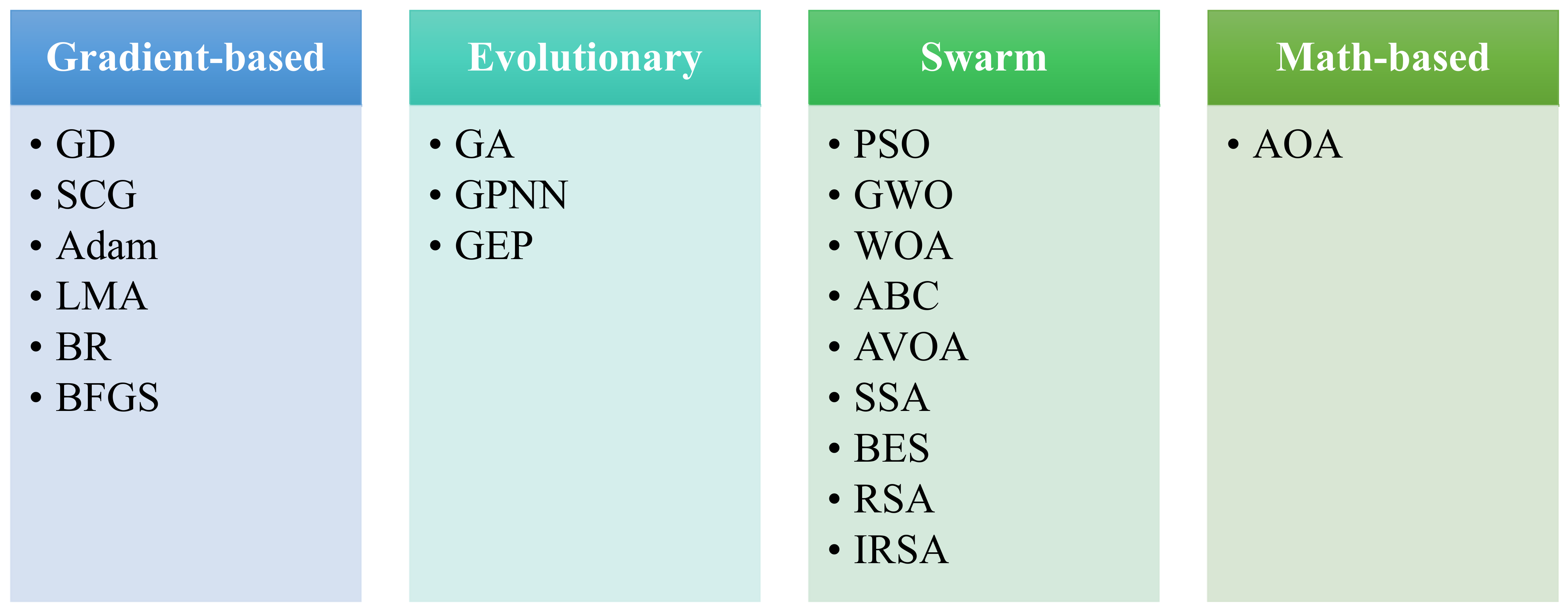
Training algorithms fall into two classes, shown in Figure 4 and detailed in

Table 2. Optimization algorithms used in wax-prediction studies.

Algorithm	Class	Core Formulation/Idea	Strengths	Role in Wax Modeling
Gradient Descent	First-order	${\mathsf{\theta }}^{\left(t+1\right)}={\mathsf{\theta }}^{\left(t\right)}-\mathsf{\eta }\nabla L\left({\mathsf{\theta }}^{\left(t\right)}\right)$	Simple, scalable	Baseline trainer
SCG	Conjugate gradient	Conjugate directions + adaptive step; auto learning rate	No line search; automatic step size	Stable; fewer hyperparameters
Adam	First-order (adaptive)	Adaptive first/second moment estimates of the gradient	Fast, robust default	Common deep-network trainer
LMA	Second-order (damped Gauss–Newton)	${\theta }^{\left(t+1\right)}={\theta }^{\left(t\right)}-{\left(J^{T}J+\mathsf{\lambda }I\right)}^{-1}{J}^{T}e$	Fast convergence on small networks	Most common MLP trainer
Bayesian Regularization	Gradient + penalty	$L\left(\mathsf{\theta }\right)=\mathsf{\alpha }{E}_D+\mathsf{\beta }{E}_W$ Weight Penalty	Auto-regularization; no separate validation set	Curbs overfitting, point estimates, not UQ
BFGS	Quasi-Newton	Iterative inverse-Hessian approximation	Superlinear convergence	Emerging; may outperform LMA
GA	Evolutionary	Selection/crossover/mutation	Global, gradient-free search	Tunes weights, architecture
GPNN	Evolutionary (GP)	Evolves network topology (NAS)	Automates network topology	Architecture search
GEP	Evolutionary (GP)	Evolves explicit expressions (genotype/phenotype split)	Yields explicit symbolic models	Symbolic model discovery
ABC	Swarm	Honeybee foraging (employed/onlooker/scout)	Few control parameters	Hybrid NN/RBFNN tuning
PSO	Swarm	Bird flock; personal + global best	Simple; fast convergence	Common ANFIS optimizer
GWO	Swarm	Gray wolf hierarchy (α/β/δ/ω)	Few parameters; good balance	Balanced exploration/exploitation
WOA	Swarm	Humpback bubble-net hunting	Simple; strong exploration	NN weight/parameter tuning
AVOA	Swarm	African vulture foraging behavior	Strong exploration; SHAP-paired	Optimizes BP NN; interpretable
AOA	Math-based	Arithmetic operators	Low-cost arithmetic operators	Optimizes Elman NN
RSA	Swarm	Reptile search	Strong exploration	Baseline for IRSA
IRSA	Swarm	Improved reptile search + chaotic map	Chaotic map improves search	Optimizes Elman NN
SSA	Swarm	Sparrow search	Fast; good convergence	Optimizes BP NN (cold-region data)
BES	Swarm	Bald eagle search (+gray relational analysis)	Balanced search; few parameters	Optimizes BP NN (diesel wax)

Note. Throughout, θ denotes the trainable parameters (network weights) and a superscript (t) is the iteration index. Symbols: η, learning rate; ∇, gradient operator; L, loss (objective) function; E_D and E_W, the data-error and weight-penalty terms of the Bayesian objective; α and β, their associated regularization hyperparameters; J, Jacobian of the residuals (Levenberg–Marquardt); λ, Levenberg–Marquardt damping parameter; I, identity matrix; e, residual (error) vector. Within the gray wolf operator, α, β, δ and ω denote the wolf-rank hierarchy rather than numerical parameters. Abbreviations: GD, gradient descent; SCG, scaled conjugate gradient; Adam, adaptive-moment estimation; LMA, Levenberg–Marquardt algorithm; BR, Bayesian regularization; BFGS, Broyden–Fletcher–Goldfarb–Shanno; GA, genetic algorithm; GP, genetic programming; GPNN, genetic-programming neural network; GEP, gene expression programming; ABC, artificial bee colony; PSO, particle swarm optimization; GWO, gray wolf optimizer; WOA, whale optimization algorithm; AVOA, African vulture optimization algorithm; AOA, arithmetic optimization algorithm; RSA, reptile search algorithm; IRSA, improved reptile search algorithm; SSA, sparrow search algorithm; BES, bald eagle search; NN, neural network; BP, backpropagation; ENN, Elman neural network; NAS, neural architecture search; SHAP, Shapley additive explanations; UQ, uncertainty quantification.

. Namely, (1) gradient-based methods, which use derivatives of the loss to descend the error surface, and (2) gradient-free metaheuristics, which search the solution space through population-based heuristics and are valuable where the objective is non-differentiable or rich in local optima.

Among the gradient-based methods, plain gradient descent and its scaled conjugate gradient (SCG) and adaptive-moment (Adam) variants are first-order schemes. The Levenberg–Marquardt algorithm (LMA) and BFGS are second-order or quasi-Newton schemes that converge faster on the small networks typical of wax models. LMA is the most common MLP trainer. Bayesian regularization (BR) adds a weight penalty to the objective to curb overfitting and is the usual benchmark against LMA.

The metaheuristics divide into evolutionary, swarm, and math-based families. Evolutionary methods (the genetic algorithm (GA), GPNN, and GEP) evolve solutions through selection, crossover, and mutation. Swarm methods, including particle swarm optimization (PSO), gray wolf optimizer (GWO), whale optimization algorithm (WOA), artificial bee colony (ABC), African vulture optimization (AVOA), sparrow search (SSA), bald eagle search (BES), and reptile search (RSA/IRSA), emulate collective animal behavior. The arithmetic optimization algorithm (AOA) is math-based. In the wax literature, these metaheuristics serve almost exclusively as weight or hyperparameter optimizers wrapped around MLP and ANFIS, with the aim of escaping local minima and avoiding manual tuning.

4. Applied AI-Based Models in Wax Deposition Prediction

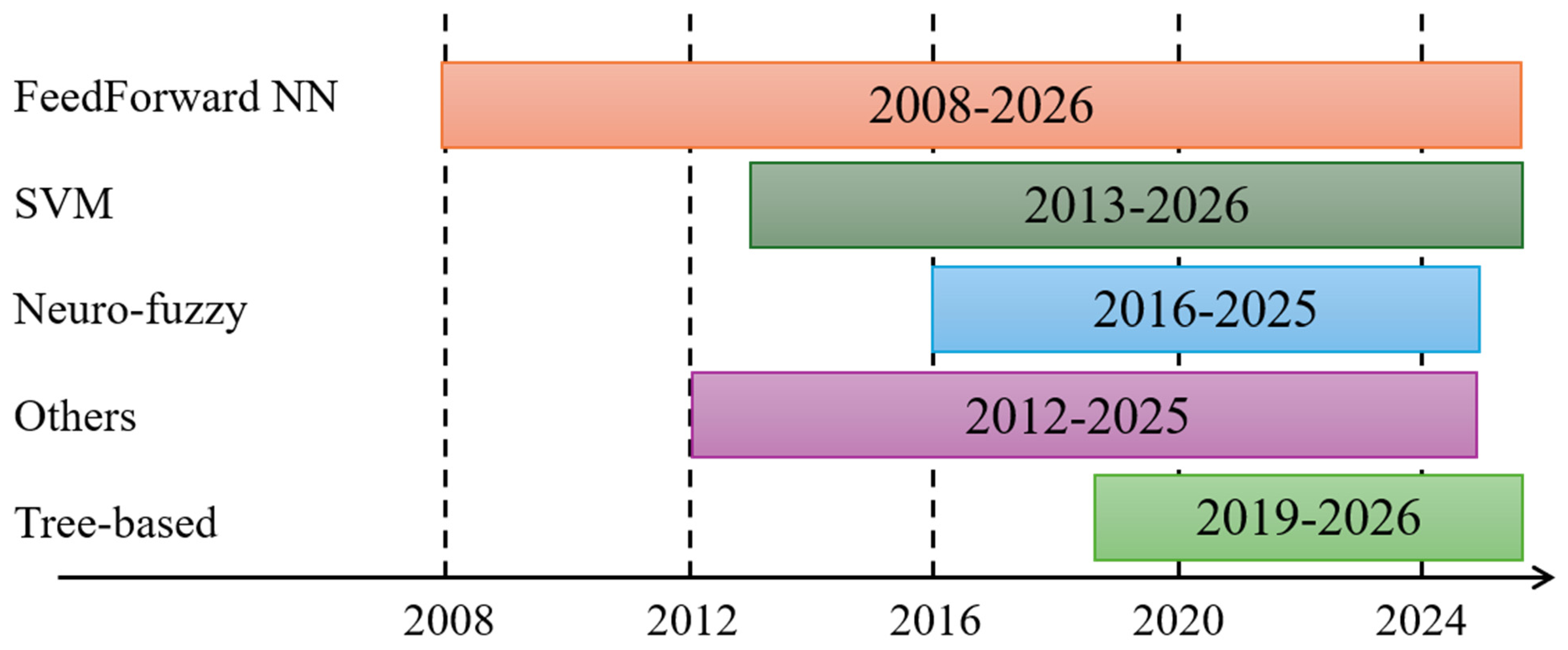
This section reviews the reported AI-based wax-prediction models, grouped by the five families of Section 2.3. Each study’s dataset, architecture, target, and test-set accuracy ($R^2$, RMSE, AAPRE) are summarized in

Table 3. Summary of SVM-based models used for wax deposition prediction (unless noted, R², AAPRE, and RMSE are test-set values).

Reference	Data Source (Size)	Input Parameters	Target	Architecture and Optimization	Summary of Results
Kamari et al. (2013) [49]	Pedersen et al. (1991) [50]; 87 pts	C1–C3, C4–C7, C8–C15, C16–C22, C23–C29, C30+, specific gravity, pressure, temperature	Wax precipitation weight	LSSVM with radial basis function kernel, C = 615.8804 and σ2 = 0.72381	R2 = 0.989 AAPRE = 36.30% RMSE = 0.440
Kamari et al. (2014) [51]	Wei et al. (2010) [52]; 10 pts	Viscosity, wall shear stress, temperature gradient at pipeline wall, wax concentration gradient	Wax deposition rate	LSSVM with radial basis function kernel, σ2 = 6.0568, γ = 13642	R2 = 0.999 AAPRE = 0.05% RMSE = 0.006
Gholami et al. (2018) [53]	Literature compilation [50,54,55]	C1–C3, C4–C7, C8–C15, C16–C22, C23–C29, C30+, specific gravity, temperature	Wax precipitation weight	SVR with sigmoid kernel function (C, ϵ, Coef, γ = 179.1758, 0.007, 0.0673, 0.1918)	R2 = 0.838 RMSE = 1.286
				SVR with radial basis function kernel, (C, ϵ, γ = 61.1818, 0.0001, 6.6548)	R2 = 0.968 RMSE = 0.570
				SVR with linear kernel function (C, ϵ = 1.3193, 0.1531)	R2 = 0.828 RMSE = 1.325
Bian et al. (2019) [56]	Literature compilation [57,58,59]; 272 pts	Pressure, molar mass	WDT	SVM-GWO with radial basis function kernel. Maximum 100 iterations, 30 search agents, (C, ϵ, γ = 35.1846, 0.0019, 0.2231)	R2 = 0.943 AAPRE = 0.69% RMSE = 2.404
				LSSVM with radial basis function kernel	R2 = 0.946 AAPRE = 0.77% RMSE = 2.824
Kamari et al. (2019) [60]	Literature compilation [57,58,59,61,62,63]; 254 pts	Pressure, molar mass	WDT	LSSVM with radial basis function kernel of C = 2138.4288 and σ2 = 40.8325	R2 = 0.950 AAPRE = 0.60% RMSE = 2.200
Septiano et al. (2022) [64]	Literature compilation [52,65,66]; 75 points, augmented to 13,995 simulated	Water volume fraction, wall shear stress, dynamic viscosity, temperature gradient at pipeline wall, wax concentration gradient	Wax deposition rate	SVR, (C,ϵ = 2.05, 0.10)	R2 = 0.945 RMSE = 0.493
Khalighi and Cheremisin (2024) [67]	Pedersen et al. (1991) [50]; 87 pts	C1–C3, C4–C7, C8–C15, C16–C22, C23–C29, C30+, Specific gravity, temperature	Wax precipitation weight	LSSVM-GA, C = 19.1668 and σ2 = 4.8490; 400 iterations, population size of 50, crossover percentage of 0.8, mutation percentage of 0.3	R2 = 0.939 RMSE = 1.113
		C4–C7, C8–C15, C16–C22, C23–C29, C30+, temperature	Wax precipitation weight	LSSVM-GA, C = 9.91e7 and σ2 = 48.8403; 400 iterations, population size of 50, crossover percentage of 0.8, mutation percentage of 0.3	R2 = 0.988 RMSE = 0.360
Kouhi et al. (2025) [68]	Literature compilation [69,70,71]; 81 pts	Density, wax content, pour point	WAT	LSSVM, with radial basis function kernel (γ = 120, σ2 = 0.2)	R2 = 0.999 AAPRE = 3.41% RMSE = 0.007
Gao et al. (2026) [72]	85 field samples, Qinghai oilfield pipeline, then augmented to 1060 via WGAN-GP	Temperature, flow velocity, wax content, pressure, viscosity	Wax deposition rate	SVR (C,ϵ,γ = 100, 0.1)	R2 = 0.961 RMSE = 0.540
Sarkodie et al. (2026) [73]	Literature compilation [66,74,75]; 215 pts	Temperature, wall temperature, viscosity, wall shear stress, flow velocity, temperature gradient at pipeline wall, wax concentration gradient	Wax deposition rate	SVR	R2 = 0.970 AAPRE = 12.32% RMSE = 0.144

,

Table 4. Summary of feedforward neural network models used for wax deposition prediction (unless noted, R², AAPRE, and RMSE are test-set values).

Reference	Data Source (Size)	Input Parameters	Target	Architecture and Optimization	Summary of Results
Huang and Ma (2008) [76]	Daqing oilfield (field); 26 pts	Viscosity, wall shear stress, temperature gradient at pipeline wall, wax concentration gradient	Wax deposition rate	MLP-LMA of shape 4-4-1	corr = 0.95
Obanijesu and Omidiora (2008) [77]	11 Nigerian crude reservoirs (field)	Viscosity	Wax deposition potential	MLP	corr = 0.970
Wei et al. (2010) [52]	Not reported	Wall shear stress, temperature gradient at pipeline wall, wax concentration gradient, viscosity	Wax deposition rate	MLP of shape 4-7-1	AAPRE < 2.00%
Manshad et al. (2012) [55]	Pedersen et al. (1991) [50]; 87 pts	C1–C3, C4–C7, C8–C15, C16–C22, C23–C29, C30+, specific gravity, pressure, temperature	Wax precipitation weight	MLP-LMA	R2 = 0.983
Kelechukwu et al. (2013) [78]	Own experiments, Malaysian crude; 360 pts	Temperature differential, flow rate, residence time	Wax deposition mass	MLP-LMA of shape 3-12-1	R2 = 0.983 (Calculated from reported data)
Moradi et al. (2013) [79]	Literature compilation [57,58,59,61,62,63]; 306 pts	Pressure, molar mass	WDT	MLP-LMA of shape 2-16-1	R2 = 0.988 AAPRE = 0.49%
Behbahani et al. (2015) [80]	Iranian waxy crude (experimental)	Temperature, oil composition, wax content	Wax precipitation/WAT	MLP-LMA of shape 3-4-10-1	AAPRE < 4.00%
Eghtedaei et al. (2017) [81]	Literature compilation [50,54,82]	C1–C3, C4–C7, C8–C15, C16–C22, C23–C29, C30+, Specific gravity, pressure, temperature	Wax precipitation weight	RBFNN-LMA	R2 = 0.998 AAPRE = 11.74% RMSE = 0.171
Saeedi Dehaghani et al. (2017) [83]	Literature compilation [84,85,86]; 1560 pts	Reynolds number, Residence time, temperature driving force, wax content	Wax deposition thickness	MLP-LM of shape 4-19-8-1	R2 = 0.999 AAPRE = 4.54%
Xie and Xing (2017) [66]	Huachi crude, from Wang 2010 [87]; 38 pts	Temperature gradient at pipeline wall, wax solubility, wall shear stress, viscosity	Wax deposition rate	RBFNN goal of 0.001 and spread of 2	AAPRE < 1.50%
Gholami et al. (2018) [53]	Literature compilation [50,54,55]	C1–C3, C4–C7, C8–C15, C16–C22, C23–C29, C30+, specific gravity, temperature	Wax precipitation weight	MLP-LMA with 6 hidden layer neurons	R2 = 0.972 MSE = 0.300 RMSE = 0.548
Benamara et al. (2019) [88]	Lit. compilation [57,58,59]; 272 pts	Pressure, molar mass	WDT	RBFNN-ABC of 36 hidden layer neurons, spread = 1.1883. Maximum of 50 iterations, 20 employer bees, 20 onlooker bees, 5 scout bees iterations.	R2 = 0.957 AAPRE = 0.61% RMSE = 2.179
				RBFNN-GA of 32 hidden layer neurons, spread = 0.5392. Maximum of 50 generations, population size of 40, crossover percentage of 0.87, mutation percentage of 0.2	R2 = 0.973 AAPRE = 0.66% RSME = 2.338
Kamari et al. (2019) [60]	Literature compilation [57,58,59,61,62,63]; 254 pts	Pressure, molar mass	WDT	MLP-LMA of shape 2-5-1	R2 = 0.950 AAPRE = 0.60% RMSE = 2.200
Mansourpoor et al. (2019) [89]	Literature compilation [57,58,62]; 310 pts	Molar mass, pressure, specific gravity	WDT	MLP-LMA of shape 3-16-1	R2 = 0.972 AAPRE = 0.38% RMSE = 1.779
Benamara et al. (2020) [90]	59 Algerian oil samples (experimental)	Density, wax tenor, pour point, freezing point, wax content	WAT	MLP-LMA of shape 5-11-10-9-1	R2 = 0.859 AAPRE = 0.74% RMSE = 2.350
				MLP-BR of shape 5-12-12-9-1	R2 = 0.907 AAPRE = 0.67% RMSE = 2.221
Amar et al. (2022) [91]	Literature compilation [50,54,55]; 88 pts	C1–C3, C4–C7, C8–C15, C16–C22, C23–C29, C30+, specific gravity, temperature	Wax precipitation weight	MLP-LMA of shape 8-11-11-9-1	R2 = 0.994 RMSE = 0.359
				MLP-BR of shape 8-11-11-9-1	R2 = 0.991 RMSE = 0.518
Askari et al. (2021) [92]	Own experimental data	Pipe size, dual-source gamma-ray detector counts	Wax deposition thickness	MLP-LMA of shape 2-18-1	RMSE = 0.040
Amiri-Ramsheh et al. (2022) [93]	Literature compilation [56,57,58,59,60,62,63,79,88]; 346 pts	Pressure, molar mass	WDT	MLP-LMA of shape 2-10-15-1	AAPRE = 0.77%, RMSE = 4.194
				MLP-BR of shape 2-10-10-1	AAPRE = 0.87%, RMSE = 4.998
				RBFNN of spread 0.1, max 65 neurons	AAPRE = 0.64%, RMSE = 2.740
Septiano et al. (2022) [64]	Literature compilation [52,65,66]; 75 points, augmented to 13,995 simulated	Water volume fraction, wall shear stress, dynamic viscosity, temperature gradient at pipeline wall, wax concentration gradient	Wax deposition rate	MLP-LMA of shape 6-56-56-1	R2 = 0.992 RMSE = 0.179
Xiao et al. (2022) [94]	Huachi oilfield [87]; 38 pts	Temperature, wall temperature, viscosity, wall shear stress, flow velocity, temperature gradient at pipeline wall, wax concentration gradient	Wax deposition rate	MLP of shape 7-7-1	R2 = 0.944 AAPRE = 8.78% RMSE = 0.894
				MLP-GA of shape 7-7-1	R2 = 0.991 AAPRE = 3.78% RMSE = 0.397
				MLP-WOA of shape 7-7-1	R2 = 0.997 AAPRE = 2.72% RMSE = 0.313
Amiri-Ramsheh et al. (2023) [95]	Literature compilation [49,96,97,98]; 173 pts	American Petroleum Institute gravity (°API), pour point	Wax precipitation weight	MLP-LMA of shape 2-10-8-1	R2 = 0.944 AAPRE = 16.59% RMSE = 1.370
				MLP-BR of shape 2-10-8-1	R2 = 0.876 AAPRE = 19.68% RMSE = 2.038
				MLP-BFGS of shape 2-10-8-1	R2 = 0.959 AAPRE = 17.18% RMSE = 1.142
				RBFNN with 90 hidden layer neurons, spread = 1.2	R2 = 0.866 AAPRE = 26.33% RMSE = 2.031
				CFNN-LMA, with 10 nodes in first and 15 nodes in second hidden layer	R2 = 0.785 AAPRE = 21.84% RMSE = 2.959
				CFNN-SCG, with 10 nodes in first and 15 nodes in second hidden layer	R2 = 0.845 AAPRE = 26.33% RMSE = 1.907
				CFNN-BFGS, with 10 nodes in first and 15 nodes in second hidden layer	R2 = 0.897 AAPRE = 21.11% RMSE = 1.757
				GRNN with spread = 0.03	R2 = 0.960 AAPRE = 10.26% RMSE = 1.113
Sultana et al. (2023) [99]	Not reported; 106 pts	Wall shear stress, viscosity, wax concentration gradient, temperature gradient at pipeline wall	Wax deposition rate	RBFNN with structure of 4-84-1 goal of 0.001 and spread of 2	R2 = 0.991 AAPRE = 1.50% RMSE = 0.860
Aguilar-Hernández et al. (2025) [100]	Experimental data; 5 samples	Pressure, paraffin content, C1–C7, C8–C15, C16–C23, C24–C30	WAT	Deep MLP, 3 hidden layers (284-1182-284), ReLU, Adam, L2, dropout, early stopping	R2 = 0.998, RMSE = 0.379 AAPRE = 9.00%,
Sarkodie et al. (2026) [73]	Literature compilation [66,74,75]; 215 pts	Temperature, wall temperature, viscosity, wall shear stress, flow velocity, temperature gradient at pipeline wall, wax concentration gradient	Wax deposition rate	MLP	R2 = 0.950 AAPRE = 15.47% RMSE = 0.185
Youcefi et al. (2026) [101]	Literature compilation [102,103,104]; 101 pts	Critical temperature of wax, temperature, pressure, critical temperature of gas system	Wax solubility	MLP-LMA of shape 4-10-8-1	R2 = 0.996 RMSE = 92.904
				MLP-BR of shape 4-10-6-1	R2 = 0.994 RMSE = 114.381,

,

Table 5. Summary of neuro-fuzzy models used for wax deposition prediction (unless noted, R², AAPRE and RMSE are test-set values).

Reference	Data Source (Size)	Input Parameters	Target	Architecture and Optimization	Summary of Results
Jalalnezhad and Kamali (2016) [105]	Literature compilation [84,85,86,106]; 1500 pts	Reynolds number, residence time, temperature driving force, wax content	Wax deposition thickness	ANFIS with range of influence of 0.23, squash factor of 0.25, accept ratio of 0.5, reject ratio of 0.15	R2 = 0.986 AAPRE = 0.01% RMSE = 0.028
Chu et al. (2017) [107]	Literature compilation [50,54,82]	C1–C3, C4–C7, C8–C15, C16–C22, C23–C29, C30+, specific gravity, pressure, temperature	Wax precipitation weight	ANFIS-PSO	R2 = 0.994 AAPRE = 21.57% RMSE = 0.290
Saeedi Dehaghani et al. (2017) [83]	Literature compilation [84,85,86]; 1560 pts	Reynolds number, residence time, temperature driving force, wax content	Wax deposition thickness	ANFIS	R2 = 0.986 AAPRE = 9.80%
Bian et al. (2019) [56]	Literature compilation [57,58,59]; 272 pts	Pressure, molar mass	WDT	ANFIS-GA	R2 = 0.870 AAPRE = 1.27% RMSE = 4.538
				ANFIS-PSO	R2 = 0.923 AAPRE = 1.34% RMSE = 5.268
Amiri-Ramsheh et al. (2022) [93]	Literature compilation [56,57,58,59,60,62,63,79,88]; 346 pts	Pressure, molar mass	WDT	ANFIS-BBO (keep rate 0.2, α 0.9, 1000 iter, pop 100)	AAPRE = 0.69%, RMSE = 3.095
				ANFIS-TLBO (1000 iter, pop 100)	AAPRE = 0.73%, RMSE = 2.945
				ANFIS-CA (accept rate 0.2, influence type 3, α = 0.9, β = 1, 1000 iter, pop 400)	AAPRE = 0.87%, RMSE = 4.672
Ahmadi (2023) [108]	Lit. compilation [50,54,82]; 88 pts	C1–C3, C4–C7, C8–C15, C16–C22, C23–C29, C30+, specific gravity, temperature	Wax precipitation weight	FIS	R2 = 0.882 RMSE = 0.136
				FIS-GA with cross-over rate of 3, 22 genes, population of 18, 125 generations, and mutation rate of 0.0075	R2 = 0.945 RMSE = 0.056
				HFGA (Hybrid of ANN, FIS and GA)	R2 = 0.968 RMSE = 0.048
Kouhi et al. (2025) [68]	Literature compilation [69,70,71]; 81 pts	Density, wax content, pour point	WAT	ANFIS	R2 = 0.966 RMSE = 2.712 AAPRE = 9.71%

,

Table 6. Summary of tree-based models used for wax deposition prediction (unless noted, R², AAPRE and RMSE are test-set values).

Reference	Data Source (Size)	Input Parameters	Target	Architecture and Optimization	Summary of Results
Kamari et al. (2019) [60]	Literature compilation [57,58,59,61,62,63]; 254 pts	Pressure, molar mass	WDT	DT	R2 = 0.970 AAPRE = 0.30% RMSE = 1.500
Amiri-Ramsheh et al. (2022) [93]	Literature compilation [56,57,58,59,60,62,63,79,88]; 346 pts	Pressure, molar mass	WDT	RF (min leaf 1, min parent 4, 250 estimators)	AAPRE = 0.29% RMSE = 1.265
				DT (min leaf 1, min parent 4.97, max split 1)	AAPRE = 0.58% RMSE = 2.570
				ET (min leaf 1, min parent 3, 10 estimators)	AAPRE = 0.53% RMSE = 2.143
Septiano et al. (2022) [64]	Literature compilation [52,65,66]; 75 points, augmented to 13,995 simulated	Water volume fraction, wall shear stress, dynamic viscosity, temperature gradient at pipeline wall, wax concentration gradient	Wax deposition rate	RF (500 estimators)	R2 = 0.993 RMSE = 0.178
Ahmadi (2025) [109]	Literature compilation [50,54,55]; 88 pts	C1–C3, C4–C7, C8–C15, C16–C22, C23–C29, C30+, specific gravity, temperature	Wax precipitation weight	XGBoost (100 trees, depth 3, learning rate: 0.1)	R2 = 0.813 RMSE = 0.339
				RF (300 trees, min samples leaf:1, min samples split:2, max depth:12)	R2 = 0.738 RMSE = 0.401
Rifat et al. (2026) [110]	Literature compilation [57,58,59,68,98,111]; 98 pts	Wax content, density, pour point	WAT	XGBoost (250 trees, learning rate: 0.05)	R2 = 0.958 AAPRE = 0.71% RMSE = 2.383
				Gradient Boosting (100 trees, learning rate: 0.05, max depth: 4)	R2 = 0.953 AAPRE = 0.67% RMSE = 2.520
				XGBoost-Gradient-Boosting Stacking Ensemble	R2 = 0.962 AAPRE = 0.67% RMSE = 2.273
				CatBoost (1000 iterations, learning rate: 0.01, depth: 4)	R2 = 0.973 AAPRE = 0.55% RMSE = 1.935
				CatBoost-GWO (800 iterations, learning rate: 0.0214, depth: 4)	R2 = 0.974 AAPRE = 0.55% RMSE = 1.882
				CatBoost-WOA (821 iterations, learning rate: 0.0119, depth: 4)	R2 = 0.973 AAPRE = 0.56% RMSE = 1.918
				CatBoost-PSO (803 iterations, learning rate: 0.0315, depth: 4)	R2 = 0.976 AAPRE = 0.51% RMSE = 1.811
Sarkodie et al. (2026) [73]	Literature compilation [66,74,75]; 215 pts	Temperature, wall temperature, viscosity, wall shear stress, flow velocity, temperature gradient at pipeline wall, wax concentration gradient	Wax deposition rate	RF	R2 = 0.998 AAPRE = 1.90% RMSE = 0.033
				Gradient Boosting	R2 = 0.985 AAPRE = 5.09% RMSE = 0.101
Yadav et al. (2026) [112]	Literature compilation [90,98,111]; 80 pts	Density, pour point, wax content	WAT	XGBoost (25 trees, max depth: 6, learning rate: 0.68)	R2 = 0.972 AAPRE = 0.69% RMSE = 2.370.
				Decision Tree (max depth: 5, min split: 2, min leaf: 2)	R2 = 0.947 AAPRE = 0.87% RMSE = 3.360
				RF (15 trees, max depth: 4, min split: 2, min leaf: 1)	R2 = 0.961 AAPRE = 0.88%, RMSE = 3.608
				ET (8 trees, max depth: 6, min split: 2, min leaf: 1)	R2 = 0.951 AAPRE = 0.77%, RMSE = 3.038
Gao et al. (2026) [72]	85 field samples, Qinghai oilfield pipeline, then augmented to 1060 via WGAN-GP	Temperature, flow velocity, wax content, pressure, viscosity	Wax deposition rate	Two-layer stacking ensemble (RF + XGBoost + SVR base; Ridge meta) + WGAN-GP augmentation	R2 = 0.963 RMSE = 0.527
				RF only (200 trees, min leaf: 5, max split: 100)	R2 = 0.937 RMSE = 0.689
				XGBoost only (200 trees, learning rate: 0.1)	R2 = 0.952 RMSE = 0.603,
Youcefi et al. (2026) [101]	Literature compilation [102,103,104]; 101 pts	Critical temperature of wax, temperature, pressure, critical temperature of gas system	Wax solubility	Extra-Trees (573 trees, max depth: 10, min samples split: 3, min leaf: 1)	R2 = 0.980 RMSE = 94.266

, and

Table 7. Summary of other AI-based models used for wax deposition prediction (unless noted, R², AAPRE, and RMSE are test-set values).

Reference	Data Source (Size)	Input Parameters	Target	Architecture and Optimization	Summary of Results
Manshad et al. (2012) [55]	Pedersen et al. (1991) [50]; 87 pts	C1–C3, C4–C7, C8–C15, C16–C22, C23–C29, C30+, specific gravity, pressure, temperature	Wax precipitation weight	GPNN	R2 = 0.931
Gholami et al. (2018) [53]	Literature compilation [50,54,55]	C1–C3, C4–C7, C8–C15, C16–C22, C23–C29, C30+, specific gravity, temperature	Wax precipitation weight	CM-GA.	R2 = 0.975 MSE = 0.250 RMSE = 0.500
Benamara et al. (2019) [88]	Lit. compilation [57,58,59]; 272 pts	Pressure, molar mass	WDT	GMDH of one input, one middle and one output layer	R2 = 0.976 AAPRE = 0.69% RMSE = 2.337
Benamara et al. (2020) [90]	59 Algerian oil samples (experimental)	Density, wax tenor, pour point, freezing point, wax content	WAT	GEP of 150 chromosomes, 11 gene, population of 420, mutation rate of 0.45, inversion rate of 0.12	R2 = 0.720 AAPRE = 1.20% RMSE = 4.398
Kim et al. (2022) [113]	OLGA simulator: 176,000 pts (2200 datasets) + 48 fine-tuning pts	Mass flow rate, inlet temperature, inlet pressure, outlet temperature, outlet pressure	Wax deposited volume, pressure, temperature of the pipeline grid	SAE, with 80 inputs and output neurons for the first training, and 5 inputs and 80 output neurons for the second training.	R2 = 0.760 (Wax volume %) R2 = 0.960 (Pressure) R2 = 0.880 (Temperature) R2 = 0.900 (Maximum wax volume %)
Chen et al. (2024) [114]	Yang 2015, Wang 2010 [115,116]; 73 pts	Flow velocity, temperature, wall temperature, wall shear stress, viscosity, wax solubility, temperature gradient at pipeline wall	Wax deposition rate	WOA-ENN	R2 = 0.999 AAPRE = 0.80% RMSE = 0.182 (Averaged performance of 2 datasets)
				RSA-ENN	R2 = 0.999 AAPRE = 0.54% RMSE = 0.116 (Averaged performance of 2 datasets)
				IRSA-ENN	R2 = 0.999 AAPRE = 0.33% RMSE = 0.070 (Averaged performance of 2 datasets)
Amar et al. (2024) [117]	Literature compilation [57,58,59]; 272 pts	Pressure, molar mass	WDT	GEP	R2 = 0.968 AAPRE = 0.55% RMSE = 2.063
Jin et al. (2025) [118]	Literature compilation [115,119,120]; 105 pts	Flow velocity, temperature, wall temperature, wall shear stress, viscosity, wax solubility, temperature gradient at pipeline wall	Wax deposition rate	ENN	AAPRE = 13.22% RMSE = 5.392 (Averaged performance of 3 datasets)
				AOA-ENN	AAPRE = 2.14% RMSE = 0.707 (Averaged performance of 3 datasets)
				PSO-ENN	AAPRE = 3.31% RMSE = 1.121 (Averaged performance of 3 datasets)
				GA-ENN	AAPRE = 4.43%, RMSE = 1.237 (Averaged performance of 3 datasets)
Ahmadi (2025) [109]	Literature compilation [50,54,55]; 88 pts	C1–C3, C4–C7, C8–C15, C16–C22, C23–C29, C30+, specific gravity, temperature	Wax precipitation weight	PINN	R2 = 0.807 RMSE = 0.344
Sarkodie et al. (2026) [73]	Literature compilation [66,74,75]; 215 pts	Temperature, wall temperature, viscosity, wall shear stress, flow velocity, temperature gradient at pipeline wall, wax concentration gradient	Wax deposition rate	KNN	R2 = 0.985 AAPRE = 8.16% RMSE = 0.101

, respectively. Where a study compared models from different families, its result is reported under each relevant subsection. Figure 5 traces when each family was adopted. Feedforward networks and SVMs span the entire period, neuro-fuzzy systems cluster in the mid-2010s, and tree-based models appear only in the most recent studies.

4.1. SVM-Based Models

In 2013, Kamari et al. [49] trained an LSSVM on Pedersen et al.’s 87-point dataset [50], reaching R² = 0.989 and RMSE = 0.440 (AAPRE = 36.30%). In 2014, Kamari et al. [51] applied an LSSVM tuned by coupled simulated annealing to the wax deposition rate, based on Wei et al.’s 10-point dataset [52], reporting R² = 0.999, RMSE = 0.006, and AAPRE = 0.05%. In 2018, Gholami et al. [53] compared SVR with sigmoid, RBF, and linear kernels for the wax deposition rate from several studies [50,54,55]. The RBF kernel was the best (R² = 0.968, RMSE ≈ 0.570), with the others reaching only R² ≈ 0.83. In 2019, Bian et al. [56] built SVM-GWO and LSSVM models for WDT from 272 points [57,58,59]. Both led their comparison with R² > 0.94, AAPRE < 1%, and RMSE < 3. The same year, Kamari et al. [60] predicted WDT with an LSSVM on 254 points [57,58,59,61,62,63] (R² = 0.95, AAPRE = 0.60%, RMSE = 2.20). In 2022, Septiano et al. [64] built an SVR model for the wax deposition rate, trained on 13,995 points simulated from 75 experimental measurements and reached R² = 0.945 and RMSE = 0.493. In 2024, Khalighi and Cheremisin [67] optimized an LSSVM with a GA on 88 samples [50]. By removing two low-relevance inputs (C₁–C₃ mole fraction and specific gravity), it raised the model from R² = 0.939 to R² = 0.988 (RMSE = 0.360). In 2025, Kouhi et al. [68] predicted WAT from 81 points using oil density, wax content, and pour point. When benchmarked against an RNN and ANFIS, the LSSVM was the most accurate (R² = 0.999, RMSE = 0.007, AARD = 3.41%), with pour point being the dominant input. In 2026, Sarkodie et al. [73] generated an SVR for the wax deposition rate on 215 compiled points under 5-fold cross-validation, resulting in R² = 0.970, AAPRE = 12.32%, and RMSE = 0.144. In the same year, Gao et al. [72] reported a standalone SVR (R² = 0.961) as the strongest single base learner in their stacking ensemble.

4.2. Feedforward Neural Network Models

MLP is by far the most common architecture. In 2008, Huang and Ma [76] trained a 4-4-1 MLP on 26 Daqing oilfield points for the wax deposition rate, reporting a correlation coefficient of 0.95 against field data. In the same year, Obanijesu and Omidiora [77] used an MLP to predict and classify wax deposition potential across 11 Nigerian reservoirs (Pearson r = 0.97). In 2010, Wei et al. [52] predicted a wax deposition rate with a 4-7-1 MLP (AAPRE < 2%). In 2012, Manshad et al. [55] predicted the wax deposition amount with an MLP on 87 points [50] (R² = 0.983), with C₈–C₁₅, C₁₆–C₂₂, and temperature being the most influential. In 2013, Kelechukwu et al. [78] trained a 3-12-1 MLP-LMA on 360 Malaysian crude points (R² = 0.983). In the same year, Moradi et al. [79] compared LMA, SCG, GDA, and BR training of a 2-16-1 MLP for WDT on 306 points [57,58,59,61,62,63]; LMA was best (R² = 0.988, AAPRE = 0.49%) and beat thermodynamic models under varying pressure. In 2015, Behbahani et al. [80] used a 3-4-10-1 MLP-LMA for wax precipitation and WAT on Iranian crude (AAPRE < 4%), exceeding solid-solution and multi-solid models. In 2017, Eghtedaei et al. [81] applied an RBFNN-LMA network to predict wax deposition amount, reaching R² = 0.998, AAPRE = 11.74%, and RMSE = 0.171. In the same year, Saeedi Dehaghani et al. [83] modeled a 4-19-8-1 MLP-LMA for predicting wax deposition thickness on 1560 points, resulting in R² = 0.999 and AAPRE = 4.54%. In 2018, Gholami et al. [53] reached R² = 0.972 (RMSE ≈ 0.548) with an MLP-LMA, slightly better than their SVR. In 2019, Kamari et al. [60] reported an MLP-LMA for WDT (R² = 0.95, AAPRE = 0.60%, RMSE = 2.20). In the same year, Mansourpoor et al. [89] used a 3-16-1 MLP-LMA for WDT on 310 points, reporting R² = 0.972, AAPRE = 0.38%, and RMSE = 1.78. In 2020, Benamara et al. [90] predicted WAT from 59 Algerian samples with a 5-11-10-9-1 MLP-LMA and a 5-12-12-9-1 MLP-BR; MLP-BR was better (R² = 0.907, AAPRE = 0.67%, RMSE = 2.221), with freezing and pour points being the most influential. In 2021, Askari et al. [92] coupled gamma-ray densitometry with an MLP-LMA to infer wax deposition thickness directly from backscattered photon counts (RMSE < 0.05), a sensor-based approach distinct from the thermophysical-input models. In 2022, Amar et al. [91] trained 8-11-11-9-1 MLP-LMA and MLP-BR on 88 points [50,54,55], both at R² ≈ 0.99 (RMSE ≈ 0.3–0.5). In the same year, Xiao et al. [94] optimized a 7-7-1 MLP for the wax deposition rate on 38 points; MLP-WOA (R² = 0.997, AAPRE = 2.72%, RMSE = 0.313) outperformed MLP-GA (R² = 0.991, AAPRE = 3.78%, RMSE = 0.397) and the un-optimized network (R² = 0.944, AAPRE = 8.78%, RMSE = 0.894). In the same year, Septiano et al. [64] also compared their MLP-LMA model with R² = 0.992 and RMSE = 0.179. In 2023, Amiri-Ramsheh et al. [95] compared feedforward models on 173 wax content measurements [49,96,97,98]; the 2-10-8-1 MLP-BFGS was best (R² = 0.959, RMSE = 1.142, AAPRE = 17.18%), ahead of MLP-LMA. In 2025, Aguilar-Hernández et al. [100] trained a three-hidden-layer MLP (284-1182-284, Adam) to estimate WAT from pressure, paraffin content, and lumped fractions, reaching R² = 0.998 (RMSE = 0.379, AAPRE = 9.00%), beating a single-hidden-layer MLP (R² = 0.961) and linear regression (R² = 0.920), with pressure being the most dominant predictor feature. In 2026, Sarkodie et al. [73] also compared with an MLP with performance of R² = 0.950, AAPRE = 15.47%, and RMSE = 0.185. In the same year, Youcefi et al. [101] collected 101 data points [102,103,104] to predict wax solubility in CO₂ and C₂H₆, with 2 MLPs and extra-trees. MLP-BR (R² = 0.994, RMSE = 114.381) and MLP- LM (R² = 0.996, RMSE = 92.904) perform best, ahead of the extra-trees model.

Other feedforward variants appear less often. In 2017, Xie and Xing [66] reached AAPRE < 1.5% with an RBFNN on 38 points [87]. In 2019, Benamara et al. [88] compared GA- and ABC-tuned RBFNNs for WDT on 272 points [57,58,59], with the ABC variant being slightly better. In 2022, Amiri-Ramsheh et al. [93] compiled 346 WDT points from multiple literature sources [57,58,59,62,63,79] and benchmarked feedforward, neuro-fuzzy, and tree-based families using only pressure and molar mass as inputs. Among the feedforward variants, the RBFNN (AAPRE = 0.635%, RMSE = 2.740) outperformed both MLP-LMA (AAPRE = 0.765%, RMSE = 4.194) and MLP-BR (AAPRE = 0.869%, RMSE = 4.998). In 2023, Sultana et al. [99] reported R² = 0.991, AAPRE = 1.50%, and RMSE = 0.860, with an RBFNN on 106 points. In the same year, Amiri-Ramsheh et al. [95] also tested RBFNN (R² = 0.866), CFNN (CFNN-BFGS best) (R² = 0.785–0.897), and GRNN (R² = 0.960), all trailing their MLPs.

4.3. Neuro-Fuzzy Models

In 2016, Jalalnezhad and Kamali [105] built an ANFIS for wax deposition thickness in turbulent flow from 1500 points [84,85,86,106] using Reynolds number, time, a dimensionless temperature driving force, and wax content (R² = 0.986, RMSE = 0.028, AAPRE = 0.10%). In 2017, Chu et al. [107] tuned an ANFIS with PSO on the literature data [50,54,82] (R² = 0.994, AAPRE = 21.57%, RMSE ≈ 0.290). In the same year, Saeedi Dehaghani et al. [83] also compared an ANFIS model, resulting in R² = 0.986 and AAPRE = 9.80%, which was outperformed by the MLP counterpart. In 2019, Bian et al. [56] found ANFIS-GA and ANFIS-PSO trailed their SVM models for WDT (R² ≈ 0.87–0.92, AAPRE = 1.2–1.3%, RMSE = 4.5–5.2). In 2022, Amiri-Ramsheh et al. [93] also tested three metaheuristic-tuned ANFIS variants: ANFIS-TLBO (AAPRE = 0.727%, RMSE = 2.945), ANFIS-BBO (AAPRE = 0.694%, RMSE = 3.095), and ANFIS-CA (AAPRE = 0.870%, RMSE = 4.672). However, these three models all trailed the tree-based models in the same study. In 2023, Ahmadi [108] proposed HFGA, a hybrid of MLP, fuzzy logic, and GA with eight inputs, which beat standalone FIS and FIS-GA on 88 points [50,54,82] (R² = 0.968, RMSE ≈ 0.048). In 2025, Kouhi et al. [68] found the ANFIS variant to be the weakest of the three architectures for WAT (R² = 0.966, RMSE = 2.712, AAPRE = 9.71%).

4.4. Tree-Based Models

Tree-based models are the most recent entrants and currently the strongest on small tabular wax data. In 2019, Kamari et al. [60] included a decision tree in their WDT comparison, where it outperformed their MLP-LMA and LSSVM (R² = 0.97, AAPRE = 0.30%, RMSE = 1.5). In 2022, Amiri-Ramsheh et al. [93] also compared decision trees, extra-trees, and random forests for WDT. The random forest was the best model overall (AAPRE = 0.288%, RMSE = 1.265), ahead of the decision tree (AAPRE = 0.579%, RMSE = 2.570) and extra-trees (AAPRE = 0.534%, RMSE = 2.143). Tree-based models outperformed every feedforward and neuro-fuzzy model in the same study. In the same year, Septiano et al.’s [64] random forest model achieved R² = 0.993 and RMSE = 0.178 performance, the best of their MLP-LMA, SVR, and RF models. In 2025, Ahmadi [109] compared XGBoost, random forest, and PINN on 88 samples [50,54,55] for wax deposition percentage. XGBoost (R² = 0.813, RMSE = 0.339) and random forest (R² = 0.738, RMSE = 0.401) performed better than PINN, with system temperature and the C₈–C₁₅/C₁₆–C₂₂ fractions dominant by SHAP analysis. In 2026, Rifat et al. [110] benchmarked gradient-boosting variants for WAT on 98 points, with CatBoost-PSO performing best (R² = 0.976, AAPRE = 0.51%, RMSE = 1.81). In the same year, Sarkodie et al. [73] also compared with a random forest and gradient boosting, where random forest was the best amongst all comparisons, with performance of R² = 0.998, AAPRE = 1.90%, and RMSE = 0.033. In the same year, Yadav et al. [112] compared random forest, decision trees, extra-trees, and XGBoost for WAT on 80 points [90,98,111]. XGBoost led (R² = 0.972, AAPRE = 0.69%, RMSE = 2.370), ahead of random forest (R² = 0.961, AAPRE = 0.88%, RMSE = 3.608), extra-trees (R² = 0.951, AAPRE = 0.77%, RMSE = 3.038), and decision trees (R² = 0.947, AAPRE = 0.87%, RMSE = 3.360). In the same year, Gao et al. [72] stacked random forest, XGBoost, and SVR base learners under a ridge meta-learner, trained on 1060 WGAN-GP-augmented samples from 85 Qinghai oilfield points, with XGBoost (R² = 0.952, RMSE = 0.603) as the best base learner and random forest (R² = 0.937, RMSE = 0.689) as the weakest base learner. In the same year, Youcefi et al. [101] found out that the extra-trees model (R² = 0.980, RMSE = 94.266) performs worst, behind the two MLP models.

4.5. Other Models

Several architectures appear only occasionally. In 2012, Manshad et al. [55] also tested a GPNN against their MLP (R² = 0.931). In 2018, Gholami et al. [53] combined SVR and MLP-LMA in a GA-weighted committee machine, their best model overall (R² = 0.975, RMSE ≈ 0.5). In 2019, Benamara et al. [88] built a GMDH that beat their RBFNN (R² = 0.976, AAPRE = 0.69%, RMSE = 2.337). In 2020, Benamara et al. [90] also reported a GEP model, which was comparatively weak (R² = 0.720, AAPRE = 1.20%, RMSE = 4.398). In 2022, Kim et al. [113] trained a stacked auto-encoder on 176,000 OLGA-simulated points (fine-tuned on 48 experimental points), reaching R² = 0.76 for wax %, 0.88 for temperature, 0.96 for pressure, and 0.90 for maximum wax volume. In 2024, Chen et al. [114] optimized an Elman NN with IRSA (against WOA and RSA) on 35 and 38 data groups [115,116]. All three models achieved R² of 0.999, with IRSA-ENN being the most accurate (RMSE = 0.070, AAPRE = 0.33%). In the same year, Amar et al. [117] developed a white-box GEP correlation for WDT on 272 points, reporting R² = 0.968, AAPRE = 0.55%, and RMSE = 2.06. In 2025, Jin et al. [118] applied AOA to an Elman NN across three datasets (total of 105 sets of data) [115,119,120], cutting AAPRE from ~9–19% to 1.5–2.5% and beating PSO- and GA-tuned versions. In the same year, Ahmadi [109] showed that the PINN performs similarly (R² = 0.807, RMSE = 0.344) to the tree-based models. In 2026, Sarkodie et al. [73] also trained a KNN, resulting in R² = 0.985, AAPRE = 8.16%, and RMSE = 0.101.

5. Discussion

5.1. Performance Landscape Across Model Families

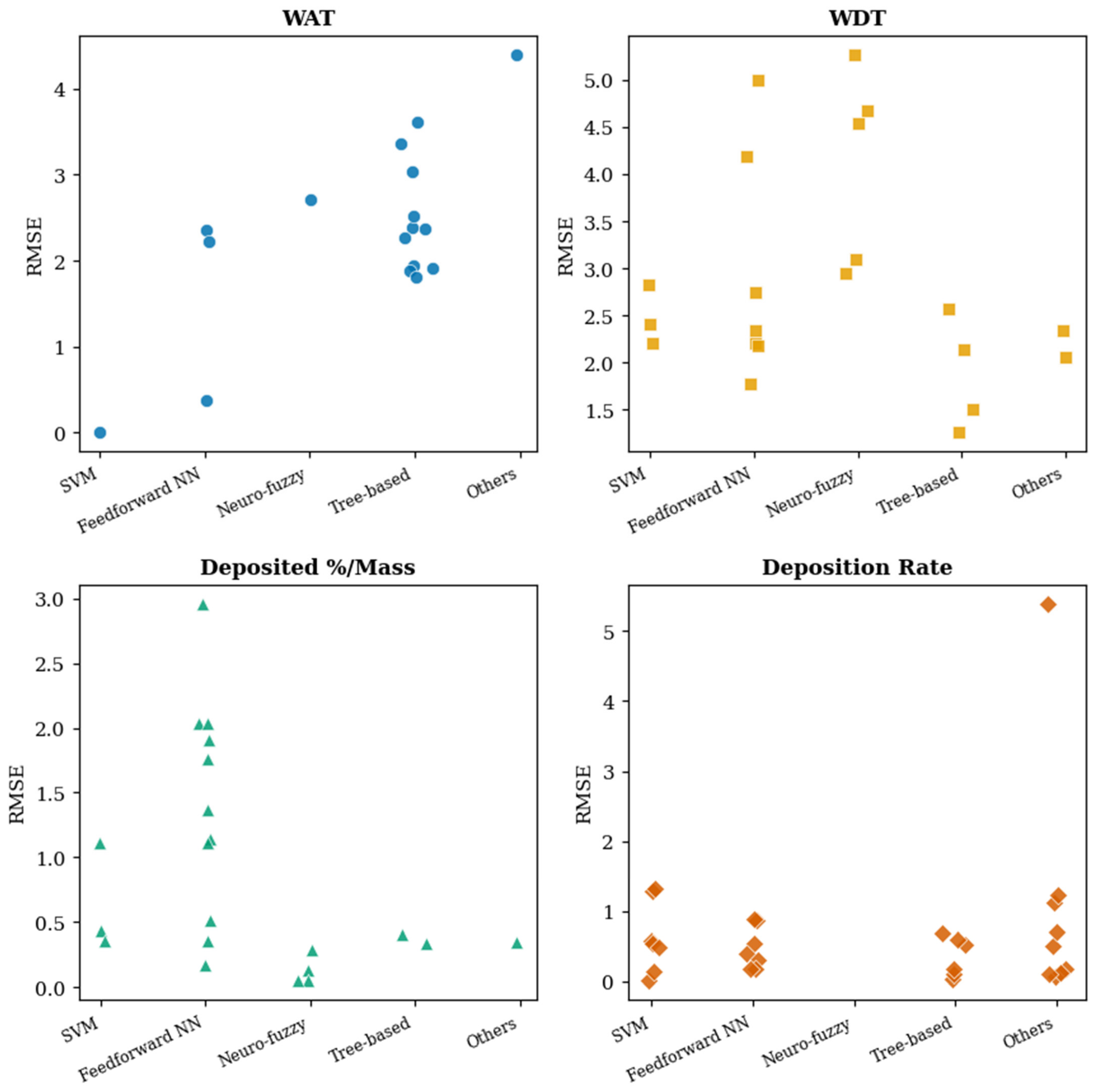
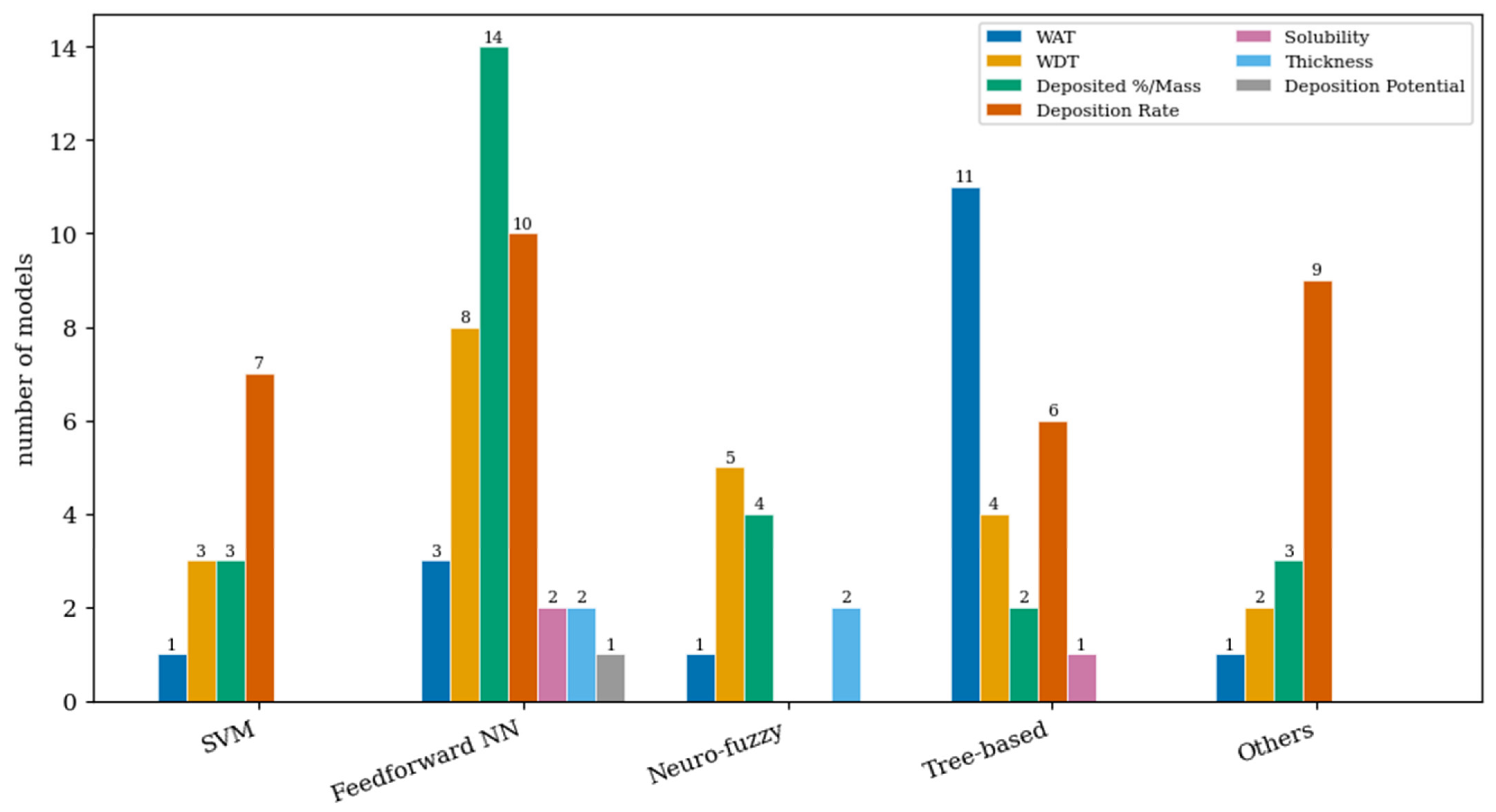
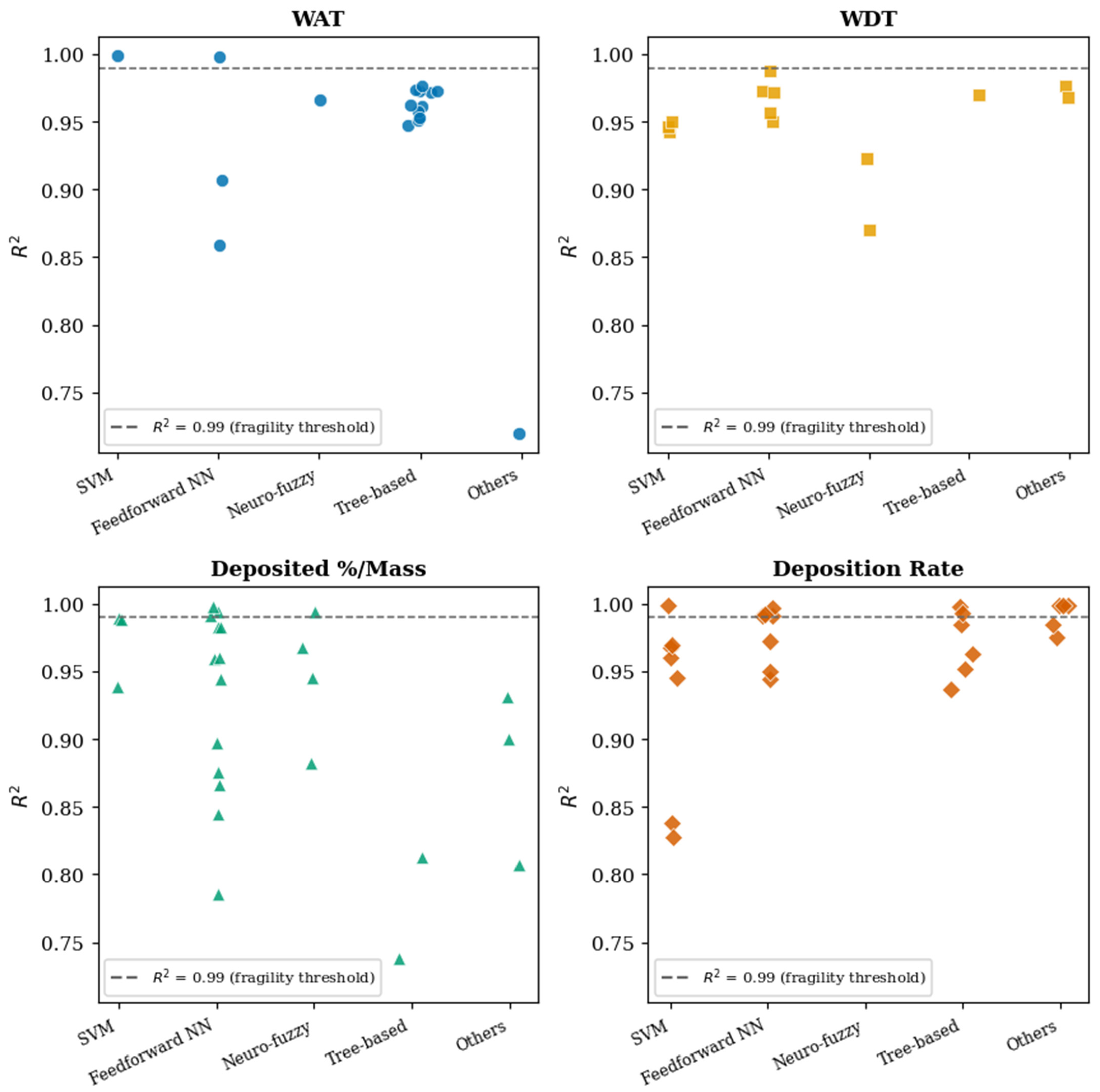
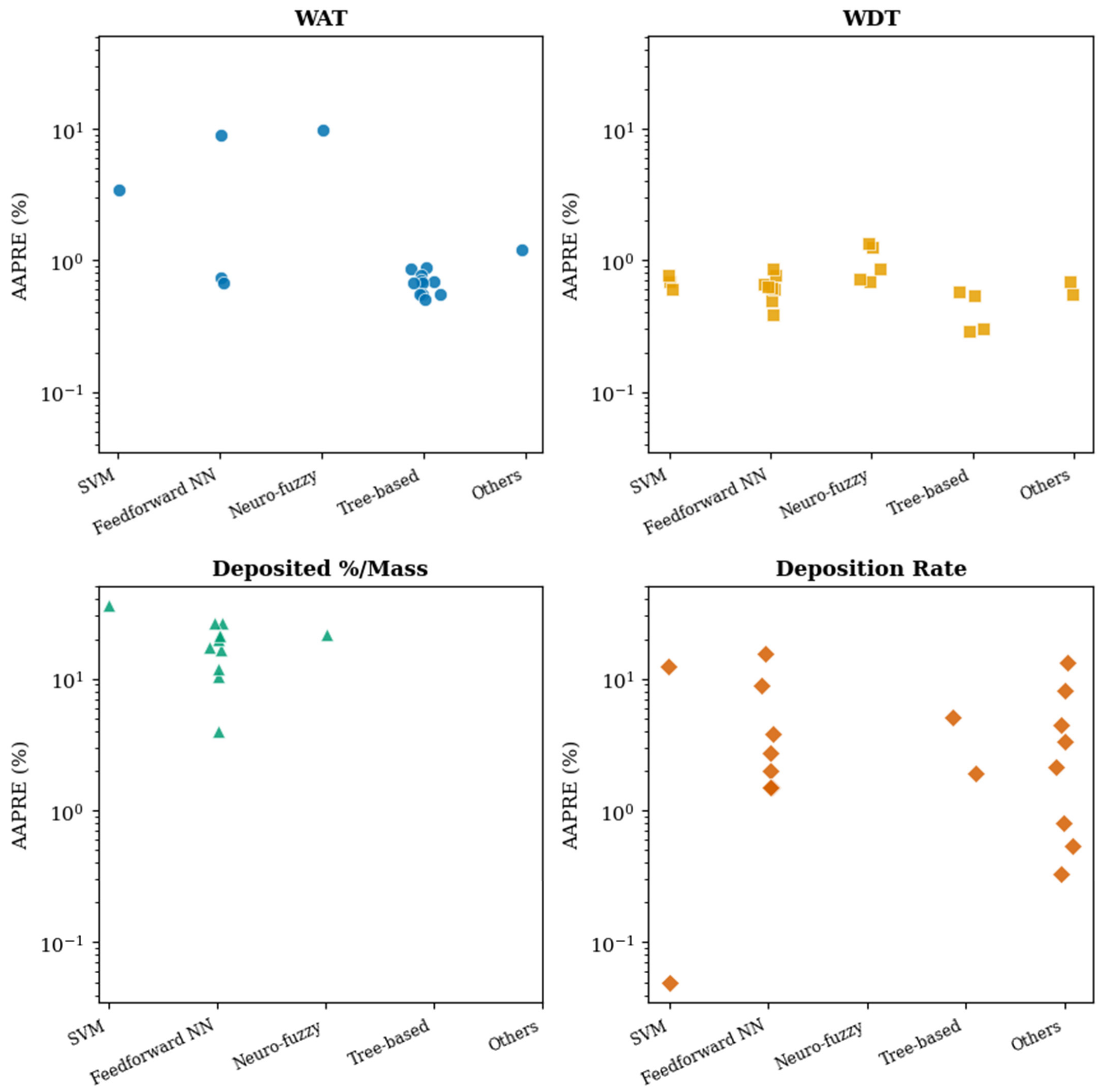
Figure 6 shows the number of models reported in each family, disaggregated by the four principal prediction targets (WAT, WDT, wax-deposited-%/mass, and wax deposition rate). The distributions of the three reported metrics are shown in Figure 7, Figure 8 and Figure 9, and the corresponding per-target summary statistics are collected in

Table 8. Per-target summary statistics of reported model performance: number of studies and models, median and interquartile range of R² and AAPRE, bootstrap 95% confidence interval of the median R², and median dataset size.

Target	Studies	Models	R2 median	R2 IQR	R2 95% CI	AAPRE Median (%)	AAPRE IQR	Median n
WAT	5	17	0.962	[0.951, 0.973]	[0.951, 0.973]	0.708	[0.668, 0.880]	80
WDT	7	22	0.957	[0.946, 0.972]	[0.946, 0.972]	0.647	[0.555, 0.756]	272
Wax Deposited % or Mass	12	26	0.944	[0.876, 0.983]	[0.882, 0.983]	20.395	[15.377, 22.962]	88
Wax Deposition Rate	12	32	0.975	[0.952, 0.993]	[0.960, 0.992]	2.72	[1.500, 6.625]	56
Wax Solubility	1	3	0.994	[0.987, 0.995]	[0.980, 0.996]
Wax Thickness	3	4	0.986	[0.986, 0.992]	[0.986, 0.999]	4.537	[2.278, 7.166]	1530
Wax Deposition Potential	1	1	0.97	[0.970, 0.970]

. Reported R² is heavily concentrated above 0.95 across all families (Figure 7). However, AAPRE (Figure 8) varies widely between targets, and RMSE (Figure 9) is scale-dependent, so it is shown per target rather than pooled.

Feedforward neural networks, and the MLP in particular, dominate the literature by volume and report consistently high accuracy, with R² frequently above 0.95 (Figure 6). For the MLP, Levenberg–Marquardt (LMA) remains the default trainer, usually benchmarked against Bayesian regularization (BR). However, no consistent winner emerges: some studies favor LMA, others BR, and Amiri-Ramsheh et al. [95] report BFGS outperforming both. This inconsistency indicates that optimizer effectiveness is dataset-dependent rather than intrinsic, so optimizer choice should be treated as a tunable hyperparameter rather than settled by convention. Among SVM models, SVR with an RBF kernel is the most accurate kernel choice [66], while LSSVM is more prevalent and routinely exceeds R² = 0.94. Neuro-fuzzy models (ANFIS) reach comparable R² but trail SVMs in direct comparison [56].

The clearest recent shift is the rise in tree-based models, most of which appeared in 2025–2026. In within-study comparisons, where models are trained and tested on identical data, gradient boosting is the most frequent winner, leading in 5 of the 13 multi-family studies and outperforming SVMs in every such comparison. However, no pairwise comparison reaches statistical significance, given the small number of head-to-head studies. The advantage is also target-dependent. For example, on the wax-weight datasets, gradient boosting is in fact the weakest family (Figure 7); XGBoost and random forest score below older feedforward networks on the same data [72,109,112]. Across studies, the median R² of tree-based models is no higher than that of established MLP or SVM work. Their real advantage is robustness on small tabular data and native interpretability through SHAP.

5.2. Dataset Scarcity and the Echo Chamber

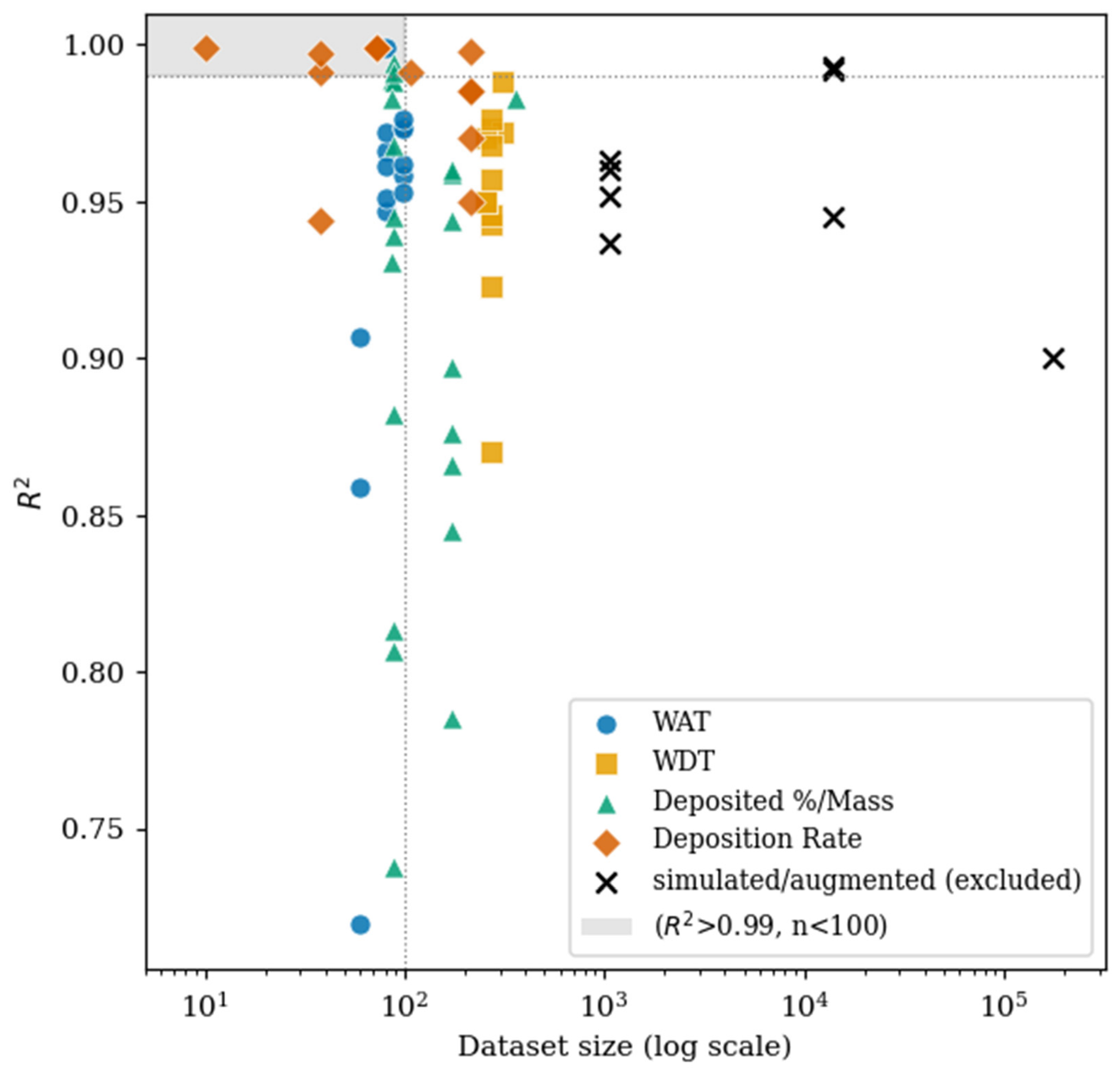
Figure 10 plots the reported R² against dataset size for every reviewed model, categorized by prediction target. Of the 87 models reporting an R², 36 achieve R² > 0.95 on fewer than 300 data points, and the median dataset across all studies is only 98 points per study once simulated, and augmented sets are excluded (mean of 244 points). Nine models attain R² > 0.99 on fewer than 100 samples (

Table 9. Models reporting R² > 0.99 on fewer than 100 data points with their source datasets.

Reference	Target	R2	n	Dataset (Source)
Kamari et al., 2014 (LSSVM) [51]	Wax Deposition Rate	0.999	10	Wei 2010 [52]
Xiao et al., 2022 (MLP-GA) [94]	Wax Deposition Rate	0.991	38	Wang 2010 [87]
Xiao et al., 2022 (MLP-WOA) [94]	Wax Deposition Rate	0.997	38	Wang 2010 [87]
Chen et al., 2024 (ENN-IRSA) [114]	Wax Deposition Rate	0.999	73	Wang 2010 [87]
Chen et al., 2024 (ENN-WOA) [114]	Wax Deposition Rate	0.999	73	Wang 2010 [87]
Chen et al., 2024 (ENN-RSA) [114]	Wax Deposition Rate	0.999	73	Wang 2010 [87]
Kouhi et al., 2025 (LSSVM) [68]	WAT	0.999	81	own WAT (81)
Amar et al., 2022 (MLP-BR) [91]	Wax Deposited % or Mass	0.991	88	Baltzer et al., Pedersen et al. compilation [50,54,55]
Amar et al., 2022 (MLP-LM) [91]	Wax Deposited % or Mass	0.994	88	Baltzer et al., Pedersen et al. compilation [50,54,55]

); for example, R² ≈ 0.999 [68] and R² ≈ 0.999 [114] on 70–90 points. Such near-perfect scores on so few samples are statistically fragile and more likely reflect in-sample fitting than genuine generalization.

Compounding this, many models draw on the same experimental datasets from the 1990s–2000s. Wax-weight studies repeatedly cite the Baltzer and Pedersen compilations [50,54,82], typically with eight or nine standard inputs (six carbon fractions C₁–C₃ … C₃₀₊, oil specific gravity, system temperature, and occasionally pressure). On the other hand, WDT studies rely on pressure and molar mass from a second recurring set (Daridon, Milhet, Ji, Metivaud and Robles [57,58,59,61,62,63]). There are 21 out of 41 studies drawn on just five shared datasets; only 16 use independent data. This creates an echo chamber effect (

Table 10. Reuse of shared source datasets across the reviewed studies.

Dataset Sources	Main Target	Studies Reusing (n)	Models (n)	Studies
Baltzer et al., Pedersen et al. compilation (1991) [50,54,55]	Wax deposited %/mass	9	20	Kamari et al., 2013 [49]; Amar et al., 2022 [91]; Ahmadi, 2023 [108]; Ahmadi, 2025 [109]; Chu et al., 2017 [107]; Manshad et al., 2012 [55]; Eghtedaei et al., 2017 [81]; Gholami et al., 2018 [53]; Khalighi and Cheremisin, 2024 [67]
Daridon et al./Milhet et al./Ji et al./Metivaud et al./Robles et al. (1995–2005) [57,58,59,61,62]	WDT	7	22	Bian et al., 2019 [56]; Kamari et al., 2019 [60]; Moradi et al., 2013 [79]; Benamara et al., 2019 [88]; Amiri-Ramsheh et al., 2022 [93]; Mansourpoor et al., 2019 [89]; Amar et al., 2024 [117]
Wang (2010) [87]	Wax deposition rate	4	11	Xie and Xing, 2017 [66]; Xiao et al., 2022 [94]; Chen et al., 2024 [114]; Jin et al., 2025 [118]
Wei et al. (2010) [52]	Wax deposition rate	3	5	Wei et al., 2010 [52]; Kamari et al., 2014 [51]; Septiano et al., 2022 [64]

), where models are repeatedly tested on near-identical data. Because the same datasets are often reused for both tuning and evaluation, agreement between studies reflects shared data rather than independent confirmation.

5.3. Comparability of Error Metrics

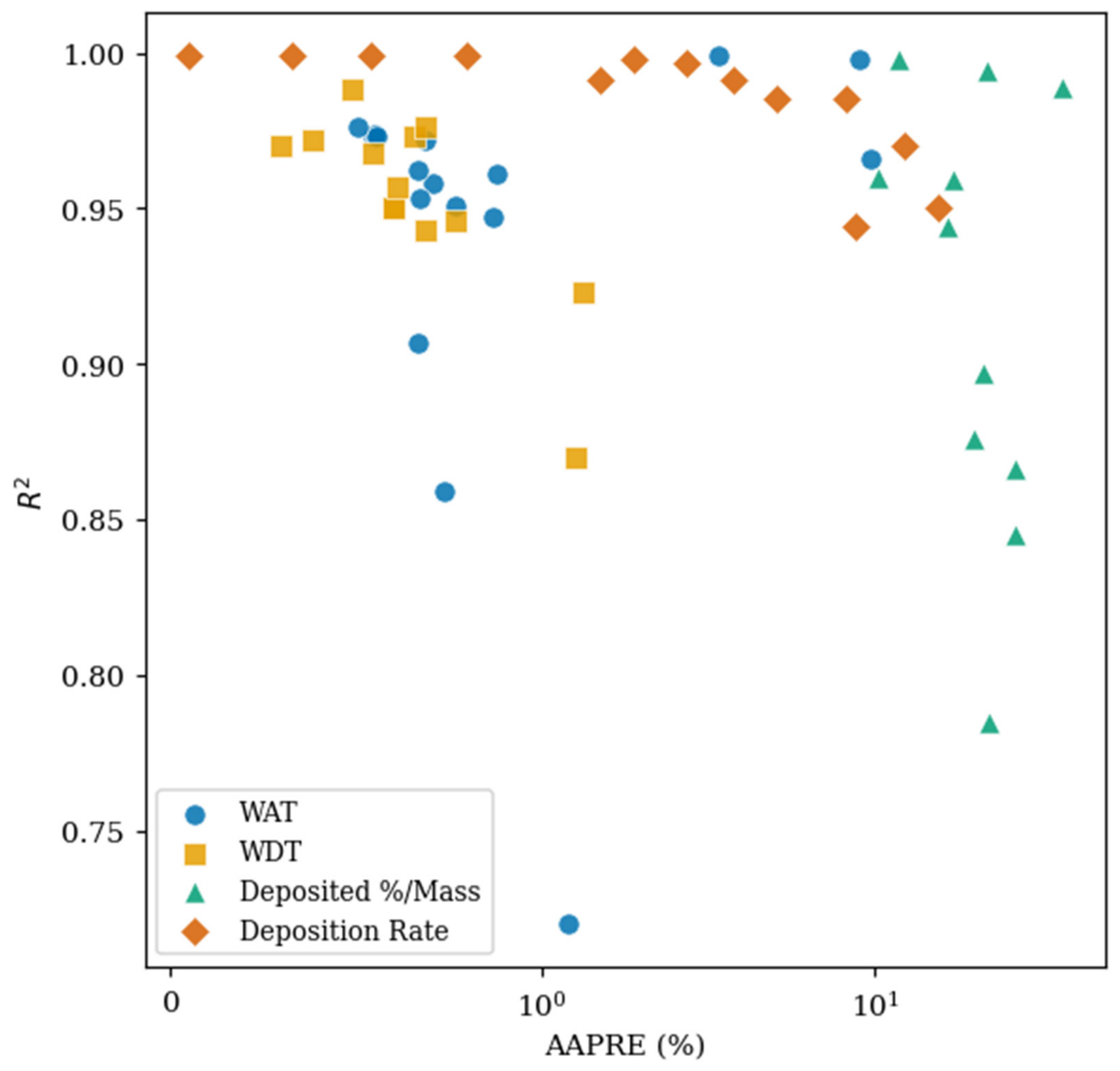
Cross-study comparison is further complicated by inconsistent, scale-dependent reporting. AAPRE is reported for only about two-thirds of the models (73 of 105). RMSE is reported more often, but it is scale-dependent (for example, <0.05 for wax thickness to 90–114 for wax solubility). As shown in Figure 9, RMSE cannot be compared across targets; hence, it is meaningful only within a single target. This leaves R² and AAPRE as the only metrics that transfer across targets. However, even these must be read together, because a high R² does not guarantee a low error.

This matters most for the wax deposited %/mass target. As shown in Figure 11, these models reach a median R² of 0.944 but a median AAPRE of about 20%. That is an order of magnitude worse than the deposition-rate target, which achieves a comparable R² at only 2.7% AAPRE. A model can therefore look excellent by R² yet be unfit for quantitative use.

The reason lies in how AAPRE is scaled. Because it is weighted inversely by the measured value (Equation (6)), the same absolute error looks very different across targets. WDT predictions (245–325 K [57,58,59,61,62,63]) show high RMSE but low AAPRE, whereas wax-weight predictions (mean ≈ 3%, range 0–13% [50,54,82]) show the reverse. R² and AAPRE are therefore the more transferable metrics, and future studies should report R², AAPRE, dataset size, and the validation protocol together.

5.4. Underused Feature Selection

Feature selection remains underutilized despite consistent evidence of its value. Khalighi and Cheremisin [67] raised R² from 0.939 to 0.988 simply by removing two low-relevance inputs (C₁–C₃ and specific gravity) using Pearson’s coefficient, identifying temperature, C₈–C_15, and C₁₆–C₂₂ as the dominant features. This is consistent with the sensitivity analysis of Manshad et al. [55] and supported by Ahmadi [108]. Xie and Xing [66] used gray relational analysis to retain viscosity, wall shear stress, temperature gradient, and the wall-wax crystal solubility coefficient. Bian et al. [56] established pressure and molar mass for WDT as the highest impact predictors, while Benamara et al. [90] and Amiri-Ramsheh et al. [95] highlighted pour and freezing points.

Therefore, systematic feature selection, such as sensitivity analysis, SHAP, mutual information, and PCA, should be performed, as they could reduce model complexity while improving interpretability and generalization [121,122].

Finally,

Table 11. A summary of the recommended AI-based models used for wax deposition prediction in this review.

Target	Input Parameters	Recommended Models
WAT	Density, viscosity, pour point, freezing point, wax content; pressure, paraffin content, lumped fractions	LSSVM [68]; deep MLP-Adam [100]; XGBoost [112]; MLP-BR [90]; CatBoost-PSO [110]
WDT	Pressure, molar mass [57,58,59,61,62,63]	LSSVM or SVM-GWO [56,60]; MLP-LMA [60,105]; RBFNN-GA or RBFNN-ABC [88]; ANFIS-PSO [56]; GMDH or DT [88]; GEP [117]
Wax deposited %/mass	C1–C3, C4–C7, C8–C15, C16–C22, C23–C29, C30+, specific gravity, temperature, pressure [50,54,82]	SVR or LSSVM or LSSVM-GA [49,53]; MLP-LMA or MLP-BR [53,55,91]; ANFIS-PSO, FIS-GA or HFGA [107,108]; CM-GA [90]; Gradient Boosting (XGBoost) emerging but lower-scoring on this target [109]; RBFNN-LMA [81]
	American Petroleum Institute Gravity (°API), pour point	MLP-LMA or MLP-BFGS [95]; GPNN [95]
	Temperature differential, flow rate, residence time	MLP-LMA [78]
Wax deposition rate	Wall shear stress, viscosity, temperature gradient at pipeline wall, wax concentration gradient	RBFNN [99]; stacked RF/XGBoost/SVR ensemble [72]; ENN-IRSA [114]; RF [73]
	Reynolds number, residual time, temperature driving force, wax content	ANFIS [105]
Wax solubility	Critical temperature of wax, temperature, pressure, critical temperature of gas system	Extra-trees or MLP-LMA [101]
Wax Thickness	Reynolds number, residence time, temperature driving force, wax content	MLP-LMA [83], ANFIS [105]

summarizes the recommended models for each prediction target.

While Table 11 provides a broad summary of the models applied to different wax-prediction targets, their reported performance cannot be directly compared because the studies frequently use different datasets, sample sizes, input variables, target scales, and validation procedures. Therefore, a more objective model-selection framework is provided in

Table 12. Model-selection guidance for AI-based wax prediction.

Prediction Target	Input Characteristics	Recommended Starting Model(s)	Justification
Wax deposited %/mass	Compositional and operating variables; small tabular datasets	MLP or LSSVM;	MLP and LSSVM are repeatedly the strongest on the shared wax-weight datasets.
Wax deposition rate	Operational/flow variables	LSSVM, RF, or gradient boosting (XGBoost/CatBoost)	CatBoost with nested/external validation [110] is the most robustly evaluated. LSSVM’s near-perfect R2 comes from a single small (n = 81) split and should be read with caution.
WDT	Pressure and molar mass	DT/RF or LSSVM	Tree models outperform NN/ANFIS alternatives in direct comparisons; LSSVM is repeatedly competitive.
WAT	Density, wax content, pour point and related variables	LSSVM or XGBoost	Best-performing models in direct within-study comparisons.
Wax solubility	Critical temperature of wax, temperature, pressure, critical temperature of gas system	MLP	MLP outperformed extra-trees in the available direct comparison.
Wax thickness	Reynolds number, residence time, temperature driving force, wax content	MLP	ANN outperformed ANFIS in the available comparison; however, evidence is limited to three studies.

. The recommendations are based on three criteria: (1) direct comparative performance, with preference given to models evaluated against alternatives using the same dataset and validation procedure; (2) consistency of competitive performance across multiple studies or datasets, where such evidence is available; and (3) suitability of the model architecture for the characteristics of the prediction problem and available data. Performance metrics obtained from different datasets or validation procedures are not used to directly rank the models.

It is worth mentioning that the practical implementation of AI-based wax deposition models depends strongly on the availability of their input variables under field operating conditions. Although laboratory datasets may contain detailed crude oil compositional information that can improve model accuracy, such information is not necessarily available at the frequency required for real-time prediction. In contrast, variables such as temperature, pressure, flow rate, viscosity, shear stress, density, pour point, and other routinely monitored process parameters can generally be obtained continuously through conventional field instrumentation and process monitoring systems. Consequently, AI models relying primarily on continuously measurable operational variables have greater potential for real-time or near-real-time implementation. Also, these parameters can partially reflect changes in the oil composition.

Therefore, the distinction between predictive accuracy and operational feasibility should be considered when evaluating AI models for field deployment. Models developed using detailed compositional information may demonstrate high accuracy on laboratory datasets but may require periodic compositional measurements rather than continuous monitoring.

A practical implementation strategy could involve a hybrid approach in which periodically obtained compositional information is used to calibrate or update the AI model, while continuously measured operational variables are used for real-time prediction.

6. Conclusions and Way Forward

This review examined artificial intelligence approaches to wax deposition prediction in oil pipelines, organizing 41 primary studies into five model families and comparing their reported accuracy on target-stratified metrics. Across the field, MLP, SVM/LSSVM, neuro-fuzzy, and, most recently, tree-based models all achieve R² values frequently above 0.95. Tree-based gradient boosting is the most frequent winner in within-study head-to-head comparisons. However, its lead is target-dependent, so no single family can be declared universally superior.

Three issues nonetheless constrain progress. First, the field depends on a small pool of recycled 1990s–2000s datasets, creating an echo chamber that inflates apparent consensus. Second, the routinely reported near-perfect accuracies are obtained on very small datasets (a median of 98 points per study) with weak validation, so they likely overstate real-world generalization. Third, inconsistent, scale-dependent metric reporting, particularly of RMSE, prevents fair cross-study comparison. A high R² can still conceal a large AAPRE error. Two secondary patterns reinforce these: (1) optimizer selection is driven by convention rather than evidence, with no consistent ranking among LMA, BR, and BFGS, and (2) systematic feature selection remains underused despite clear gains when applied.

6.1. Limitations of This Review

This review has several limitations. The systematic search relied on open bibliographic databases (OpenAlex and Semantic Scholar) supplemented by hand-searching, as subscription access to Scopus and Web of Science was unavailable. The scope was restricted to peer-reviewed, English-language primary studies, so the gray literature was excluded, and seventeen otherwise-eligible reports could not be retrieved in full text.

In addition, the performance metrics analyzed are those reported by the original authors, which could not be independently verified. Because most studies use small, frequently reused datasets and a single train–test split, these values likely represent upper bounds on true performance rather than field-realistic accuracy. Finally, metrics from different studies are not directly comparable, as they come from different datasets, units, and validation protocols. This was mitigated by analyzing each prediction target separately and by limiting performance claims to within-study or same-dataset comparisons, but some incomparability across the pooled statistics remains.

6.2. Future Directions and Recommendations

Several concrete steps would strengthen the field. First, reporting should be standardized to include R², AAPRE, dataset size, and the validation protocol together, so that studies can be compared meaningfully.

Second, validation must become more rigorous. At present, 32 of the 41 studies rely on a single train–test split, 6 add k-fold cross-validation, and only 3 use external validation on independent data, with just one (Rifat et al. [110]) applying nested cross-validation, bootstrapping, and external testing. Validation should therefore move beyond single splits toward nested cross-validation and external testing across crude types, pressure regimes, and geographies.

Third, the field needs new experimental data. Progress is currently bounded by a handful of reused legacy datasets, so generating fresh measurements across different crude types, compositions, and operating conditions is the most direct way to break the echo chamber. New studies should also evaluate their models on the established legacy datasets, so that results on new data can be benchmarked against prior work.

Fourth, practical deployability deserves explicit attention. Models intended for real-time monitoring should favor field-measurable inputs such as temperature, viscosity, shear stress, density, and pour point over full laboratory compositional analysis. Future studies should therefore evaluate AI models using field-accessible variables, quantify the effect of reducing the number of input variables on predictive performance, and validate model robustness using long-term field data. Such efforts would facilitate the transition of AI-based wax deposition models from laboratory-scale predictive tools toward real-time flow-assurance monitoring and operational decision support. Studies should also report computational cost, training time, and inference speed, which are presently almost never stated. In addition, models should quantify predictive uncertainty rather than give point estimates alone. Uncertainty quantification is almost entirely absent, yet confidence intervals are what operational decisions such as pigging scheduling actually require.

Fifth, systematic feature selection such as sensitivity analysis, SHAP, mutual information, or PCA should become routine rather than incidental.

On the modeling side, gradient-boosting ensembles paired with SHAP are the most promising near-term option for the small tabular datasets typical of this problem, combining competitive accuracy with interpretability. Physics-informed and hybrid mechanistic–data-driven models, such as PINNs, are attractive for enforcing thermodynamic consistency and improving extrapolation, provided they are evaluated on out-of-distribution conditions and against physical-trend diagnostics rather than on in-sample accuracy alone. Data-centric strategies, such as generative augmentation, simulator-generated data, and transfer learning from abundant synthetic to scarce field data, directly target the data scarcity that ultimately bounds the field. Finally, for time-resolved deposition, sequence models (LSTM and attention-based architectures) coupled to real-time sensor streams could enable online, adaptive prediction, moving wax modeling from static benchmarking toward operational flow-assurance systems. Together, these steps would move wax deposition modeling from static benchmarking on a handful of reused datasets toward reproducible, physically consistent and deployable flow-assurance tools.

References

1. Olah, G.A.; Molnár, Á. Hydrocarbon Chemistry; John Wiley & Sons: Hoboken, NJ, USA, 2003. [Google Scholar]
2. Ragunathan, T.; Husin, H.; Wood, C.D. Wax formation mechanisms, wax chemical inhibitors and factors affecting chemical inhibition. Appl. Sci. 2020, 10, 479. [Google Scholar] [CrossRef] [Scilit]
3. Srivastava, S.; Handoo, J.; Agrawal, K.; Joshi, G. Phase-transition studies in n-alkanes and petroleum-related waxes—A review. J. Phys. Chem. Solids 1993, 54, 639–670. [Google Scholar] [CrossRef] [Scilit]
4. Xie, Y.; Li, H.; Xu, M.; Su, Y.; Zhang, C.; Han, S.; Zhang, J. Effect of shear on durability of viscosity reduction of electrically-treated waxy crude oils. Energy 2023, 284, 128605. [Google Scholar] [CrossRef] [Scilit]
5. Theyab, M.A. Wax deposition process: Mechanisms, affecting factors and mitigation methods. Open Access J. Sci. 2018, 2, 112–118. [Google Scholar] [CrossRef] [Scilit]
6. Aiyejina, A.; Chakrabarti, D.P.; Pilgrim, A.; Sastry, M. Wax formation in oil pipelines: A critical review. Int. J. Multiph. Flow 2011, 37, 671–694. [Google Scholar] [CrossRef] [Scilit]
7. Zhu, H.; Lei, Y.; Yu, P.; Li, C.; Yang, F.; Yao, B.; Yang, S.; Peng, H. Wax deposition during the transportation of waxy crude oil: Mechanisms, influencing factors, modeling, and outlook. Energy Fuels 2024, 38, 9131–9152. [Google Scholar] [CrossRef] [Scilit]
8. Chen, W.; Zhang, X.; Zhao, Z.; Yin, C. UNIQUAC model for wax solution with pour point depressant. Fluid Phase Equilibria 2009, 280, 9–15. [Google Scholar] [CrossRef] [Scilit]
9. Zhang, C.; Gao, C.; Gao, F.; Wang, J.; Zhang, D.; Wang, Y.; Xu, D. Synthesis of comb bipolymers and their pour point depressing properties. Pet. Sci. 2014, 11, 155–160. [Google Scholar] [CrossRef] [Scilit]
10. Apte, M.S.; Matzain, A.; Zhang, H.-Q.; Volk, M.; Brill, J.P.; Creek, J.L. Investigation of paraffin deposition during multiphase flow in pipelines and wellbores—Part 2: Modeling. J. Energy Resour. Technol. 2001, 123, 150–157. [Google Scholar] [CrossRef] [Scilit]
11. Burger, E.; Perkins, T.; Striegler, J. Studies of wax deposition in the trans Alaska pipeline. J. Pet. Technol. 1981, 33, 1075–1086. [Google Scholar] [CrossRef] [Scilit]
12. Hernandez, O.; Hensley, H.; Sarica, C.; Brill, J.; Volk, M.; Delle-Case, E. Improvements in single-phase paraffin deposition modeling. SPE Prod. Facil. 2004, 19, 237–244. [Google Scholar] [CrossRef] [Scilit]
13. Singh, P.; Venkatesan, R.; Fogler, H.S.; Nagarajan, N. Formation and aging of incipient thin film wax-oil gels. AIChE J. 2000, 46, 1059–1074. [Google Scholar] [CrossRef] [Scilit]
14. Wang, W.; Huang, Q.; Wang, C.; Li, S.; Qu, W.; Zhao, J.; He, M. Effect of operating conditions on wax deposition in a laboratory flow loop characterized with DSC technique. J. Therm. Anal. Calorim. 2015, 119, 471–485. [Google Scholar] [CrossRef] [Scilit]
15. Sousa, A.; Matos, H.; Guerreiro, L. Preventing and removing wax deposition inside vertical wells: A review. J. Pet. Explor. Prod. Technol. 2019, 9, 2091–2107. [Google Scholar] [CrossRef] [Scilit]
16. Li, B.; Guo, Z.; Zheng, L.; Shi, E.; Qi, B. A comprehensive review of wax deposition in crude oil systems: Mechanisms, influencing factors, prediction and inhibition techniques. Fuel 2024, 357, 129676. [Google Scholar] [CrossRef] [Scilit]
17. Rittirong, A. Paraffin Deposition Under Two-Phase Gas-Oil Slug Flow in Horizontal Pipes; The University of Tulsa: Tulsa, OK, USA, 2014. [Google Scholar]
18. Rittirong, A.; Panacharoensawad, E.; Sarica, C. Experimental study of paraffin deposition under two-phase gas/oil slug flow in horizontal pipes. SPE Prod. Oper. 2017, 32, 99–117. [Google Scholar] [CrossRef] [Scilit]
19. Zhuang, Q.; Li, H.; Bao, Y.; Liu, G.; Liu, D. Research on the prediction model of wax deposition thickness of waxy crude oil in pipeline transportation. Pet. Sci. Technol. 2024, 42, 869–885. [Google Scholar] [CrossRef] [Scilit]
20. Quan, Q.; Ran, W.; Yang, L.; Gao, G.; Wang, S.; Gong, J. The effect of pressure on wax deposition from wax-solvent mixtures with natural gas. J. Pet. Sci. Eng. 2018, 171, 1318–1325. [Google Scholar] [CrossRef] [Scilit]
21. Chen, Y.; Jing, J.; Sun, J.; Wang, K.; Wang, S. Progress and perspectives of wax deposition in oil-gas systems: A review. Chem. Eng. Res. Des. 2024, 208, 348–358. [Google Scholar] [CrossRef] [Scilit]
22. Fung, G.; Backhaus, W.; McDaniel, S.; Erdogmus, M. To pig or not to pig: The marlin experience with stuck pig. In Offshore Technology Conference; OnePetro: Richardson, TX, USA, 2006; p. OTC-18387-MS. [Google Scholar]
23. Beiny, D.; Mullin, J.; Lewtas, K. Crystallization of n-dotriacontane from hydrocarbon solution with polymeric additives. J. Cryst. Growth 1990, 102, 801–806. [Google Scholar] [CrossRef] [Scilit]
24. Duan, J.; Liu, H.; Guan, J.; Hua, W.; Jiao, G.; Gong, J. Wax deposition modeling of oil/gas stratified smooth pipe flow. AIChE J. 2016, 62, 2550–2562. [Google Scholar] [CrossRef] [Scilit]
25. Ghanaei, E.; Esmaeilzadeh, F.; Fathikalajahi, J. Wax formation from paraffinic mixtures: A simplified thermodynamic model based on sensitivity analysis together with a new modified predictive UNIQUAC. Fuel 2012, 99, 235–244. [Google Scholar] [CrossRef] [Scilit]
26. Lei, Y.; Wang, H.; Li, S.-S.; Liu, X.-Q.; Zhu, H.-R.; Gao, Y.-M.; Peng, H.-P.; Yu, P.-F. Effect of existence state of asphaltenes on the asphaltenes-wax interaction in wax deposition. Pet. Sci. 2023, 20, 507–514. [Google Scholar] [CrossRef] [Scilit]
27. Yan, M.; Li, G.; Li, X. Study on the effect of crude oil composition on waxing characteristics of waxy crude oil. IOP Conf. Ser. Mater. Sci. Eng. 2018, 452, 032018. [Google Scholar] [CrossRef] [Scilit]
28. Baashar, Y.; Hamed, Y.; Alkawsi, G.; Capretz, L.F.; Alhussian, H.; Alwadain, A.; Al-Amri, R. Evaluation of postgraduate academic performance using artificial intelligence models. Alex. Eng. J. 2022, 61, 9867–9878. [Google Scholar] [CrossRef] [Scilit]
29. Géron, A. Hands-on Machine Learning with Scikit-Learn, Keras, and TensorFlow; O’Reilly Media, Inc.: Sebastopol, CA, USA, 2022. [Google Scholar]
30. Hamed, Y.; Abd Rahman, M.S.; Ab Kadir, M.Z.A.; Osman, M.; Ariffin, A.M.; Ab Aziz, N.F. Artificial intelligence forecasting for transmission line ampacity. In Towards Intelligent Systems Modeling and Simulation: With Applications to Energy, Epidemiology and Risk Assessment; Springer: Berlin/Heidelberg, Germany, 2021; pp. 217–234. [Google Scholar]
31. Haykin, S. Neural Networks and Learning Machines, 3/E; Pearson Education India: Bengaluru, India, 2009. [Google Scholar]
32. Ahsan, M.M.; Mahmud, M.P.; Saha, P.K.; Gupta, K.D.; Siddique, Z. Effect of data scaling methods on machine learning algorithms and model performance. Technologies 2021, 9, 52. [Google Scholar] [CrossRef] [Scilit]
33. Guido, R.; Ferrisi, S.; Lofaro, D.; Conforti, D. An overview on the advancements of support vector machine models in healthcare applications: A review. Information 2024, 15, 235. [Google Scholar] [CrossRef] [Scilit]
34. Rivas-Perea, P.; Cota-Ruiz, J.; Chaparro, D.G.; Venzor, J.A.P.; Carreón, A.Q.; Rosiles, J.G. Support vector machines for regression: A succinct review of large-scale and linear programming formulations. Int. J. Intell. Sci. 2013, 3, 5–14. [Google Scholar]
35. Yu, J.; Spiliopoulos, K. Normalization effects on deep neural networks. arXiv 2022, arXiv:2209.01018. [Google Scholar]
36. Yu, T.; Zhu, H. Hyper-parameter optimization: A review of algorithms and applications. arXiv 2020, arXiv:2003.05689. [Google Scholar]
37. Cortes, C.; Vapnik, V. Support-vector networks. Mach. Learn. 1995, 20, 273–297. [Google Scholar] [CrossRef] [Scilit]
38. Vapnik, V. The Nature of Statistical Learning Theory; Springer Science & Business Media: Berlin/Heidelberg, Germany, 2013. [Google Scholar]
39. Hamed, Y.; Alzahrani, A.I.; Shafie, A.F.; Mustaffa, Z.; Ismail, M.C.; Eng, K.K. Two steps hybrid calibration algorithm of support vector regression and K-nearest neighbors. Alex. Eng. J. 2020, 59, 1181–1190. [Google Scholar] [CrossRef] [Scilit]
40. Suykens, J.A.K.; Vandewalle, J. Least Squares Support Vector Machine Classifiers. Neural Process. Lett. 1999, 9, 293–300. [Google Scholar] [CrossRef] [Scilit]
41. Van Gestel, T.; De Brabanter, J.; De Moor, B.; Vandewalle, J.; Suykens, J.; Van Gestel, T. Least squares support vector machines. In Least Squares Support Vector Machines; World Scientific: Singapore, 2002; Volume 4. [Google Scholar]
42. Specht, D.F. A general regression neural network. IEEE Trans. Neural Netw. 1991, 2, 568–576. [Google Scholar] [CrossRef] [Scilit] [PubMed]
43. Warsito, B.; Santoso, R.; Suparti; Yasin, H. Cascade forward neural network for time series prediction. In Journal of Physics: Conference Series; IOP Publishing: Bristol, UK, 2018; Volume 1025, p. 012097. [Google Scholar]
44. Mamdani, E.H.; Assilian, S. An experiment in linguistic synthesis with a fuzzy logic controller. Int. J. Hum.-Comput. Stud. 1999, 51, 135–214. [Google Scholar] [CrossRef] [Scilit]
45. Zadeh, L.A. Fuzzy sets. Inf. Control 1965, 8, 338–353. [Google Scholar] [CrossRef] [Scilit]
46. Abraham, A. Adaptation of fuzzy inference system using neural learning. In Fuzzy Systems Engineering: Theory and Practice; Springer: Berlin/Heidelberg, Germany, 2005; pp. 53–83. [Google Scholar]
47. Jang, J.-S. ANFIS: Adaptive-network-based fuzzy inference system. IEEE Trans. Syst. Man. Cybern. 1993, 23, 665–685. [Google Scholar] [CrossRef] [Scilit]
48. Takagi, T.; Sugeno, M. Fuzzy identification of systems and its applications to modeling and control. IEEE Trans. Syst. Man Cybern. 1985, SMC-15, 116–132. [Google Scholar] [CrossRef] [Scilit]
49. Kamari, A.; Khaksar-Manshad, A.; Gharagheizi, F.; Mohammadi, A.H.; Ashoori, S. A Robust Model for Determination of Wax Deposition in Oil Systems. Ind. Eng. Chem. Res. 2013, 52, 15664–15672. [Google Scholar] [CrossRef] [Scilit]
50. Pedersen, W.B.; Baltzer Hansen, A.; Larsen, E.; Nielsen, A.B.; Roenningsen, H.P. Wax precipitation from North Sea crude oils. 2. Solid-phase content as function of temperature determined by pulsed NMR. Energy Fuels 1991, 5, 908–913. [Google Scholar] [CrossRef] [Scilit]
51. Kamari, A.; Mohammadi, A.H.; Bahadori, A.; Zendehboudi, S. A Reliable Model for Estimating the Wax Deposition Rate During Crude Oil Production and Processing. Pet. Sci. Technol. 2014, 32, 2837–2844. [Google Scholar] [CrossRef] [Scilit]
52. Wei, Y.; Wu, M.; Ling, Z. Wax Deposition Rate Model for Crude Oil Pipeline Based on Neural Network; IEEE: Piscataway, NJ, USA, 2010; Volume 10, pp. 760–762. [Google Scholar]
53. Gholami, A.; Ansari, H.R.; Ahmadi, S. Combining of intelligent models through committee machine for estimation of wax deposition. J. Chin. Chem. Soc. 2018, 65, 925–931. [Google Scholar] [CrossRef] [Scilit]
54. Hansen, A.B.; Larsen, E.; Pedersen, W.B.; Nielsen, A.B.; Roenningsen, H.P. Wax precipitation from North Sea crude oils. 3. Precipitation and dissolution of wax studied by differential scanning calorimetry. Energy Fuels 1991, 5, 914–923. [Google Scholar] [CrossRef] [Scilit]
55. Manshad, A.K.; Ashoori, S.; Manshad, M.K.; Omidvar, P. The prediction of wax precipitation by neural network and genetic algorithm and comparison with a multisolid model in crude oil systems. Pet. Sci. Technol. 2012, 30, 1369–1378. [Google Scholar] [CrossRef] [Scilit]
56. Bian, X.Q.; Huang, J.H.; Wang, Y.; Liu, Y.B.; Kaushika Kasthuriarachchi, D.T.; Huang, L.J. Prediction of Wax Disappearance Temperature by Intelligent Models. Energy Fuels 2019, 33, 2934–2949. [Google Scholar] [CrossRef] [Scilit]
57. Ji, H.-Y.; Tohidi, B.; Danesh, A.; Todd, A.C. Wax phase equilibria: Developing a thermodynamic model using a systematic approach. Fluid Phase Equilibria 2004, 216, 201–217. [Google Scholar] [CrossRef] [Scilit]
58. Daridon, J.L.; Pauly, J.; Milhet, M. High pressure solid–liquid phase equilibria in synthetic waxes. Phys. Chem. Chem. Phys. 2002, 4, 4458–4461. [Google Scholar] [CrossRef] [Scilit]
59. Milhet, M.; Pauly, J.; Coutinho, J.A.P.; Dirand, M.; Daridon, J.L. Liquid–solid equilibria under high pressure of tetradecane+pentadecane and tetradecane+hexadecane binary systems. Fluid Phase Equilibria 2005, 235, 173–181. [Google Scholar] [CrossRef] [Scilit]
60. Kamari, A.; Rahimzadeh, A.; Mohammadi, A.H.; Ramjugernath, D. Evaluation of wax disappearance temperatures in hydrocarbon fluids using soft computing approaches. Pet. Sci. Technol. 2019, 37, 829–836. [Google Scholar] [CrossRef] [Scilit]
61. Robles, L.; Espeau, P.; Mondieig, D.; Haget, Y.; Oonk, H.A.J. Polymorphisme et alliages moleculaires dans le systeme C17H36-C19H40. Thermochim. Acta 1996, 274, 61–72. [Google Scholar] [CrossRef] [Scilit]
62. Metivaud, V.; Rajabalee, F.; Oonk, H.A.; Mondieig, D.; Haget, Y. Complete determination of the solid (RI)-liquid equilibria of four consecutive n-alkane ternary systems in the range C14H30-C21H44 using only binary data. Can. J. Chem. 1999, 77, 332–339. [Google Scholar] [CrossRef] [Scilit]
63. Vafaie-Sefti, M.; Mousavi-Dehghani, S.A.; Mohammad-Zadeh Bahar, M. Modification of multisolid phase model for prediction of wax precipitation: A new and effective solution method. Fluid Phase Equilibria 2000, 173, 65–80. [Google Scholar] [CrossRef] [Scilit]
64. Septiano, J.; Yasutra, A.; Rahmawati, S.D. Build of Machine Learning Proxy Model for Prediction of Wax Deposition Rate in Two Phase Flow Water-Oil. Sci. Contrib. Oil Gas. 2022, 45, 53–67. [Google Scholar] [CrossRef] [Scilit]
65. Fan, K.; Huang, Q.; Li, S.; Yu, W. The wax deposition rate of water-in-crude oil emulsions based on the laboratory flow loop experiment. J. Dispers. Sci. Technol. 2017, 38, 8–18. [Google Scholar] [CrossRef] [Scilit]
66. Xie, Y.; Xing, Y. A prediction method for the wax deposition rate based on a radial basis function neural network. Petroleum 2017, 3, 237–241. [Google Scholar] [CrossRef] [Scilit]
67. Khalighi, J.; Cheremisin, A. Wax precipitation prediction using a novel intelligent method: Modeling and data analysis. Pet. Sci. Technol. 2024, 42, 846–868. [Google Scholar]
68. Kouhi, M.M.; Shafiei, A.; Bekkuzhina, T.; Abutalip, M. New intelligent models for predicting wax appearance temperature using experimental data–Flow assurance implications. Fuel 2025, 380, 133146. [Google Scholar] [CrossRef] [Scilit]
69. Zhang, Y.; Gong, J.; Wu, H. An Experimental Study on Wax Deposition of Water in Waxy Crude Oil Emulsions. Pet. Sci. Technol. 2010, 28, 1653–1664. [Google Scholar] [CrossRef] [Scilit]
70. Hoffmann, R.; Amundsen, L. Single-Phase Wax Deposition Experiments. Energy Fuels 2009, 24, 1069–1080. [Google Scholar] [CrossRef] [Scilit]
71. Quan, Q.; Gong, J.; Wang, W.; Wang, P. The Influence of Operating Temperatures on Wax Deposition During Cold Flow and Hot Flow of Crude Oil. Pet. Sci. Technol. 2015, 33, 272–277. [Google Scholar] [CrossRef] [Scilit]
72. Gao, Y.; Luo, Z.; Guo, J. A WGAN-GP and stacking ensemble-based framework for enhanced prediction of wax deposition rate in crude oil pipelines. Sci. Rep. 2026, 16, 19989. [Google Scholar] [CrossRef] [Scilit] [PubMed]
73. Sarkodie, K.; Agyepong, J.; Agyei, E.; Arkoh, G.; Arhin, R.; Ankomah, F.; Adenutsi, C.D.; Erzuah, S. Machine learning-based surrogate correlation for prediction of wax deposition rate in oil and gas pipelines. Petroleum 2026, 12, 350–365. [Google Scholar] [CrossRef] [Scilit]
74. Wang, W.; Huang, Q. Prediction for wax deposition in oil pipelines validated by field pigging. J. Energy Inst. 2014, 87, 196–207. [Google Scholar] [CrossRef] [Scilit]
75. Yao, B.; Zhao, D.; Zhang, Z.; Huang, C. Safety study on wax deposition in crude oil pipeline. Processes 2021, 9, 1572. [Google Scholar] [CrossRef] [Scilit]
76. Huang, Q.; Ma, J. Prediction of wax deposition of crude using statistical and neural network methods. In International Pipeline Conference; ASME: New York, NY, USA, 2008; Volume 48609, pp. 341–345. [Google Scholar]
77. Obanijesu, E.O.; Omidiora, E.O. Artificial neural network’s prediction of wax deposition potential of Nigerian crude oil for pipeline safety. Pet. Sci. Technol. 2008, 26, 1977–1991. [Google Scholar] [CrossRef] [Scilit]
78. Kelechukwu, E.M.; Al-Salim, H.S.; Saadi, A. Prediction of wax deposition problems of hydrocarbon production system. J. Pet. Sci. Eng. 2013, 108, 128–136. [Google Scholar] [CrossRef] [Scilit]
79. Moradi, G.; Mohadesi, M.; Moradi, M.R. Prediction of wax disappearance temperature using artificial neural networks. Pet. Sci. Eng. 2013, 108, 74–81. [Google Scholar] [CrossRef] [Scilit]
80. Behbahani, T.J.; Beigi, A.A.M.; Taheri, Z.; Ghanbari, B. Investigation of wax precipitation in crude oil: Experimental and modeling. Petroleum 2015, 1, 223–230. [Google Scholar] [CrossRef] [Scilit]
81. Eghtedaei, R.; Sasanipour, J.; Zarrabi, H.; Palizian, M.; Baghban, A. Estimation of wax deposition in the oil production units using RBF-ANN strategy. Pet. Sci. Technol. 2017, 35, 1737–1742. [Google Scholar] [CrossRef] [Scilit]
82. Pedersen, K.S.; Skovborg, P.; Roenningsen, H.P. Wax precipitation from North Sea crude oils. 4. Thermodynamic modeling. Energy Fuels 1991, 5, 924–932. [Google Scholar] [CrossRef] [Scilit]
83. Saeedi Dehaghani, A.H. An intelligent model for predicting wax deposition thickness during turbulent flow of oil. Pet. Sci. Technol. 2017, 35, 1706–1711. [Google Scholar] [CrossRef] [Scilit]
84. Lund, H.J. Investigation of Paraffin Deposition During Single Phase Flow in Pipelines. Ph.D. Thesis, University of TULSA, Tulsa, OK, USA, 1998. [Google Scholar]
85. Venkatesan, R. The Deposition and Rheology of Organic Gels; The University of Michigan: Ann Arbor, MI, USA, 2004. [Google Scholar]
86. Hernandez, O.C. Investigation of Single-Phase Paraffin Deposition Characteristics. Master’s Thesis, The University of Tulsa, Tulsa, OK, USA, 2002. [Google Scholar]
87. Wang, X.L. The Wax Deposition Phenomena Prediction of Huachi Oil Pipelines; Xi’an Shiyou University: Xi’an, China, 2010. [Google Scholar]
88. Benamara, C.; Nait Amar, M.; Gharbi, K.; Hamada, B. Modeling Wax Disappearance Temperature Using Advanced Intelligent Frameworks. Energy Fuels 2019, 33, 10959–10968. [Google Scholar] [CrossRef] [Scilit]
89. Mansourpoor, M.; Azin, R.; Osfouri, S.; Izadpanah, A. Experimental measurement and modeling study for estimation of wax disappearance temperature. J. Dispers. Sci. Technol. 2019, 40, 161–170. [Google Scholar] [CrossRef] [Scilit]
90. Benamara, C.; Gharbi, K.; Nait Amar, M.; Hamada, B. Prediction of Wax Appearance Temperature Using Artificial Intelligent Techniques. Arab. J. Sci. Eng. 2020, 45, 1319–1330. [Google Scholar] [CrossRef] [Scilit]
91. Amar, M.N.; Jahanbani Ghahfarokhi, A.; Shang Wui Ng, C. Predicting wax deposition using robust machine learning techniques. Petroleum 2022, 8, 167–173. [Google Scholar] [CrossRef] [Scilit]
92. Askari, M.; Taheri, A.; Kochakpour, J.; Sasanpour, M.T. An intelligent gamma-ray technique for determining wax thickness in pipelines. Appl. Radiat. Isot. 2021, 172, 109667. [Google Scholar] [CrossRef] [Scilit] [PubMed]
93. Amiri-Ramsheh, B.; Safaei-Farouji, M.; Larestani, A.; Zabihi, R.; Hemmati-Sarapardeh, A. Modeling of wax disappearance temperature (WDT) using soft computing approaches: Tree-based models and hybrid models. J. Pet. Sci. Eng. 2022, 208, 109774. [Google Scholar] [CrossRef] [Scilit]
94. Xiao, R.; Jin, S. Prediction model of wax deposition rate based on woabpnn algorithm. Front. Heat Mass Transf. 2022, 18, 1–7. [Google Scholar] [CrossRef] [Scilit]
95. Amiri-Ramsheh, B.; Zabihi, R.; Hemmati-Sarapardeh, A. Modeling wax deposition of crude oils using cascade forward and generalized regression neural networks: Application to crude oil production. Geoenergy Sci. Eng. 2023, 224, 211613. [Google Scholar] [CrossRef] [Scilit]
96. Roenningsen, H.P.; Bjoerndal, B.; Baltzer Hansen, A.; Batsberg Pedersen, W. Wax precipitation from North Sea crude oils: 1. Crystallization and dissolution temperatures, and Newtonian and non-Newtonian flow properties. Energy Fuels 1991, 5, 895–908. [Google Scholar] [CrossRef] [Scilit]
97. Lira-Galeana, C.; Firoozabadi, A.; Prausnitz, J.M. Thermodynamics of wax precipitation in petroleum mixtures. AIChE J. 1996, 42, 239–248. [Google Scholar] [CrossRef] [Scilit]
98. Elsharkawy, A.M.; Al-Sahhaf, T.A.; Fahim, M.A. Wax deposition from Middle East crudes. Fuel 2000, 79, 1047–1055. [Google Scholar] [CrossRef] [Scilit]
99. Sultana, F.; Abdallah, E.M.; Dong, S.; Mukhtar, Y.M.F. Development of Predictive Model for Wax Formation in Deep-water Pipeline Using Machine learning. In Journal of Physics: Conference Series; IOP Publishing: Bristol, UK, 2023; Volume 2594, p. 012042. [Google Scholar]
100. Aguilar-Hernández, M.; Sheremetov, L.; Ortega-Rodríguez, A. Predicting wax formation in High-Pressure conditions for condensate samples using Machine learning. Fuel 2025, 394, 135183. [Google Scholar] [CrossRef] [Scilit]
101. Youcefi, M.R.; Alatefi, S.; Nait Amar, M.; Alkouh, A. Data-driven modeling of wax solubility in supercritical carbon dioxide and ethane systems. J. Supercrit. Fluids 2026, 230, 106867. [Google Scholar] [CrossRef] [Scilit]
102. Mohammadi, A.H.; Eslamimanesh, A.; Richon, D. Wax Solubility in Gaseous System: Thermodynamic Consistency Test of Experimental Data. Ind. Eng. Chem. Res. 2011, 50, 4731–4740. [Google Scholar] [CrossRef] [Scilit]
103. Mohammadi, A.H.; Gharagheizi, F.; Eslamimanesh, A.; Richon, D. Evaluation of experimental data for wax and diamondoids solubility in gaseous systems. Chem. Eng. Sci. 2012, 81, 1–7. [Google Scholar] [CrossRef] [Scilit]
104. Kondori, J.; Hashemi, H.; Babaee, S.; Javanmardi, J.; Mohammadi, A.H.; Ramjugernath, D. A thermodynamic consistency test for experimental isobaric data of wax solubility in gaseous systems. Fluid Phase Equilibria 2015, 388, 182–187. [Google Scholar] [CrossRef] [Scilit]
105. Jalalnezhad, M.J.; Kamali, V. Development of an intelligent model for wax deposition in oil pipeline. J. Pet. Explor. Prod. Technol. 2016, 6, 129–133. [Google Scholar] [CrossRef] [Scilit]
106. Rosvold, K. Wax Deposition Models. Master’s Thesis, Norwegian University of Science and Technology, Trondheim, Norway, 2008. [Google Scholar]
107. Chu, Z.Q.; Sasanipour, J.; Saeedi, M.; Baghban, A.; Mansoori, H. Modeling of wax deposition produced in the pipelines using PSO-ANFIS approach. Pet. Sci. Technol. 2017, 35, 1974–1981. [Google Scholar] [CrossRef] [Scilit]
108. Ahmadi, M. Data-driven approaches for predicting wax deposition. Energy 2023, 265, 126296. [Google Scholar] [CrossRef] [Scilit]
109. Ahmadi, M. From composition to deposition: A machine learning framework for wax deposition prediction in petroleum fluids using compositional properties. Phys. Fluids 2025, 37, 072132. [Google Scholar] [CrossRef] [Scilit]
110. Rifat, H.R.; Abduljabbar, A.; Mohyaldinna, M.E. Categorical Boosting-PSO: A SHAP-Interpretable Hybrid Framework for High-Fidelity Wax Appearance Temperature Prediction in Subsea Pipelines. Eng. Rep. 2026, 8, e70979. [Google Scholar] [CrossRef] [Scilit]
111. Alcazar-Vara, L.A.; Buenrostro-Gonzalez, E. Characterization of the wax precipitation in Mexican crude oils. Fuel Process. Technol. 2011, 92, 2366–2374. [Google Scholar] [CrossRef] [Scilit]
112. Yadav, A.; Karamti, H.; Sur, D.; Menon, S.V.; Issa, B.S.; Shit, D.; Sunitha, S.; Panigrahi, R. Toward accurate modeling of wax appearance temperature (WAT) using intelligent ensemble techniques: Application to heavy crude oil production. Chem. Eng. Sci. 2025, 319, 122296. [Google Scholar] [CrossRef] [Scilit]
113. Kim, J.H.; Han, S.L.; Seo, Y.J.; Moon, B.; Lee, Y.S. The development of an AI-based model to predict the location and amount of wax in oil pipelines. J. Pet. Sci. Eng. 2022, 209, 109813. [Google Scholar] [CrossRef] [Scilit]
114. Chen, Z.; Wang, N.; Jin, W.; Li, D. Prediction Model of Wax Deposition Rate in Waxy Crude Oil Pipelines by Elman Neural Network Based on Improved Reptile Search Algorithm. Energy Eng. 2024, 121, 1007–1026. [Google Scholar] [CrossRef] [Scilit]
115. Wang, X.L. Prediction and Analysis of Wax Deposition in Pipeline Crude Oil in Huachi Operation Area. Master’s Thesis, Xi’an Shiyou University, Xi’an, China, 2010. [Google Scholar]
116. Yang, H.M. Study on Wax Deposition Law and Paraffin Inhibitor in Kenli Crude Oil Pipeline; Southwest Petroleum University: Chengdu, China, 2015. [Google Scholar]
117. Amar, M.N.; Zeraibi, N.; Benamara, C.; Djema, H.; Saifi, R.; Gareche, M. Modeling wax disappearance temperature using robust white-box machine learning. Fuel 2024, 376, 132703. [Google Scholar] [CrossRef] [Scilit]
118. Jin, W.; Chen, Z.; Dai, K.; Quan, Q.; Ren, Z. Prediction of Wax Deposition Rate of Waxy Crude Oil Based on Improved Elman Neural Network. Processes 2025, 13, 3315. [Google Scholar] [CrossRef] [Scilit]
119. Zheng, W.L. Study on Wax Deposition Model for Deep-Water High-Viscosity and High-Condensation Crude Oil Pipelines. Master’s Thesis, Southwest Petroleum University, Chengdu, China, 2018. [Google Scholar]
120. Zhang, Y. Research on Wax Deposition Prediction Algorithm for Waxy Crude Oil Pipeline Based on Machine Learning. Master’s Thesis, Northeast Petroleum University, Daqing, China, 2019. [Google Scholar]
121. Haq, I.U.; Lal, B. Machine Learning in Wax Deposition; Springer Nature: Cham, Switzerland, 2023; pp. 141–153. [Google Scholar]
122. Kraev, E.; Koseoglu, B.; Traverso, L.; Topiwalla, M. Shap-Select: Lightweight Feature Selection Using SHAP Values and Regression. arXiv 2024, arXiv:2410.06815. [Google Scholar]
Figure 1. PRISMA flow diagram of the study selection process.
Chemengineering 10 00113 g001
Figure 2. Systematic workflow for artificial intelligence (AI)-based model development.
Chemengineering 10 00113 g002
Figure 3. Categorization of machine learning models used for wax deposition prediction.
Chemengineering 10 00113 g003
Figure 4. Categorization of optimization algorithms used to train AI models for wax deposition prediction.
Chemengineering 10 00113 g004
Figure 5. Adoption timeline of AI model families used for wax deposition prediction (2008–2026).
Chemengineering 10 00113 g005
Figure 6. Number of reviewed AI-based models per model family, split by prediction target (WAT, WDT, wax deposited %/mass, wax deposition rate, wax solubility, wax thickness, and wax deposition potential).
Chemengineering 10 00113 g006
Figure 7. Distribution of recorded R2 values by model family labeled by prediction target.
Chemengineering 10 00113 g007
Figure 8. Distribution of recorded AAPRE% values by model family labeled by prediction target.
Chemengineering 10 00113 g008
Figure 9. Distribution of recorded RMSE values by model family labeled by prediction target.
Chemengineering 10 00113 g009
Figure 10. Reported R2 versus dataset size for the reviewed AI-based wax-prediction models, grouped by prediction target. The gray band marks the zone with R2 > 0.99 on fewer than 100 samples; the horizontal axis is logarithmic.
Chemengineering 10 00113 g010
Figure 11. Reported R2 versus AAPRE for the reviewed models, by prediction target, showing that a high R2 does not guarantee a low percentage error.
Chemengineering 10 00113 g011