
Use of Artificial Neural Networks and NIR Spectroscopy for Non-Destructive Grape Texture Prediction


Abstract
:1. Introduction
2. Material and Methods
2.1. Grape Samples
2.2. TSS Measurement
2.3. Instrumental Texture Analysis
2.4. NIR Spectral Data
2.5. Statistical Analysis
2.6. Pre-Treatment Selection, PCA, and Outlier Removal
2.7. Development of the Prediction Models
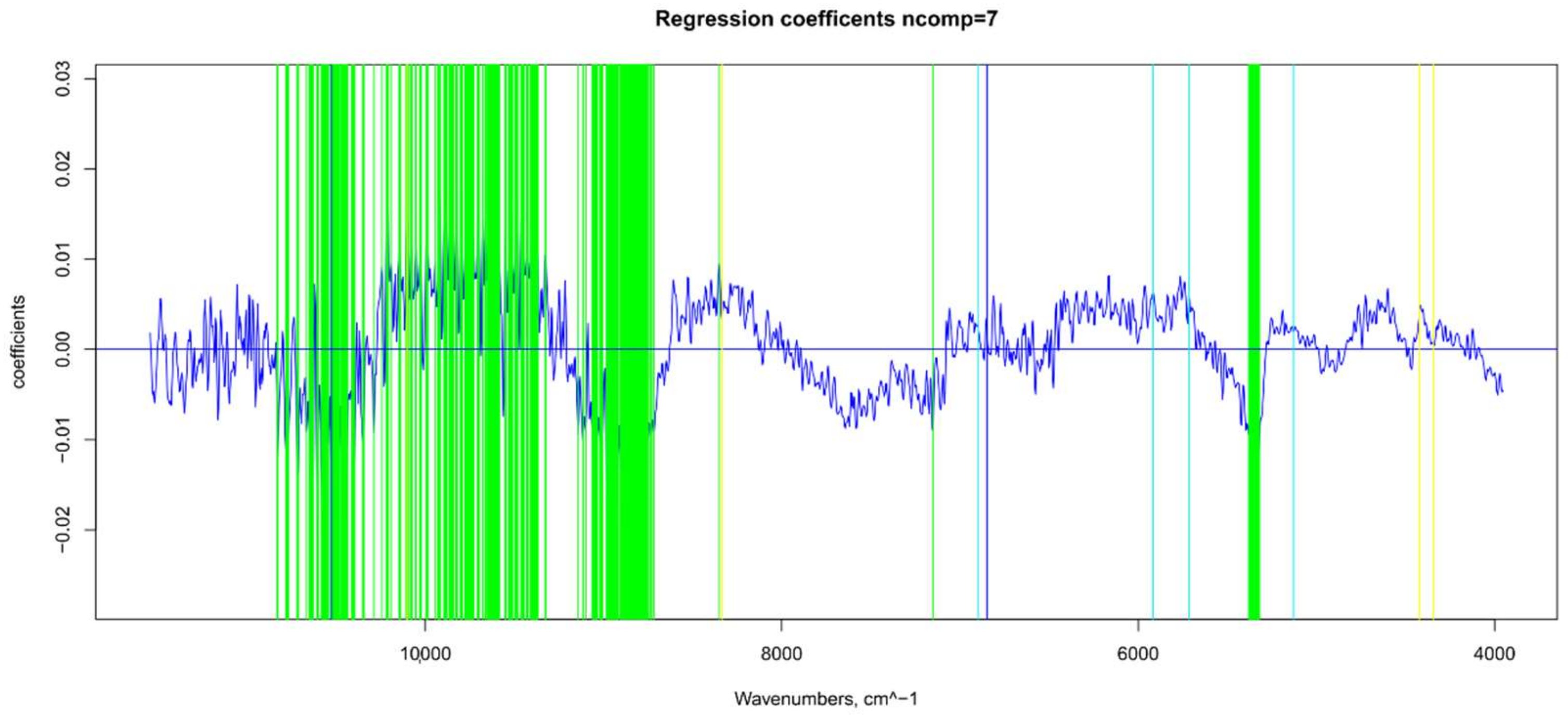
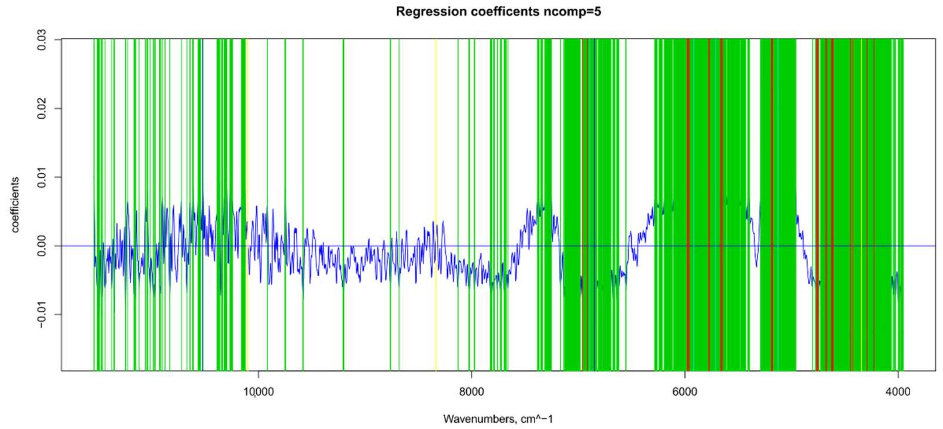
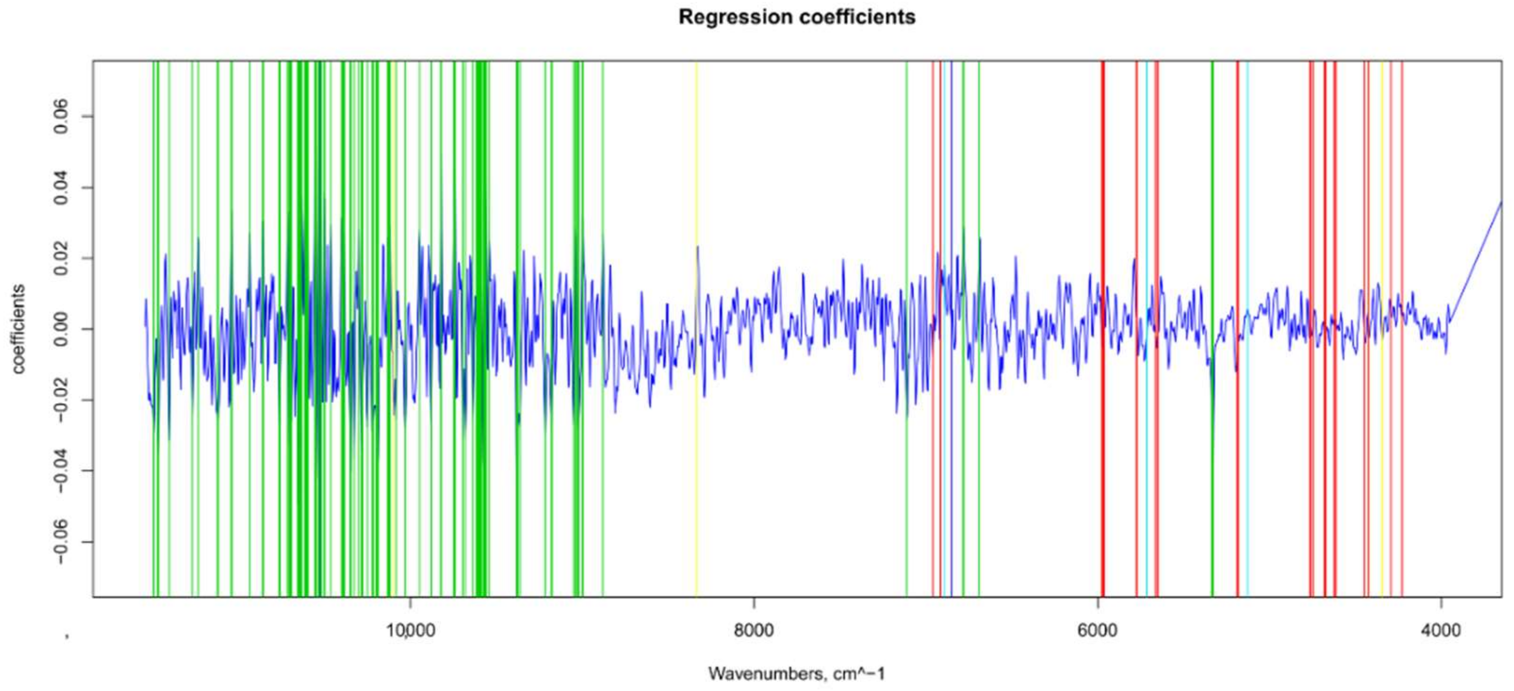
2.7.1. Βeta-Coefficients and MC-UVE
2.7.2. Data Normalization and Split into Training and Test Sets
2.7.3. PLS Models
2.7.4. ANN Structure
3. Results and Discussion
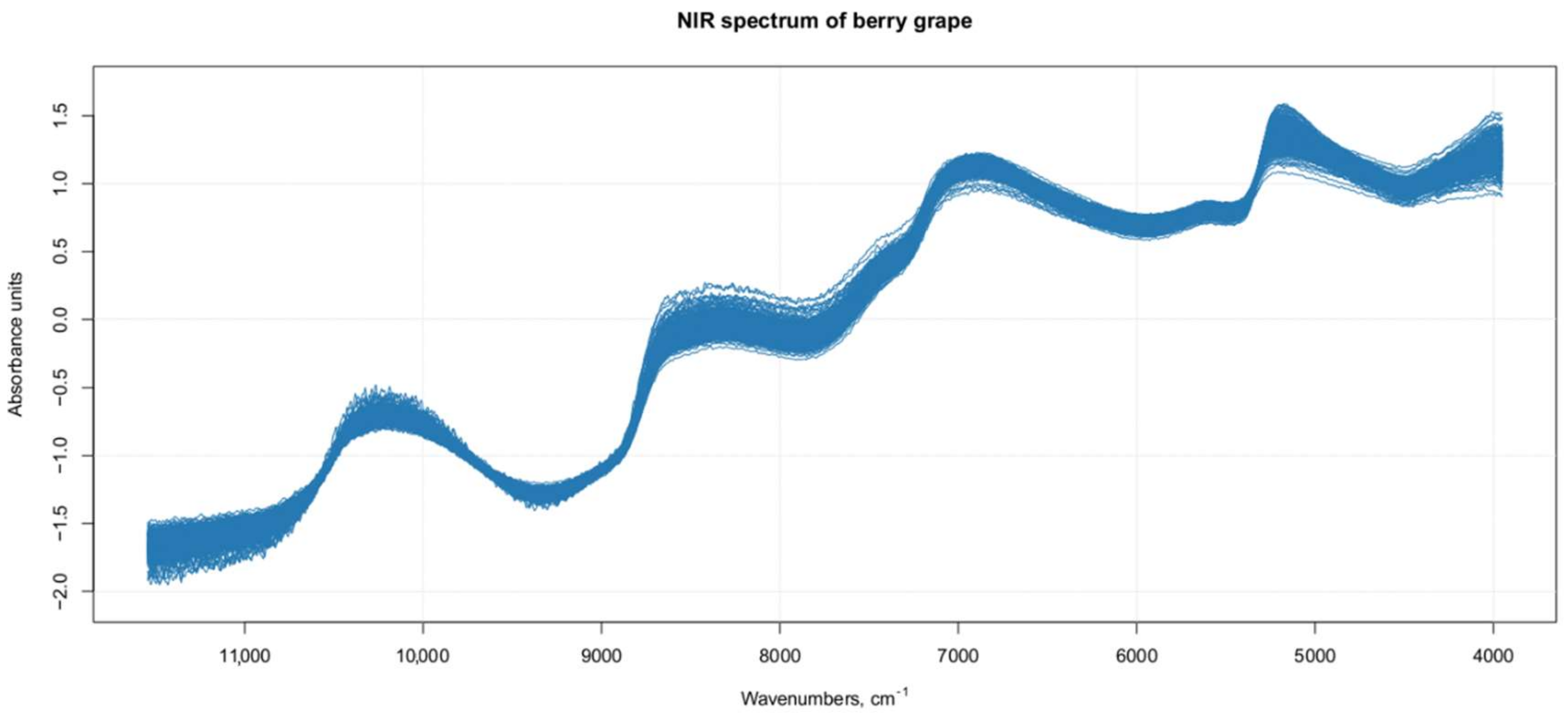
3.1. Raw NIR Spectral Analysis
3.2. Prediction of Unknown Samples
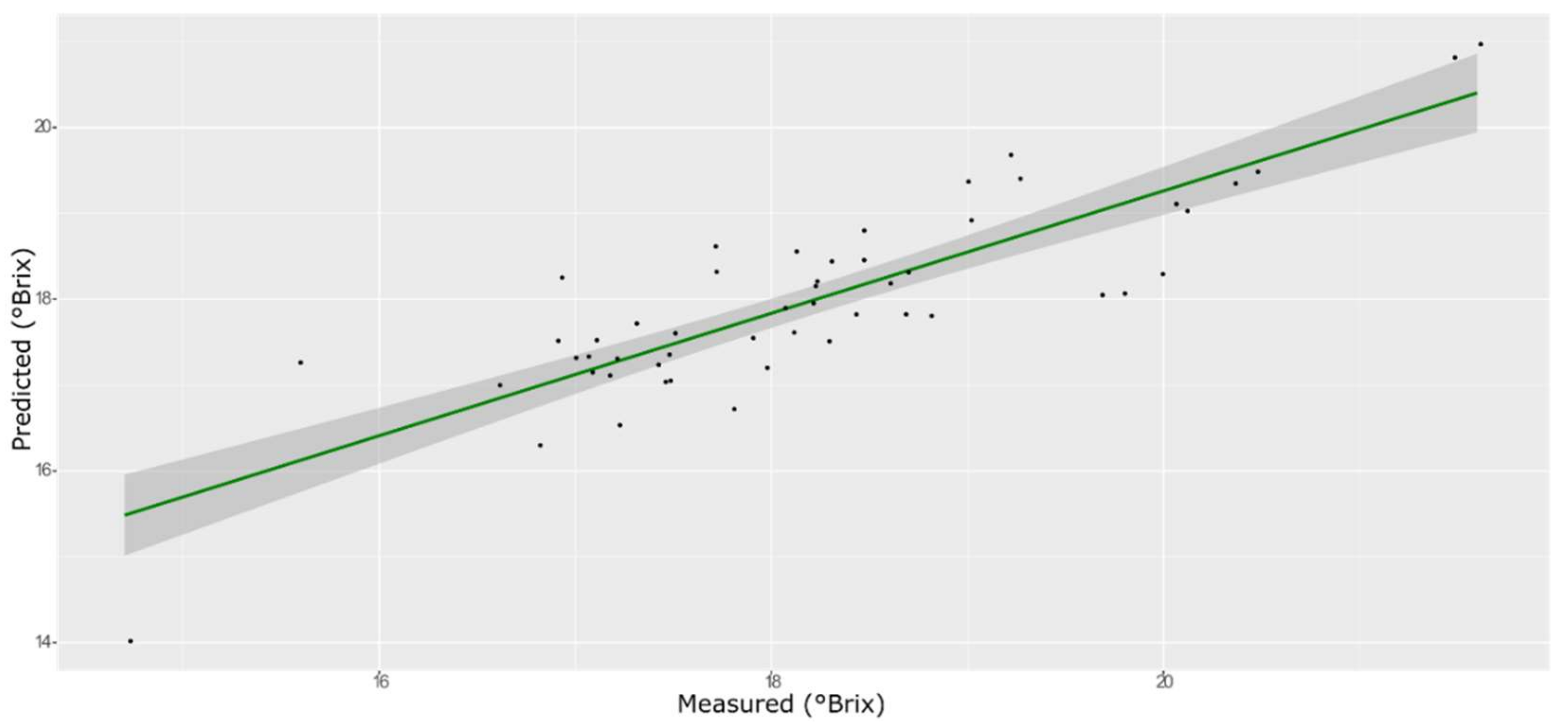
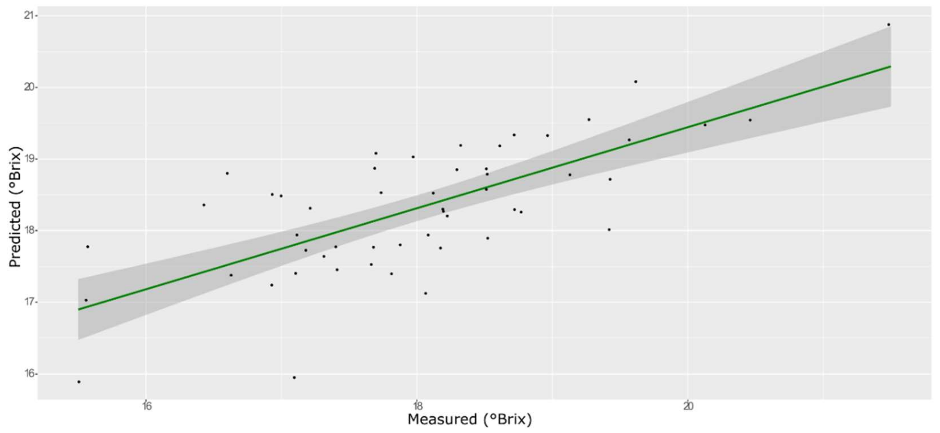
3.3. TSS Model
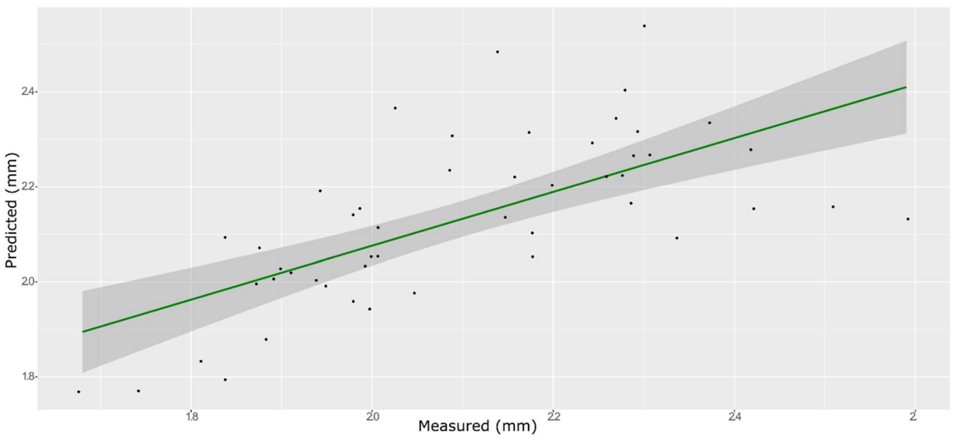
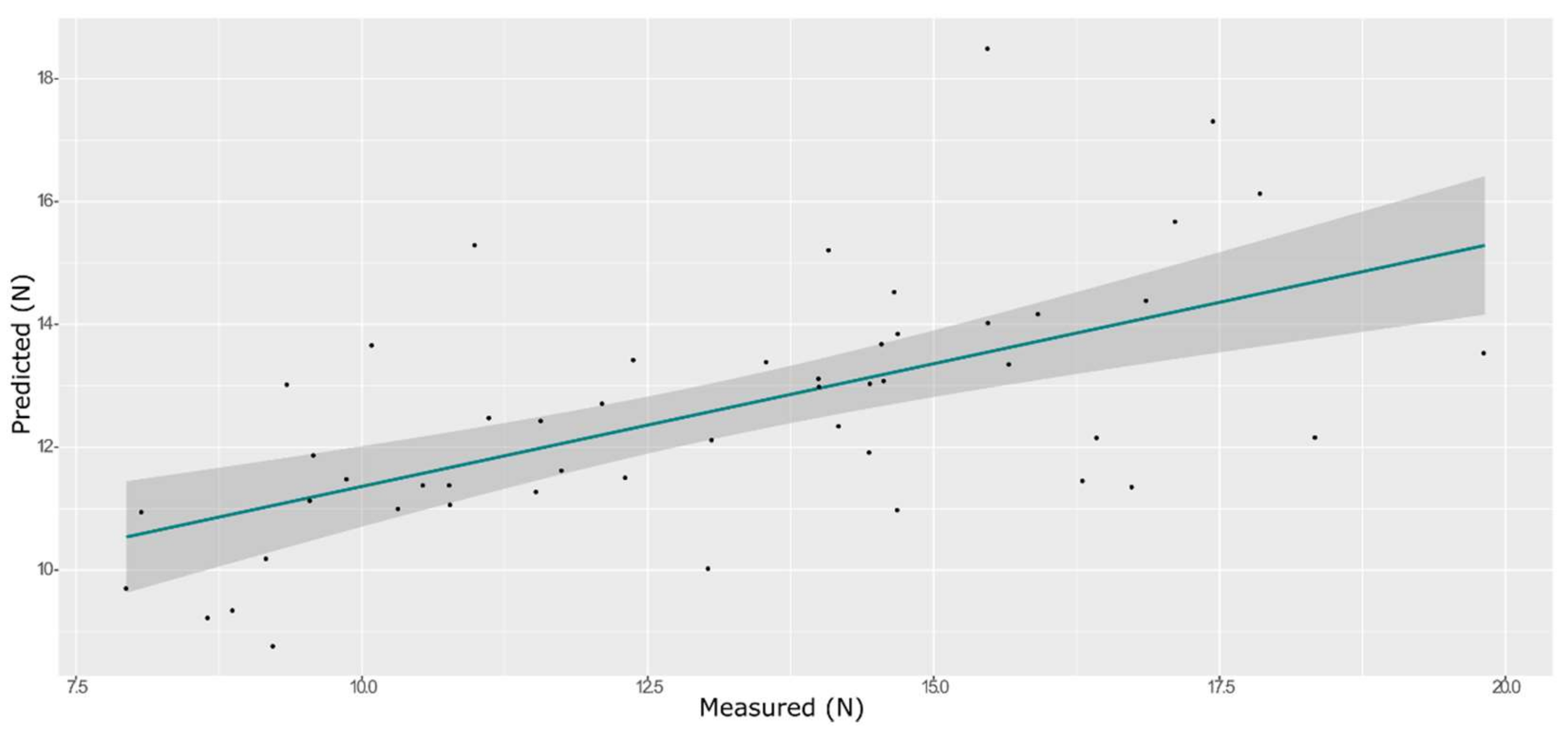
3.4. Springiness
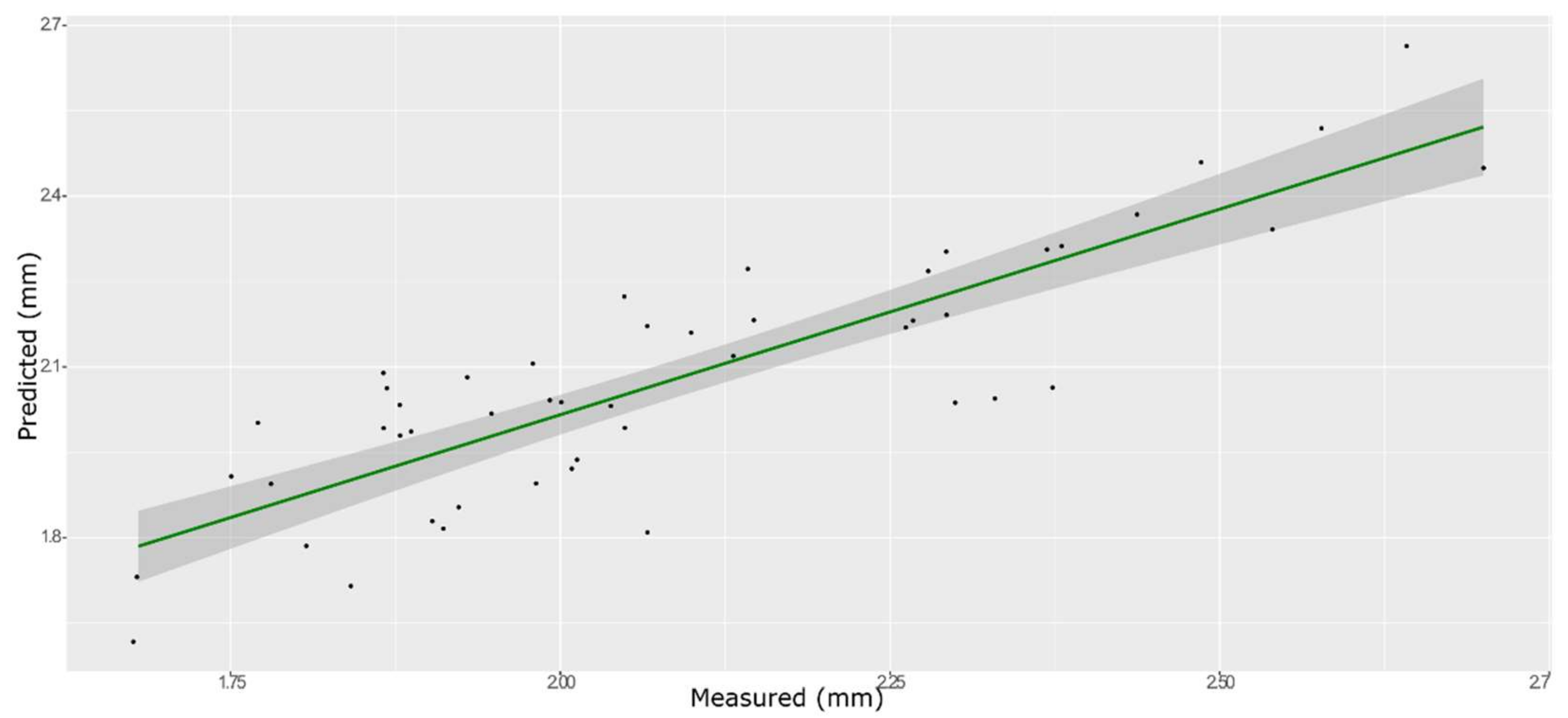
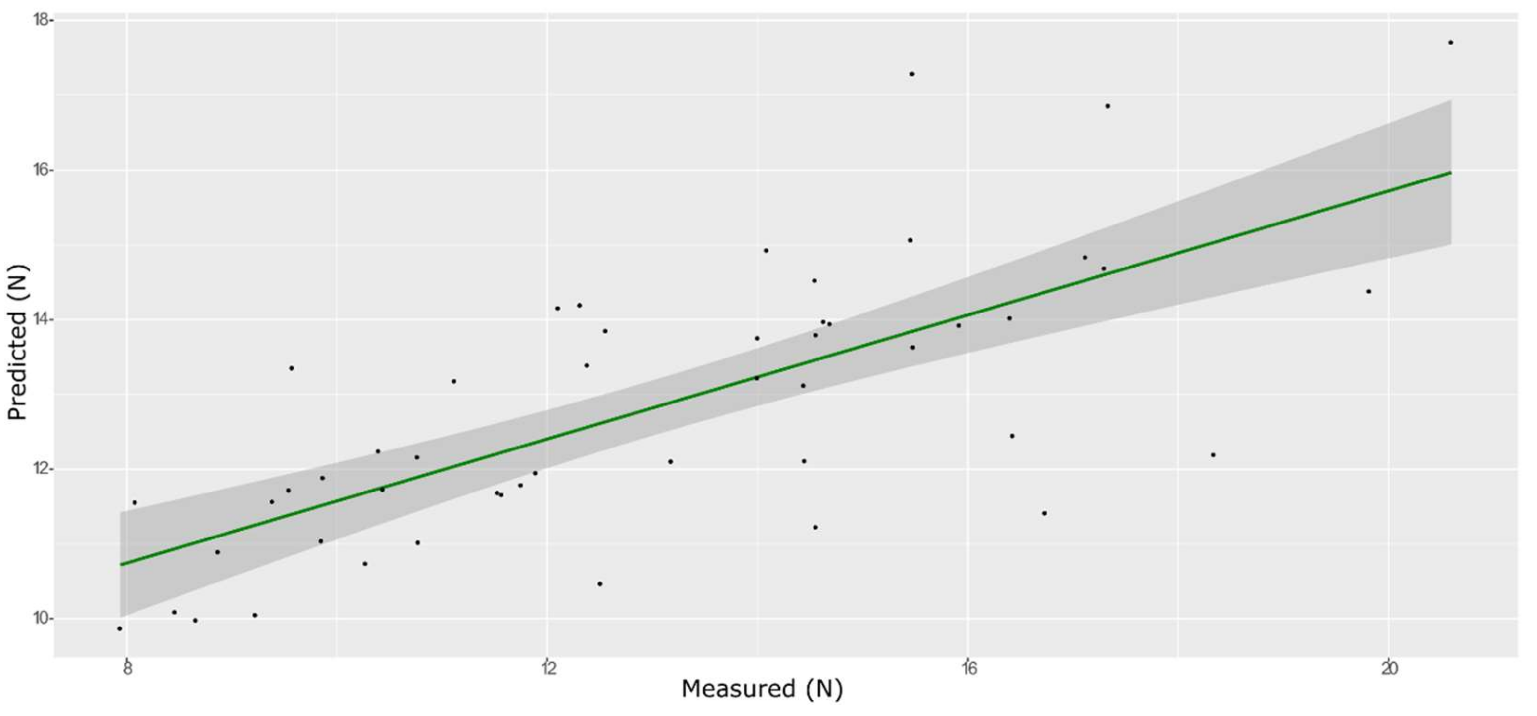
3.5. Hardness
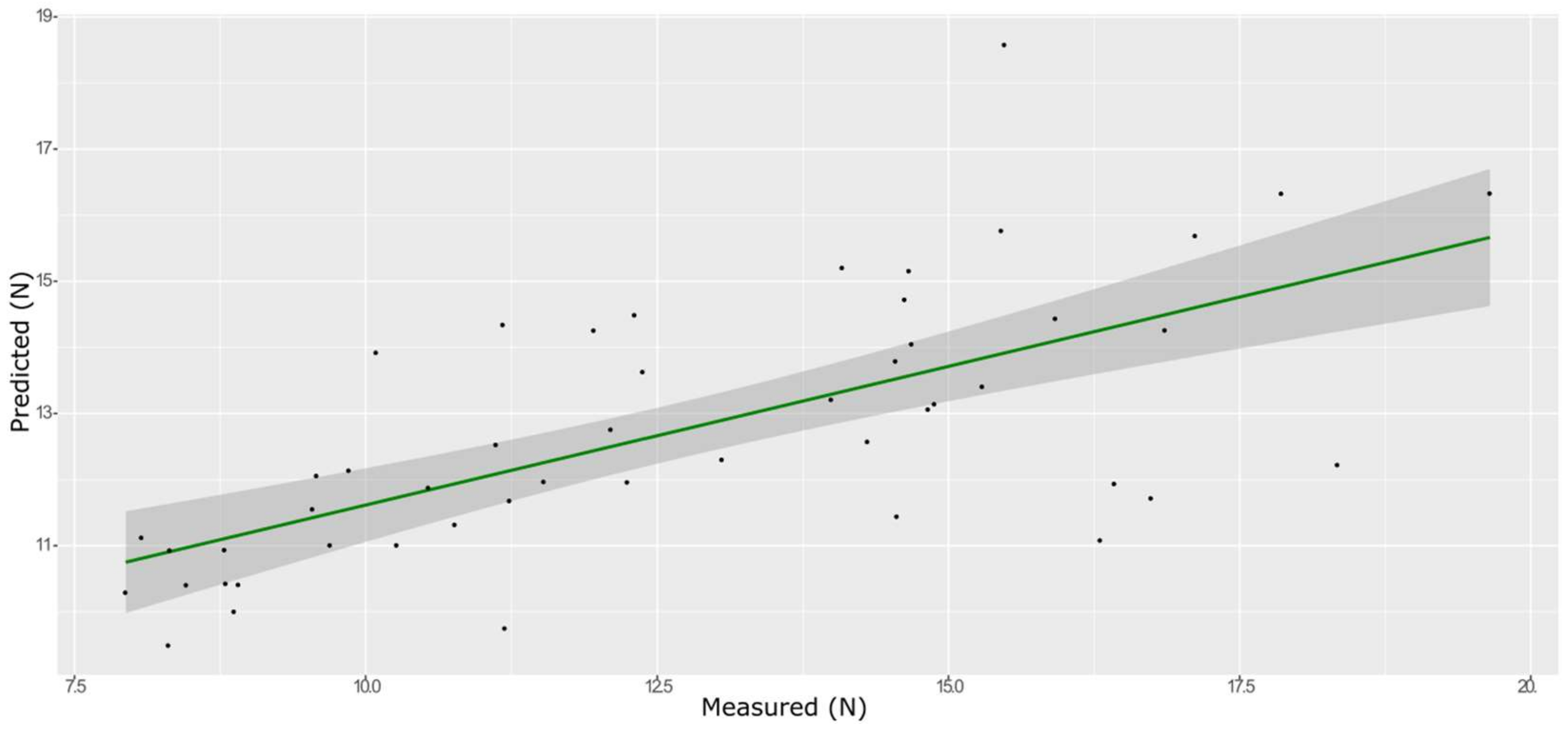
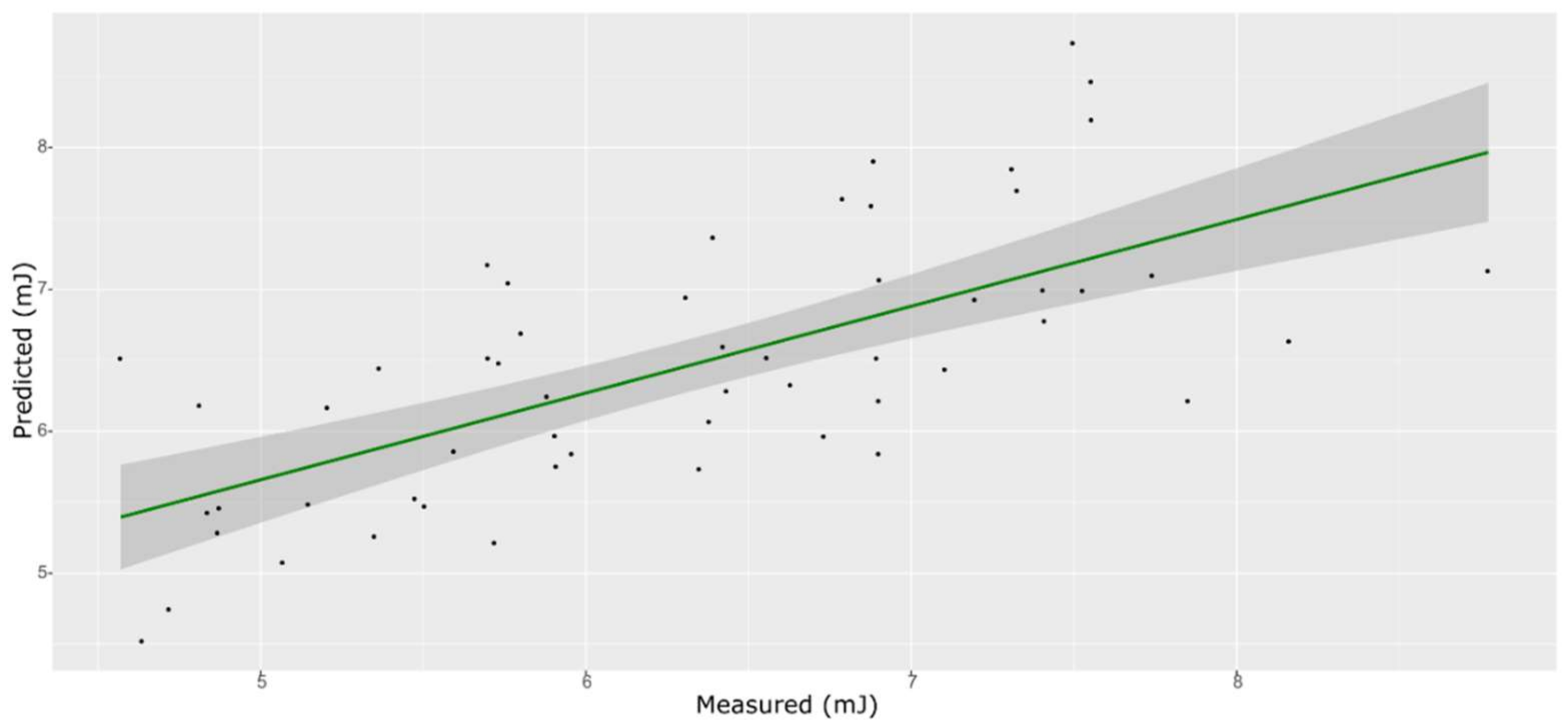
3.6. Chewiness
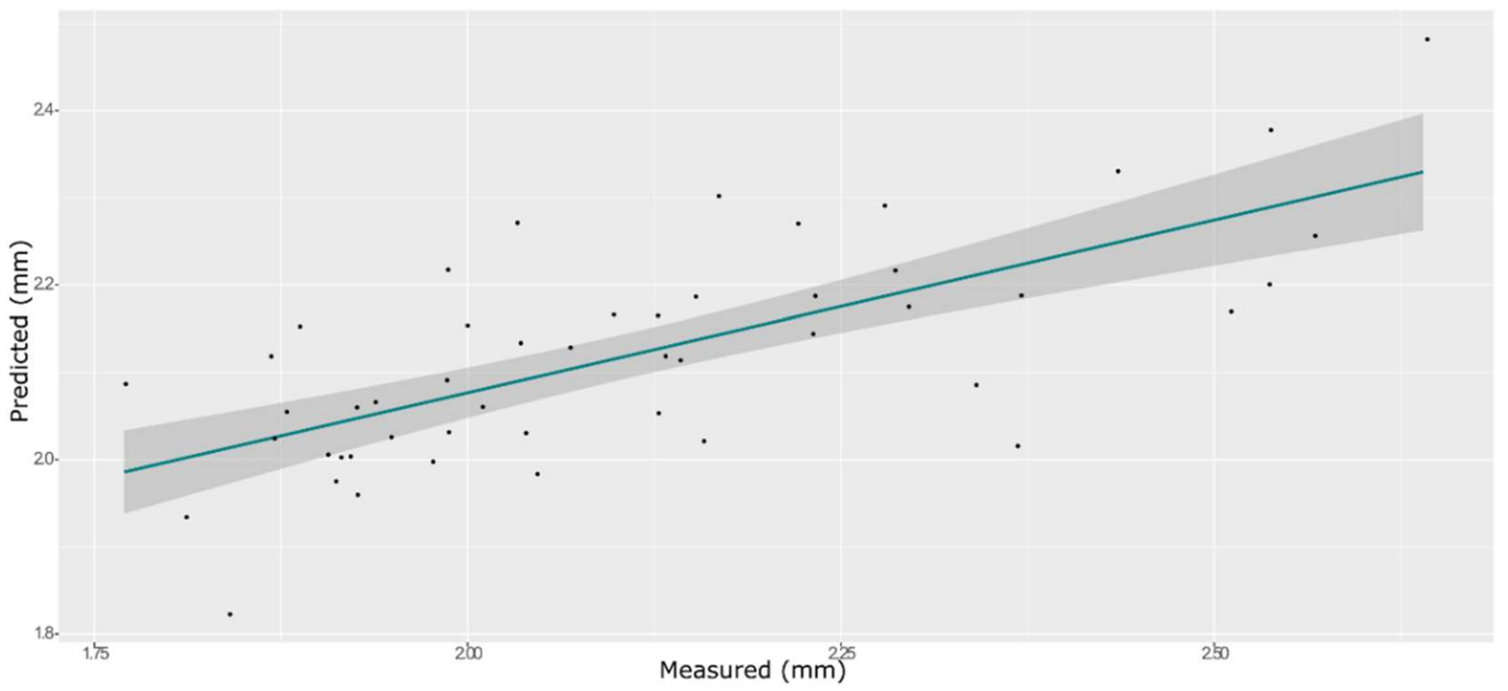
3.7. Cohesiveness
4. Conclusions
Supplementary Materials
Author Contributions
Funding
Institutional Review Board Statement
Informed Consent Statement
Data Availability Statement
Conflicts of Interest
References
- Fuentes, S.; Manso, A.; Fenoll, J.; Cava, J.; Garrido, I.; Molina, M.V.; Flores, P.; Hellín, P. Optimizing the methodology to measure firmness of grape berries (Vitis vinifera L.) during ripening. Acta Hortic. 2018, 1194, 1103–1110. [Google Scholar] [CrossRef]
- Basile, T.; Marsico, A.D.; Cardone, M.F.; Antonacci, D.; Perniola, R. FT-NIR analysis of intact table grape berries to understand consumer preference driving factors. Foods 2020, 9, 98. [Google Scholar] [CrossRef] [Green Version]
- Giacosa, S.; Zeppa, G.; Baiano, A.; Torchio, F.; Segade, S.R.; Gerbi, V.; Rolle, L. Assessment of sensory firmness and crunchiness of tablegrapes by acoustic and mechanical properties. Aust. J. Grape Wine Res. 2015, 21, 213–225. [Google Scholar] [CrossRef]
- Association de Coordination Technique pour l’Industrie Agro-Alimentaire (ACTIA). Sensory Evaluation Guide of Good Practice: Technical Report; Technical Coordination Association for the Food Industry: Paris, France, 2001; Available online: http://www.actia-asso.eu/cms/rubrique-2085-sensory_evaluation.html (accessed on 1 September 2021).
- Mancini, M.; Mazzoni, L.; Gagliardi, F.; Balducci, F.; Duca, D.; Toscano, G.; Mezzetti, B.; Capocasa, F. Application of the non-destructive NIR technique for the evaluation of strawberry fruits quality parameters. Foods 2020, 9, 441. [Google Scholar] [CrossRef] [PubMed] [Green Version]
- Bampi, M.; de Scheer, A.P.; Castilhos, F. Application of near infrared spectroscopy to predict the average droplet size and water content in biodiesel emulsions. Fuel 2013, 113, 546–552. [Google Scholar] [CrossRef] [Green Version]
- Conzen, J.P. Multivariate Calibration, 3rd ed.; Bruker Optik GmbH: Ettlingen, Germany, 2014; ISBN 9783929431131. [Google Scholar]
- Marsico, A.D.; Perniola, R.; Cardone, M.F.; Velenosi, M.; Antonacci, D.; Alba, V.; Basile, T. Study of the Influence of different yeast strains on red wine fermentation with NIR spectroscopy and principal component analysis. J 2018, 1, 13. [Google Scholar] [CrossRef] [Green Version]
- Wang, P.; Yu, Z. Species authentication and geographical origin discrimination of herbal medicines by near infrared spectroscopy: A review. J. Pharm. Anal. 2015, 5, 277–284. [Google Scholar] [CrossRef] [Green Version]
- Boeriu, C.G.; Stolle-Smits, T.; van Dijk, C. Characterisation of cell wall pectins by near infrared spectroscopy. J. Near Infrared Spectrosc. 1998, 6, A299–A301. [Google Scholar] [CrossRef]
- Basile, T.; Marsico, A.D.; Perniola, R. NIR analysis of intact grape berries: Chemical and physical properties prediction using multivariate analysis. Foods 2021, 10, 113. [Google Scholar] [CrossRef]
- Liu, W.; Yang, W.; Liu, L.; Yu, Q. Use of artificial neural networks in near-infrared spectroscopy calibrations for predicting glucose concentration in urine. In Proceedings of the 2008 International Conference on Intelligent Computing (ICIC 2008), Shanghai, China, 15–18 September 2008; Huang, D.S., Wunsch, D.C., Levine, D.S., Jo, K.H., Eds.; Springer: Berlin/Heidelberg, Germany; Volume 5226, pp. 1040–1046. [CrossRef]
- Büchmann, N.B.; Josefsson, H.; Cowe, I.A. Performance of European Artificial Neural Network (ANN) calibrations for moisture and protein in cereals using the danish Near-Infrared Transmission (NIT) network. Cereal Chem. J. 2001, 78, 572–577. [Google Scholar] [CrossRef]
- Zouid, I.; Siret, R.; Jourjon, F.; Mehinagic, E.; Rolle, L. Impact of grapes heterogeneity according to sugar level on both physical and mechanical berries properties and their anthocyanins extractability at harvest. J. Text. Stud. 2013, 44, 95–103. [Google Scholar] [CrossRef]
- Rolle, L.; Siret, R.; Segade, S.R.; Maury, C.; Gerbi, V.; Jourjon, F. Instrumental texture analysis parameters as markers of table-grape and winegrape quality: A review. Am. J. Enol. Vitic. 2012, 63, 11–28. [Google Scholar] [CrossRef] [Green Version]
- R Core Team. R: A Language and Environment for Statistical Computing, R Version 3.6.3; R Foundation for Statistical Computing: Vienna, Austria, 2020; Available online: https://www.R-project.org/ (accessed on 1 September 2021).
- Luedeling, E. Package “chillR”, Version 0.72.2, Title Statistical Methods for Phenology Analysis in Temperate Fruit Trees, 6 January 2021. Available online: https://cran.r-project.org/web/packages/chillR/chillR.pdf (accessed on 1 September 2021).
- Coombes, K.R.; Fritsche, H.A.; Clarke, C.; Chen, J.-N.; Baggerly, K.A.; Morris, J.S.; Xiao, L.-C.; Hung, M.-C.; Kuerer, H.M.; Arndt, T. Quality control and peak finding for proteomics data collected from nipple aspirate fluid by surface-enhanced laser desorption and ionization. Clin. Chem. 2003, 49, 1615–1623. [Google Scholar] [CrossRef]
- Xiao, N.; Cao, D.-S.; Li, M.-Z.; Xu, Q.-S. Package “enpls”, Version 6.1, Title Ensemble Partial Least Squares Regression, 18 May 2019. Available online: https://cran.r-project.org/web/packages/enpls/enpls.pdf (accessed on 1 September 2021).
- Vu, V.Q.; ggbiplot. A ggplot2 Based Biplot R Package: Version 0.55. 2011. Available online: http://github.com/vqv/ggbiplot552 (accessed on 1 September 2021).
- Wickham, H.; Chang, W.; Henry, L.; Pedersen, T.L.; Takahashi, K.; Wilke, C.; Woo, K.; Yutani, H.; Dunnington, D. Package “ggplot2”, Version 3.3.3, Title Create Elegant Data Visualisations Using the Grammar of Graphics, 30 December 2020. Available online: https://cran.r-project.org/web/packages/ggplot2/ggplot2.pdf (accessed on 1 September 2021).
- Falbel, D.; Allaire, J.J.; Chollet, F.; Tang, Y.; Van Der Bijl, W.; Studer, M.; Keydana, S. Package “keras”, Version 2.4.0, Title R Interface to “Keras”, 29 March 2021. Available online: https://cran.r-project.org/web/packages/keras/keras.pdf (accessed on 1 September 2021).
- Kucheryavskiy, S. mdatools—R package for chemometrics. Chemom. Intell. Lab. Syst. 2020, 198, 103937. [Google Scholar] [CrossRef]
- Hamner, B.; Frasco, M.; Le Dell, E. Package “Metrics’, Version 0.1.4, Title Evaluation Metrics for Machine Learning, 9 July 2018. Available online: https://cran.r-project.org/web/packages/Metrics/Metrics.pdf (accessed on 1 September 2021).
- Stevens, A.; Ramirez-Lopez, L. An Introduction to the Prospectr Package: R Package Vignette R Package Version 0.2.1. 2020. Available online: https://cran.r-project.org/web/packages/prospectr/vignettes/prospectr.html (accessed on 1 September 2021).
- Signal Developers. Signal: Signal Processing. 2013. Available online: http://r-forge.r-project.org/projects/signal/ (accessed on 1 September 2021).
- Chalmers, P.; Sigal, M.; Oguzhan, O. Package “SimDesign”, Version 2.3, Title Structure for Organizing Monte Carlo Simulation Designs, 7 April 2021. Available online: https://cran.csiro.au/web/packages/SimDesign/SimDesign.pdf (accessed on 1 September 2021).
- Engel, J.; Gerretzen, J.; Szymańska, E.; Jansen, J.J.; Downey, G.; Blanchet, L.; Buydens, L.M.C. Breaking with trends in pre-processing? TrAC Trends Anal. Chem. 2013, 50, 96–106. [Google Scholar] [CrossRef]
- Pomerantsev, A.L.; Rodionova, O.Y. Concept and role of extreme objects in PCA/SIMCA. J. Chemom. 2014, 28, 429–438. [Google Scholar] [CrossRef]
- Gestal, M.; Gómez-Carracedo, M.P.; Andrade, J.M.; Dorado, J.; Fernández, E.; Prada, D.; Pazos, A. Classification of apple beverages using artificial neural networks with previous variable selection. Anal. Chim. Acta 2004, 524, 225–234. [Google Scholar] [CrossRef]
- Cai, W.; Li, Y.; Shao, X. A variable selection method based on uninformative variable elimination for multivariate calibration of near-infrared spectra. Chemom. Intell. Lab. Syst. 2008, 90, 188–194. [Google Scholar] [CrossRef]
- Fan, W.; Shan, Y.; Li, G.; Lv, H.; Li, H.; Liang, Y. Application of competitive adaptive reweighted sampling method to determine effective wavelengths for prediction of total acid of vinegar. Food Anal. Methods 2012, 5, 585–590. [Google Scholar] [CrossRef]
- Martelo-Vidal, M.J.; Vazquez, M. Application of artificial neural networks coupled to UV–VIS–NIR spectroscopy for the rapid quantification of wine compounds in aqueous mixtures. CyTA J. Food 2015, 13, 32–39. [Google Scholar] [CrossRef] [Green Version]
- Rodionova, O.Y.; Pomerantsev, A.L. Detection of outliers in projection-based modeling. Anal. Chem. 2020, 92, 2656–2664. [Google Scholar] [CrossRef]
- Pomerantsev, A.L. Acceptance areas for multivariate classification derived by projection methods. J. Chemom. 2008, 22, 601–609. [Google Scholar] [CrossRef]
- Zaukuu, J.-L.Z.; Soós, J.; Bodor, Z.; Felföldi, J.; Magyar, I.; Kovacs, Z. Authentication of Tokaj wine (Hungaricum) with the electronic tongue and near infrared spectroscopy. J. Food Sci. 2019, 84, 3437–3444. [Google Scholar] [CrossRef] [PubMed]
- Cozzolino, D.; Cynkar, W.; Shah, N.; Smith, P. Quantitative analysis of minerals and electric conductivity of red grape homogenates by near infrared reflectance spectroscopy. Comput. Electron. Agric. 2011, 77, 81–85. [Google Scholar] [CrossRef]
- Martelo-Vidal, M.J.; Vázquez, M. Evaluation of ultraviolet, visible and near infrared spectroscopy for the analysis of wine compounds. Czech J. Food Sci. 2014, 32, 37–47. [Google Scholar] [CrossRef] [Green Version]
- Shen, F.; Yang, D.T.; Ying, Y.B.; Li, B.B.; Zheng, Y.F.; Jiang, T. Discrimination between Shaoxing wines and other Chinese rice wines by near-infrared spectroscopy and chemometrics. Food Bioprocess Technol. 2012, 5, 786–795. [Google Scholar] [CrossRef]
- Liu, F.; He, Y.; Wang, L.; Sun, G. Detection of organic acids and pH of fruit vinegars using near-infrared spectroscopy and multivariate calibration. Food Bioprocess Technol. 2011, 4, 1331–1340. [Google Scholar] [CrossRef]
- Beghi, R.; Giovenzana, V.; Marai, S.; Guidetti, R. Rapid monitoring of grape withering using visible near-infrared spectroscopy. J. Sci. Food Agric. 2015, 95, 3144–3149. [Google Scholar] [CrossRef]
- Giovenzana, V.; Civelli, R.; Beghi, R.; Oberti, R.; Guidetti, R. Testing of a simplified LED based vis/NIR system for rapid ripeness evaluation of white grape (Vitis vinifera L.) for Franciacorta wine. Talanta 2015, 144, 584–591. [Google Scholar] [CrossRef] [PubMed]
- Crespan, M.; Migliaro, D.; Vezzulli, S.; Zenoni, S.; Tornielli, G.B.; Giacosa, S.; Paissoni, M.A.; Segade, S.R.; Rolle, L. A major QTL is associated with berry grape texture characteristics. OENO One 2021, 55, 183–206. [Google Scholar] [CrossRef]
- Higdon, R. Experimental design, variability. In Encyclopedia of Systems Biology; Dubitzky, W., Wolkenhauer, O., Cho, K.-H., Yokota, H., Eds.; Springer: New York, NY, USA, 2013; pp. 704–705. [Google Scholar] [CrossRef]
- Chung, H. Applications of near-infrared spectroscopy in refineries and important issues to address. Appl. Spectrosc. Rev. 2007, 42, 251–285. [Google Scholar] [CrossRef]
- Rahman, M.S.; Al-Farsi, S.A. Instrumental texture profile analysis (TPA) of date flesh as a function of moisture content. J. Food Eng. 2005, 66, 505–511. [Google Scholar] [CrossRef]
- Moore, J.P.; Fangel, J.U.; Willats, W.G.T.; Vivier, M.A. Pectic-β(1,4)-galactan, extensin and arabinogalactan–protein epitopes differentiate ripening stages in wine and table grape cell walls. Ann. Bot. 2014, 114, 1279–1294. [Google Scholar] [CrossRef] [PubMed] [Green Version]
- Overview of Texture Profile Analysis. Available online: https://texturetechnologies.com/resources/texture-profile-analysis#settings-and-standards (accessed on 1 September 2021).
- Martynenko, A.; Janaszek-Mańkowska, M.A. Texture changes during drying of apple slices. Dry. Technol. 2014, 32, 567–577. [Google Scholar] [CrossRef]
- Cauvain, S.P. Bread and other bakery products. In The Stability and Shelf Life of Food, 2nd ed.; Subramaniam, P., Ed.; Woodhead Publishing: Sawston, UK, 2016; pp. 431–459. ISBN 9780081004357. [Google Scholar]
- Di Monaco, R.; Cavella, S.; Masi, P. Predicting sensory cohesiveness, hardness and springiness of solid foods from instrumental measurements. J. Text. Stud. 2008, 39, 129–149. [Google Scholar] [CrossRef]


| Model | Spectra | R2 | RMSE | Bias | RPD |
|---|---|---|---|---|---|
| PLS Entire spectrum (nComp 7) | Training with CV | 0.69 | 1.02 | 0.004 | 2.33 |
| External validation | 0.69 | 0.74 | 0.225 | 1.91 | |
| PLS Selected wavenumbers (nComp 4) | Training with CV | 0.74 | 0.95 | 0.007 | 1.95 |
| External validation | 0.46 | 0.87 | −0.303 | 1.46 | |
| ANN | Training with CV | 0.93 | 0.50 | −0.132 | 3.66 |
| External validation | 0.82 | 0.52 | −0.048 | 2.35 |
| Model | Spectra | R2 | RMSE | Bias | RPD |
|---|---|---|---|---|---|
| PLS Entire spectrum (nComp8) | Training with CV | 0.430 | 0.191 | 0.0010 | 1.33 |
| External validation | 0.394 | 0.160 | −0.0324 | 1.33 | |
| PLS Selected wavenumbers (nComp 2) | Training with CV | 0.591 | 0.161 | 0.0005 | 1.57 |
| External validation | 0.473 | 0.159 | −0.0087 | 1.39 | |
| ANN | Training with CV | 0.899 | 0.191 | −0.1079 | 2.56 |
| External validation | 0.724 | 0.133 | −0.0094 | 1.94 |
| Model | Spectra | R2 | RMSE | Bias | RPD |
|---|---|---|---|---|---|
| PLS Entire spectrum (nComp 6) | Training with CV | 0.44 | 2.49 | −0.007 | 1.34 |
| External validation | 0.44 | 2.32 | −0.061 | 1.35 | |
| PLS Selected wavenumbers (nComp 8) | Training with CV | 0.54 | 2.27 | −0.002 | 1.49 |
| External validation | 0.42 | 2.28 | 0.618 | 1.37 | |
| ANN | Training with CV | 0.49 | 2.38 | −0.022 | 1.40 |
| External validation | 0.50 | 2.24 | −0.198 | 1.41 |
| Model | Spectra | R2 | RMSE | Bias | RPD |
|---|---|---|---|---|---|
| PLS Entire spectrum (nComp7) | Training with CV | 0.545 | 1.096 | 0.0027 | 1.49 |
| External validation | 0.383 | 0.790 | −0.1506 | 1.31 | |
| PLS Selected wavenumbers (nComp 5) | Training with CV | 0.604 | 1.002 | −0.0053 | 1.59 |
| External validation | 0.436 | 0.910 | −0.0926 | 1.35 | |
| ANN | Training with CV | 0.900 | 0.505 | −0.2082 | 2.90 |
| External validation | 0.530 | 1.176 | 0.0017 | 1.48 |
Publisher’s Note: MDPI stays neutral with regard to jurisdictional claims in published maps and institutional affiliations. |
© 2022 by the authors. Licensee MDPI, Basel, Switzerland. This article is an open access article distributed under the terms and conditions of the Creative Commons Attribution (CC BY) license (https://creativecommons.org/licenses/by/4.0/).
Share and Cite
Basile, T.; Marsico, A.D.; Perniola, R. Use of Artificial Neural Networks and NIR Spectroscopy for Non-Destructive Grape Texture Prediction. Foods 2022, 11, 281. https://doi.org/10.3390/foods11030281
Basile T, Marsico AD, Perniola R. Use of Artificial Neural Networks and NIR Spectroscopy for Non-Destructive Grape Texture Prediction. Foods. 2022; 11(3):281. https://doi.org/10.3390/foods11030281
Chicago/Turabian StyleBasile, Teodora, Antonio Domenico Marsico, and Rocco Perniola. 2022. "Use of Artificial Neural Networks and NIR Spectroscopy for Non-Destructive Grape Texture Prediction" Foods 11, no. 3: 281. https://doi.org/10.3390/foods11030281
APA StyleBasile, T., Marsico, A. D., & Perniola, R. (2022). Use of Artificial Neural Networks and NIR Spectroscopy for Non-Destructive Grape Texture Prediction. Foods, 11(3), 281. https://doi.org/10.3390/foods11030281