Abstract
The intervertebral discs (IVD) are among the essential organs of the human body, ensuring the mobility of the spine. These organs possess a high proportion of water. However, as the discs age, this content decreases, which can potentially lead to various diseases called degenerative disc diseases. This water content is therefore an important indicator of the well-being of the disc. In this paper, we propose photoacoustic imaging as a means of probing a disc and quantitatively recovering its molecular composition, which should allow concluding on its state. An adjoint-assisted gradient descent scheme is implemented to recover the optical absorption coefficient in the disc, from which, if spectroscopic measurements are performed, the molecular composition can be deduced. The algorithm was tested on synthetic measurements. A realistic numerical phantom was built from magnetic resonance imaging of an actual IVD of a pig. A simplified experiment, with a single laser source, was performed. Results show the feasibility of using photoacoustics imaging to probe IVDs. The influences of exact and approximate formulations of the gradient are studied. The impact of noise on the reconstructions is also evaluated.
1. Introduction
The intervertebral discs (IVD) are fibrocartilaginous organs present between the vertebrae of the spine. Together, they ensure the mobility of the back and act as shock absorbers. These organs contain a high percentage of water [1]. However, as time goes by, they progressively lose their water content. This perfectly natural process can lead to degenerative disc diseases [2] and pain. Low back pain is one of the most common consequences of the degeneration of the discs, and has important social and economical consequences in today’s society [3].
The current prevalent treatment options are disc excision and spinal fusion. These options are not without consequences, as they lower the mobility of the spinal column, but most importantly, they accelerate the degeneration process in the neighbouring discs due to the altered mechanics of the spine [4]. Consequently, new promising treatment options are currently being investigated, such as the development of hydrogels for the replacement of degenerated discs [5].
In terms of diagnosis of discs, magnetic resonance imaging (MRI) is most commonly used for pathology assessment [6]. It allows for good quantitative estimation of the main components of a disc. Computerised tomography (CT) is another commonly used technique that provides complementary information. However, both techniques are time-consuming, expensive and not transportable to the operating room. Hence the need for more flexible techniques able to provide quick and accurate diagnosis on IVD viability.
Optical imaging techniques such as photoacoustic (PA) imaging could offer alternatives with which to probe the discs. PA measurements of a pig’s IVD performed in a previous study [7] hinted at this possibility: the PA signals obtained showed significant variations with the water content of the disc, meaning that its content could be recovered with this technique. PA imaging makes use of a pulsed laser to create an acoustic pressure rise in tissues that propagates and can then be detected with acoustic sensors. From PA measurements of the disc, it is possible to recover the optical properties and related parameters, such as the chromophore distribution, which allows us to assess the state of an IVD: this is the aim of quantitative photoacoustic imaging (QPAI).
To this end, two inverse problems need to be solved in QPAI: the acoustic inverse problem, which is the recovery of the initial pressure rise in the tissue from the detected acoustic signal, and the optical inverse problem, which corresponds to the recovery of the optical properties of the tissue from the initial pressure distribution. In this paper, we restrict ourselves to the resolution of the optical inverse problem for IVDs.
To solve the QPAI inverse optical problem, the method chosen in the present study is the gradient descent scheme method. This approach allows for the reconstruction of parameters of interest through the minimisation of an error function and can be employed for large scale problems with many variables, which is the case in the realistic scenario of three-dimensional (3D) QPAI. Gradient descent schemes have already been used to reconstruct optical parameters from photoacoustic measurements: Cox et al. [8] used a gradient descent scheme to recover the absorption or scattering coefficient when the other coefficient is known in a two-dimensional (2D) numerical phantom where two chromophore distributions are defined. They worked with the diffusion approximation model of light transport to reconstruct the chromophores concentration using the finite difference method. Hochuli et al. [9] presented a different 2D numerical study of QPAI in a simple phantom consisting of a background area in which squared areas with different optical properties were set up. The radiative light transport model was chosen and solved with Monte Carlo simulations. The absorption and scattering coefficients were recovered with prior knowledge of the other coefficient. More recently, Buchmann et al. [10] proposed a 3D numerical study where they recovered the concentration of the chromophores in a simulated tissue containing blood vessels using a multispectral radiance model. The radiative transfer model was also solved with Monte Carlo simulations. In their study, the scattering coefficient was supposed to be homogeneous and known a priori.
The purpose of the present article is to evaluate the feasibility of using PA imaging to probe a disc and assessing its state. To the best of our knowledge, this method has never been applied to the diagnosis of this organ before. To that end, a similar approach as [10] was adopted. A numerical study has been conducted to show the possibility of using PA to quantitatively reconstruct the optical properties of the IVD, and therefore conclude on its integrity. An adjoint-assisted gradient scheme algorithm was implemented for the resolution of the optical inverse problem. A radiance model, solved with Monte Carlo simulations, was chosen for its generality. We implemented the gradient descent scheme method in the very specific environment of the IVD. A realistic numerical phantom was built from MRI measurements of the IVD of a pig [11,12]. This organ possesses spatially-varying absorption and scattering coefficients, which add some complexities to the reconstruction of these optical properties, as the number of unknowns is much higher than in homogeneous media. In the 3D numerical model developed in the paper, the number of unknowns is equal to the number of voxels defining the disc, which is approximately 62,000 voxels. The present study is limited to the reconstruction of the absorption coefficient.
In this paper, we present first the necessary morphological and physiological information on IVDs in Section 2. PA theory and the definition of the forward model is presented in Section 3. The numerical phantom and the gradient descend approach implemented are described in Section 4. The results and associated discussion are in Section 5 and Section 6 respectively.
2. Morphology and Composition of the Intervertebral Disc
The IVD is composed of three main components: water, which is the most prevalent component; collagen (mainly type I and II); and proteoglycans. The IVD can be separated into two distinct zones. The central part of the disc is called the nucleus pulposus (NP) and is the most hydrated part of the disc. An healthy disc possesses a water proportion between 80% and 90% in this zone [13]. This central part is surrounded by the annulus fibrosus (AF), which is composed of about 15 to 25 concentric lamellae containing a highly structured pattern of collagen fibres [14]. In a healthy disc, the water content of the AF is between 65% and 70% [1]. In this particular zone, the water content decreases radially as one moves away from the NP [13,15].
In the scope of this paper, the IVD is considered a biphasic medium, composed of collagen and water only. The absorption and scattering coefficients are calculated using the proportion of chromophores at position r inside the disc. In the case of the simulated biphasic IVD, these coefficients depend on the wavelength and can be written using a mixing law as:
where is the scattering coefficient of collagen; and are the proportions at position r of collagen and water, respectively; and and are the specific absorption coefficients of collagen and water, respectively. The absorption and scattering coefficients of these two chromophores are presented in Figure 1 and were taken from [16]. In this reference, the optical properties of collagen were determined by diffuse optical spectroscopy.
Figure 1.
Absorption coefficients of collagen and water (left) and the scattering coefficient of collagen (right). Adapted from Ref. [16].
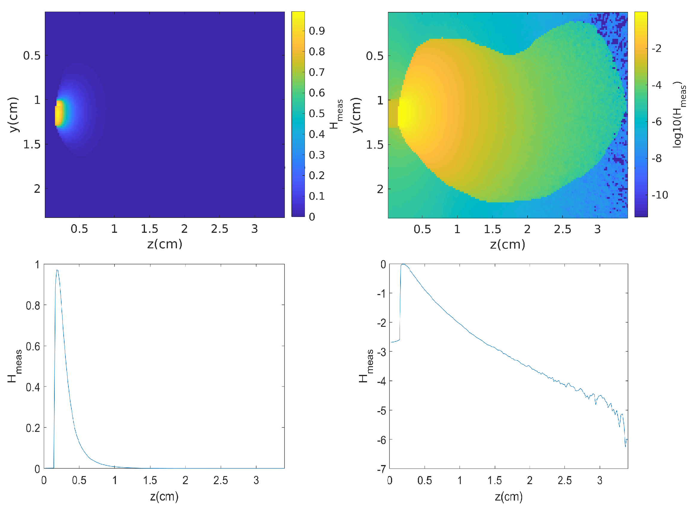
3. Photoacoustic Synthetic Measurements
In PA, a short-pulsed laser (a few nanoseconds for stress and thermal confinement approximations) is used to create a heat-induced acoustic pressure in the illuminated medium. This acoustic pressure then propagates and can be detected using acoustic sensors placed around the medium that measure a time-resolved photoacoustic response . The inverse problem in QPAI consists of recovering the optical properties of the medium from the set of photoacoustic responses . In this paper, we decompose this photoacoustic problem into two problems: the acoustic inverse problem, which is the recovery of the pressure rise instantaneously (short-pulsed laser) created by the laser at initial time from the time-resolved photoacoustic response (e.g., with time-reversal approaches); and the optical inverse problem, which is the recovery of the optical properties from the pressure rise . We focused on the resolution of the optical inverse problem; therefore, we simulated synthetic PA measurements of an IVD and supposed the acoustic inverse problem to be perfectly solved. In reality, the resolution of the acoustic inverse problem would give rise to errors in the recovered PA initial pressure rise due to, e.g., the limited bandwidth, the angular resolution of the acoustic sensors and artefacts linked to the reconstruction methods. The present study does not take these problems into account. Within the thermal and stress confinements (which are generally satisfied for nanosecond-pulsed lasers), the deposited laser energy density (W·cm) can be considered instantaneous and be written as:
with being the Dirac function. The problem can then be reformulated as an initial value problem with the PA pressure rise (Pa) at initial time described as:
is the Grüneisen parameter (); and are, respectively, the absorption and scattering coefficients (cm); g is the anisotropy factor (); is the fluence (W·cm). For simplicity, is supposed to be known and equal to 1 in this study. If needed, it has been shown that spectroscopic measurements allow one to account for it [17,18]. With this simplification, the measurement is referred to as from this point. The anisotropy coefficient g is supposed to be equal to 0.9 in the IVD and to 1 in water. Monte Carlo simulations are accurate at solving the radiative transfer equation, provided sufficient statistics are considered, and this method was chosen here to compute the fluence , with the versatile MCmatlab software [19].
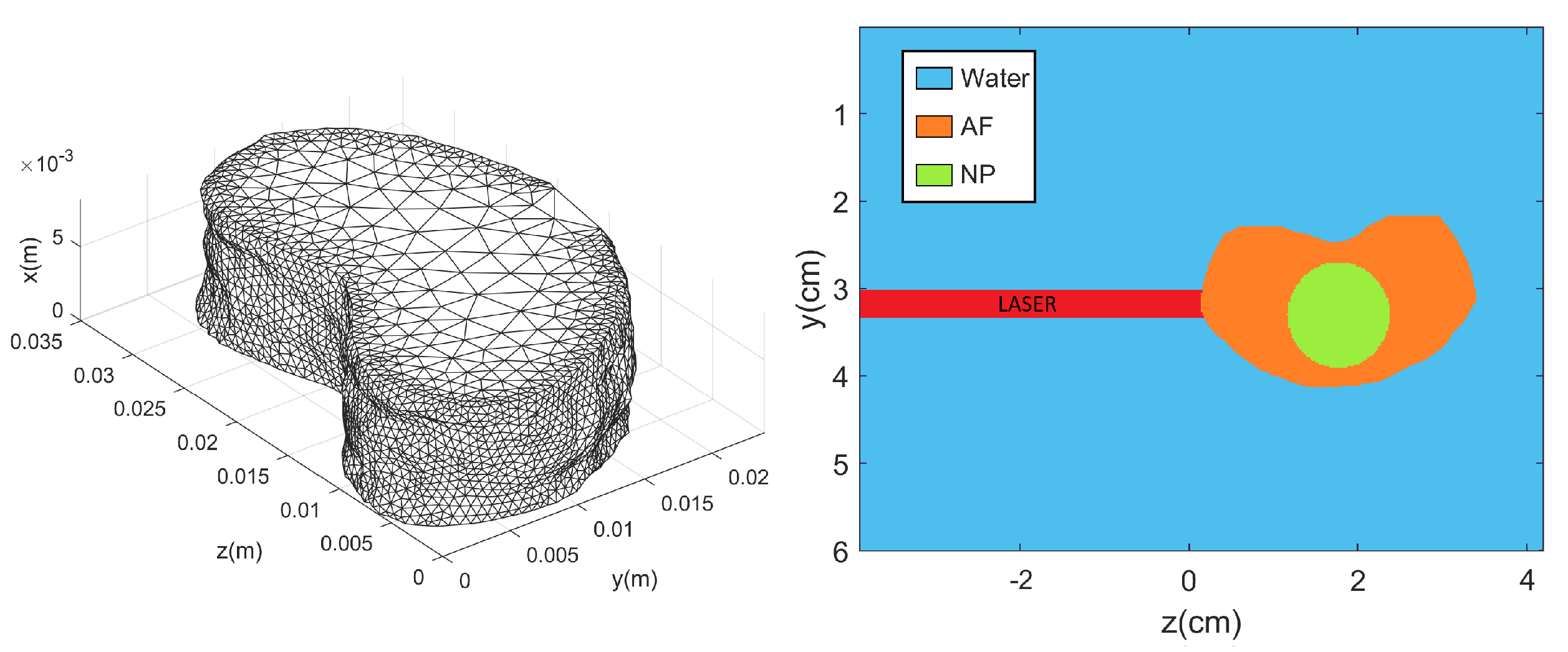
4. Building the Numerical Phantom
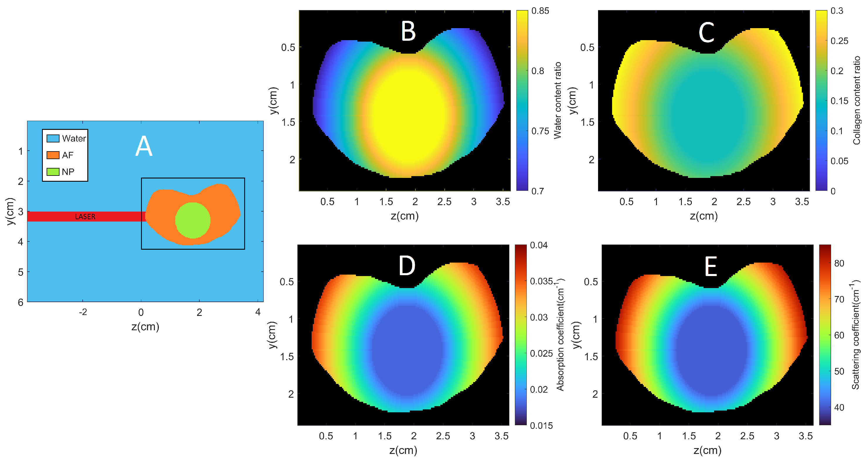
4.1. Defining the Morphology and Optical Properties
The morphology of the IVD was obtained from proton density-weighted MRI imaging of the IVD of a 4 month old pig taken from [11,12] (see Figure 2). The imaged disc was approximately 0.8 cm × 2.5 cm × 3.5 cm. The 3D morphology was integrated in a 512 × 512 × 512 voxel grid in MATLAB. The reconstructions were performed on a different grid of size 256 × 256 × 256 voxels to avoid the inverse crime. The surrounding medium was set to be water to fulfil the impedance matching condition needed for PA imaging. The spatial resolution in each direction was set to 0.02 cm. We differentiated the NP from the AF by modelling the NP as a simple cylinder at the centre of the disc, as presented in Figure 2. The laser illumination configuration used is presented in the same figure. The laser radius was 1.5 mm and the wavelength used was 532 nm. The laser radius was chosen based on the reference [10], where a similar beam radius was used (2 mm radius). The wavelength 532 nm was chosen because of the great difference of the absorption coefficients of collagen and water at this wavelength. This choice was also practical as it is a very common laser wavelength (e.g., Nd:YAG laser doubled in frequency with a KDP crystal).
Figure 2.
Morphology of the intervertebral disc (IVD): magnetic resonance imaging of a pig’s IVD (left) that was used to define the geometry in MATLAB (right), where the annulus fibrosus (AF) and nucleus pulposus (NP) are differentiated.
This simplified disc is made up of collagen and water only. The spatial changes in their proportion were taken into account and are presented in Figure 3. We set the proportion of collagen to linearly increase from 15% to 30% in the AF and the proportion of water in this zone to drop linearly from 85% to 70%. In the NP, the water and collagen proportions were supposed to be constant and equal to 85% and 15% respectively.
Figure 3.
Geometry of the numerical model (A). The area used is symbolized by the black rectangle. Proportions of water (B) and collagen (C) in the numerical IVD, and the associated absorption coefficient (D) and scattering coefficient (E).
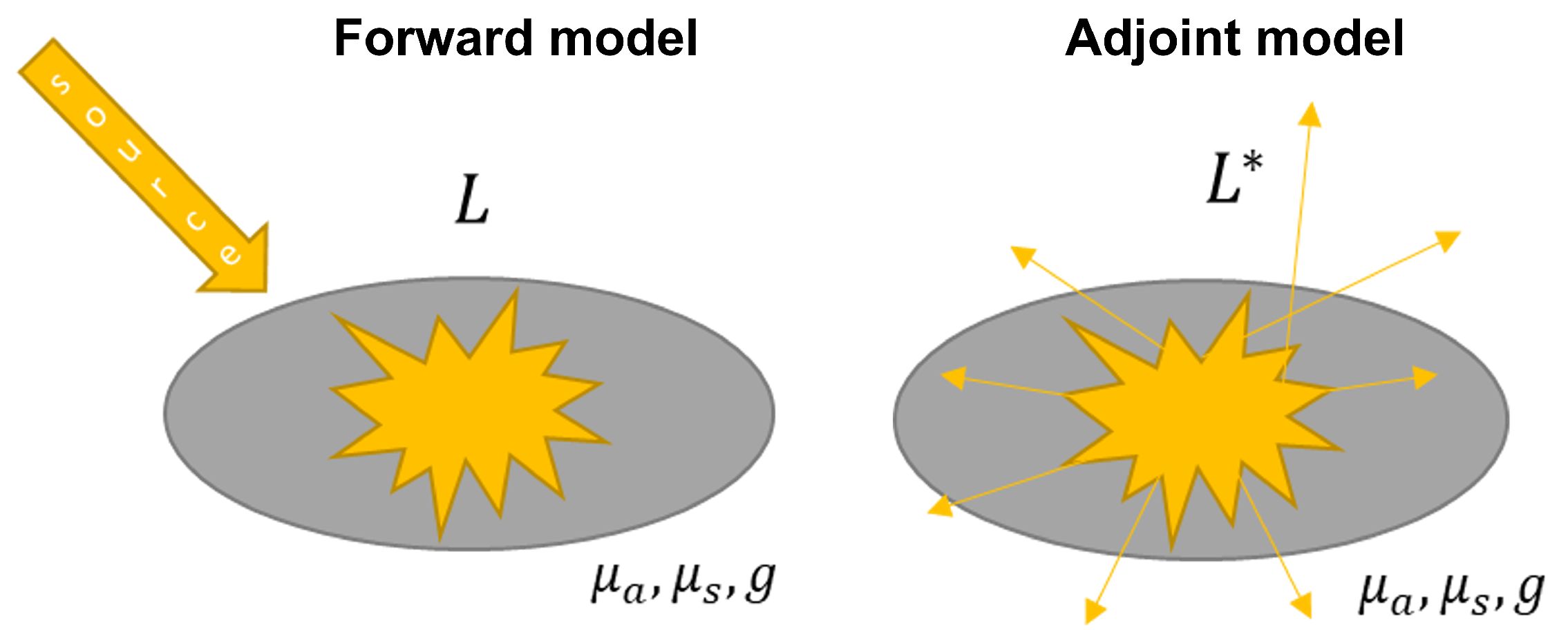
4.2. Gradient Descent Scheme
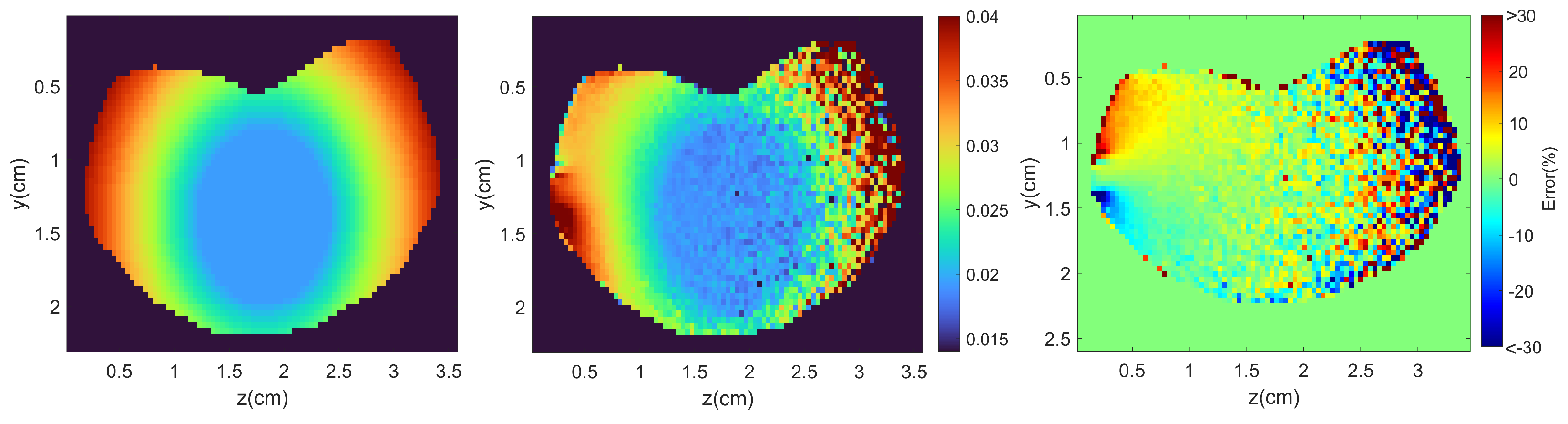
The QPAI inverse problem is based on an optimisation problem that aims at minimising an error function . In the scope of the optical inverse problem, this function is given as [9]:
corresponds to the synthetic measurements. It was calculated by Monte Carlo simulations with 3.10 photons here and presented in Figure 4.
Figure 4.
Top: Measurements of used for the reconstructions of the absorption coefficient (left). The right panel shows the measurements in log scale. The bottom graphs show the profile along the z-axis at the centre of the grid in non-log (left) and log (right) scales.
One can already note from such measurements that it will be difficult to recover optical properties deep in the IVD (right side) as the value of the absorbed optical energy H is very low in these areas. To have access to the entire disc, at least one other peripheric measurement has to be performed.
The gradient descent scheme requires the computation of the gradients of the error function with respect to the parameters of interest. The gradient with respect to the absorption coefficient can be written as [9]:
where L and are the radiance in W·m·sr and the adjoint radiance in W·m·sr, respectively. is the unit sphere. Note that these two parameters do not share the same units. The radiance L is the solution to the radiative transfer equation, and the adjoint radiance is the solution to its adjoint counterpart. In the forward problem, the source is the laser used. In the adjoint problem, the adjoint source is defined as:
which represents the difference between the measured and the modelled absorbed energy density. In this case, the source is the medium itself, emitting photons isotropically at each position where the difference is non-zero. Figure 5 presents schematic representations of the forward and adjoint problems.
Figure 5.
(Left): forward model where the source of light is the laser. (Right): adjoint model where the source is defined as the difference between the measure and the modelled absorbed energy density H.
To compute the gradient from Equation (6), we need the radiance in both the forward and adjoint models. Most Monte Carlo simulation softwares only offer the calculation of the fluence , which corresponds to the radiance integrated over all angles. In order to compute the radiance, the decomposition of the radiance into spherical harmonics (SH) was chosen:
where is the SH of order m and degree l, and are the corresponding coefficients. Using this decomposition in Equation (6) allows us to simplify the expression, as the SH form an orthonormal basis. The second term in Equation (6) can therefore be expressed as:
The simplified expression of the gradient using this decomposition is:
where corresponds to the SH coefficients of the adjoint radiance . The decomposition in SH implies the use of an infinite sum, but because of the finite computation time and memory, we stopped the decomposition at the degree of SH l = 3. The radiances L and were calculated by modifying MCmatlab and using the SH decomposition. The photons’ directional information (which was not stored in the original code) was taken into account by using the SH: the radiance is computed by storing the weight of photons going through the voxel at position r in the corresponding SH .
The gradient descent scheme step size was chosen to be that of the Barzilai–Borwein step [20]. This step size was chosen because it offers a great improvement in terms of rate of convergence compared to classical descent methods. We defined the step as spatially-varying: for each voxel defining the IVD geometry, a specific step size was calculated. To summarise, at the i-th iteration and at position r, the step size was computed as:
with and .
5. Results
Reconstructions of the absorption coefficient when the scattering coefficient was known were performed in three different situations: (i) by considering a perfect measurement (without any noise); (ii) in the same situation but without considering the radiance term in the gradient definition in Equation (6); (iii) when Gaussian noise was added to the measurement to test the robustness of the algorithm. 10 photons were simulated for all reconstructions for both the forward and adjoint radiance calculations. The gradient descent was initiated by setting a homogeneous absorption coefficient of 0.01 cm in the disc, which corresponds to an underestimated value. Negative and infinite absorption were not allowed in the algorithm. When one of these two cases was encountered in a voxel, the absorption coefficient of this voxel was set to the initial (0.01 cm). The optimisation algorithms were all stopped after 50 iterations, when no significant improvements of the reconstruction were seen. No regularisation methods were used in the following reconstructions.
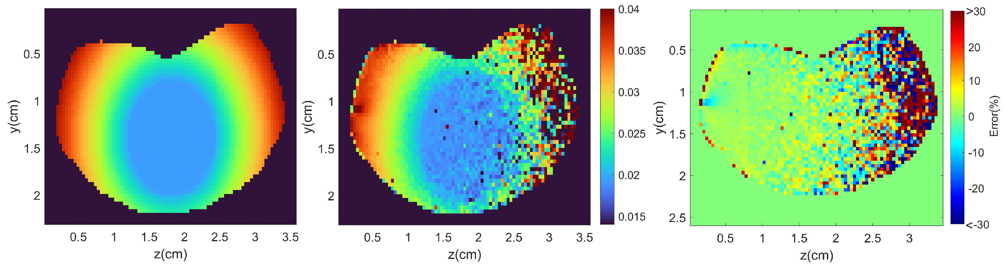
5.1. Noise-Free Reconstruction
Reconstruction of the spatially varying absorption coefficient with a noise-free measurement is presented in Figure 6.
Figure 6.
Target absorption coefficient (left). Reconstruction of the absorption coefficient (centre) with noise-free measurement after 50 iterations. Error percentage (right).
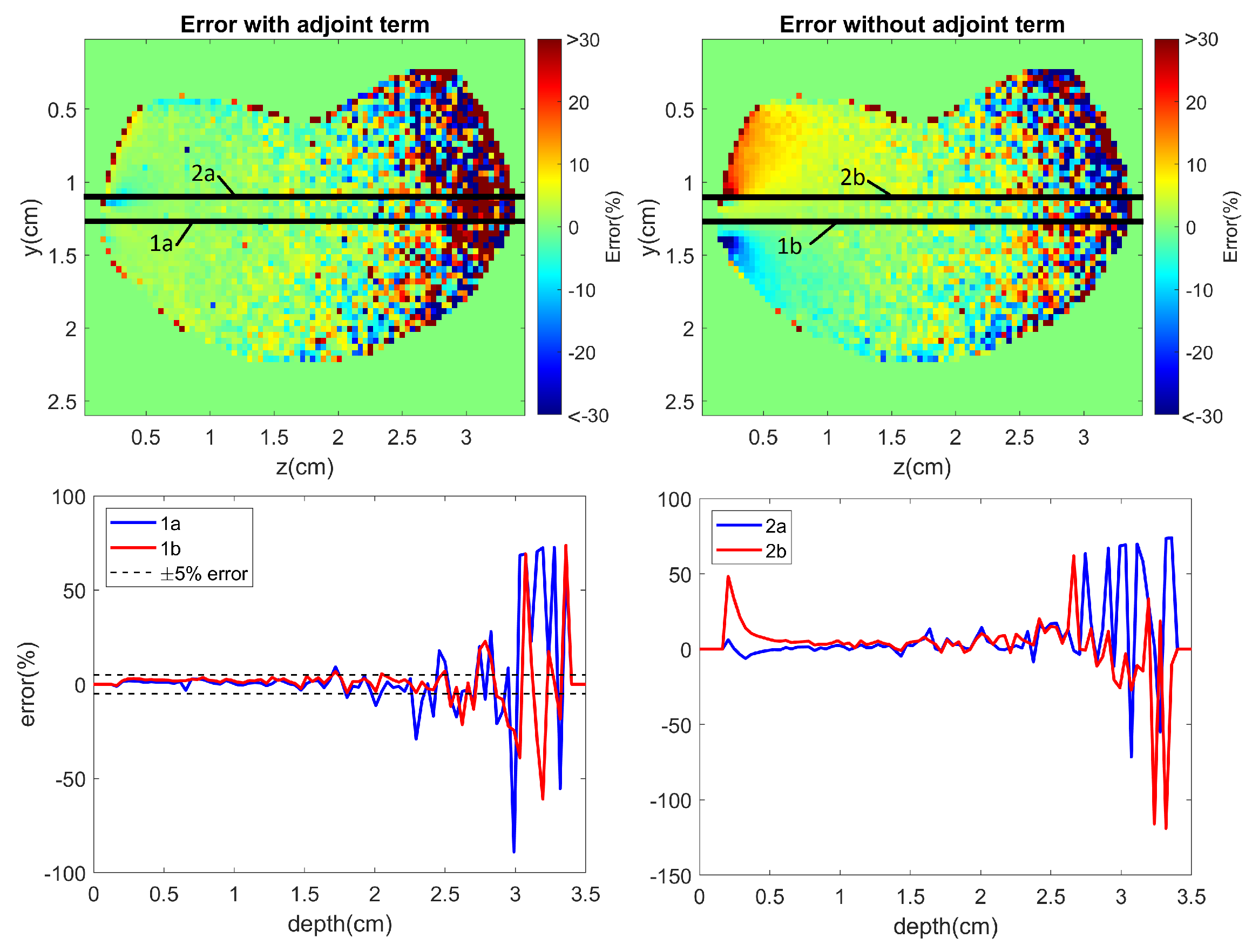
5.2. Reconstruction without the Radiance Term
When the scattering coefficient is constant in the medium, the second term in Equation (9) has been shown not to be necessary for an accurate reconstruction of the optical parameters [10]. In the IVD case, the scattering coefficient is not homogeneous and presents smooth spatial changes. To understand the contribution of this term containing the radiances to the reconstruction’s accuracy, a reconstruction without considering this radiance term was computed and compared to the case with the use of this term. In order to highlight its influence, a reconstruction without the radiance term is presented in Figure 7. A noise-free measurement was used.
Figure 7.
Target absorption coefficient (left). Reconstruction of the absorption coefficient (centre) with omitted radiance term after 50 iterations. Error percentage (right).
To compare the reconstructions with and without the radiance term, one-dimensional profiles of the error along the z-axis are presented in Figure 8.
Figure 8.
(Top): Representations of the chosen one-dimensional error profiles along the z-axis. (Bottom): Comparisons of the profiles with and without the radiance term: profiles 1a and 1b on the left and profiles 2a and 2b on the right.
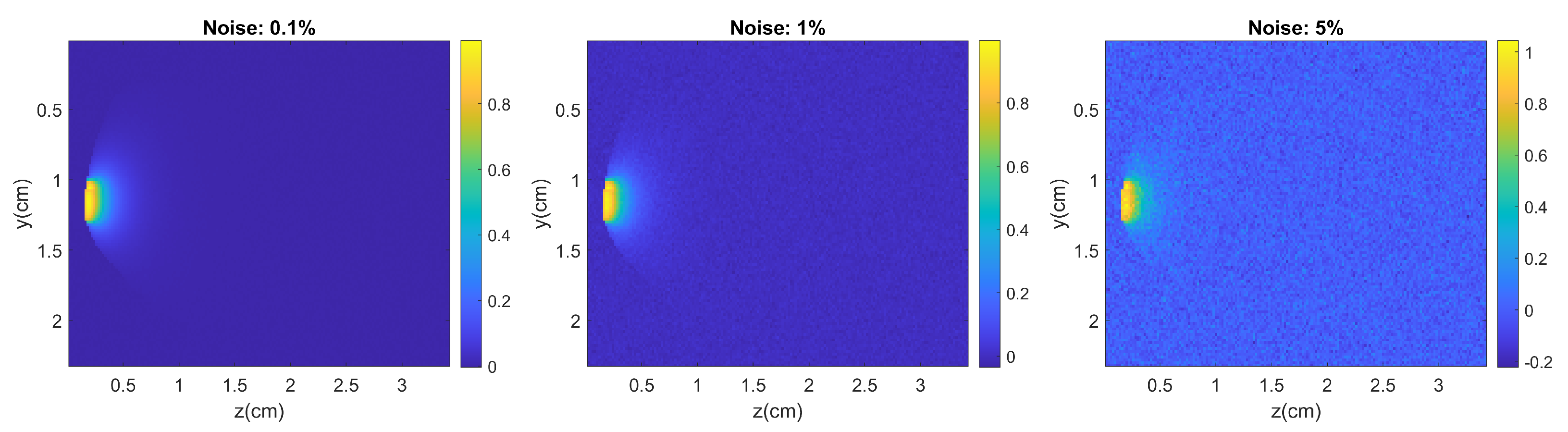
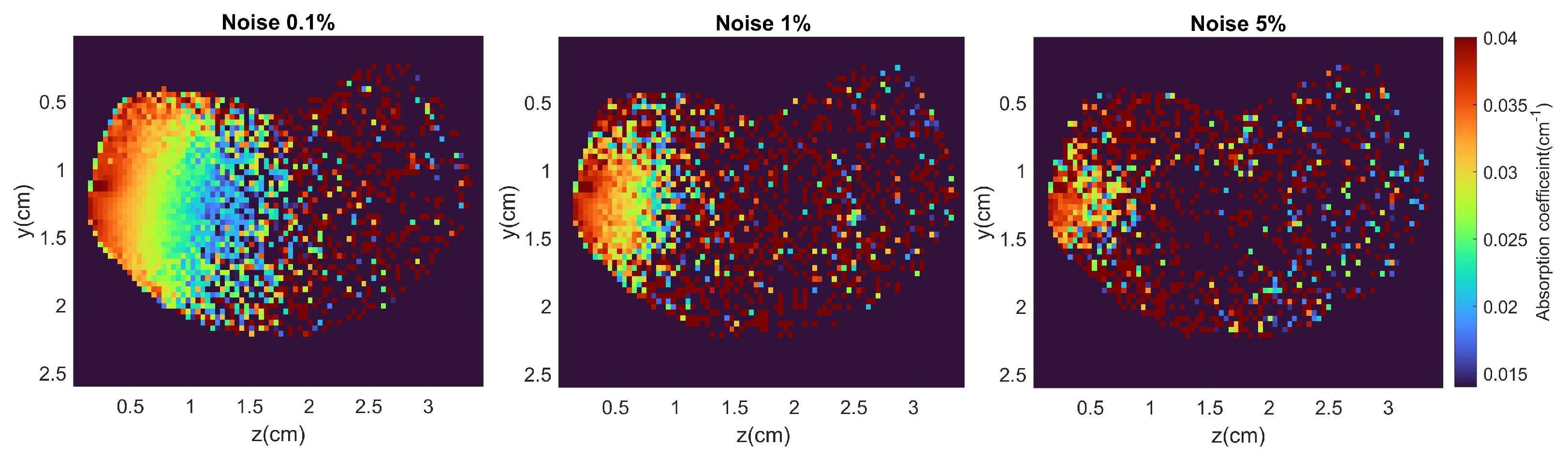
5.3. Reconstruction with Added Noise
Finally, a standard Gaussian noise ( = 1, = 0) was added to the measurement . The noise was added as a percentage of the maximum intensity of . Different percentages were chosen based on the noise levels reported in the literature [8,9,10,17,21]: three different percentages were considered: 0.1%, 1% and 5% of the maximum intensity of the measurement (see Figure 9).
Figure 9.
Measurements of with added noise. (Left) 0.1% noise; (centre) 1% noise; (right) 5% noise.
Results are presented in Figure 10.
Figure 10.
Noise’s effect on the reconstructions. (Left) 0.1% noise; (centre) 1% noise; (right) 5% noise.
6. Discussion
The results presented in Figure 6 show good agreement with target values of the absorption coefficient up to a limited depth that reaches the NP: in this noise-free reconstruction, the absorption coefficient was recovered with less than error up to a depth of approximately 1.5 cm (see Figure 8). The volume close to the laser illumination naturally yielded better results than deeper volumes due to the Monte Carlo simulation’s lower accuracy and the low values of the fluence. It is therefore not possible with the current configuration to obtain accurate reconstructions of the optical properties too deeply in a disc. It is clear that multiple measurements with multiple sources of illumination can improve the reconstruction in deeper areas. However, the goal here was to evaluate the feasibility of such measurement in the most simple, although constrained, acquisition geometry, keeping in mind that more complex measurements might be required to obtain satisfying reconstructions.
By comparing results in Figure 6 and Figure 7, the influence of the radiance term can be clearly seen near the illuminated surface of the IVD: the percentage of error is stronger in this volume. As can be seen in Figure 8, the reconstruction near this illuminated volume was performed with high error (approximately 50% error). With the radiance term, the error in this same volume was much lower (below 5%). This radiance term is therefore of particular importance when accurate quantification is required in superficial volumes.
Unsurprisingly, the reconstructions with added noise were degraded. The measurement of the absorbed energy density is important near the illuminated surface of the IVD, as can be seen in Figure 4. As one goes deeper into the IVD, this energy decreases until it reaches very low values. The added noise in this area is stronger than the significant value of the deposited energy, leading to highly inaccurate reconstructions. The stronger the noise intensity, the smaller the well-reconstructed volume is (Figure 10). This highlights the necessity of adding more information by multiplying the measurements, using an appropriate regularisation method or including prior knowledge to improve the results.
7. Conclusions
We conducted a preliminary study on the feasibility of using PA imaging to diagnose the viability of an IVD by accessing its relative water/collagen content through the reconstruction of the absorption coefficient with multispectral measurements. Reconstructions of the absorption coefficient at a given wavelength when the scattering coefficient was known were performed on a realistic digital phantom of an IVD of a pig obtained via MRI. Results show good agreement with the target absorption coefficient. The study shows the influence of the radiance term on the reconstruction when the scattering coefficient is heterogeneous. The low signal-to-noise ratio, however, is a challenge that needs to be solved in order to use this method for IVD probing. Prior knowledge, multiple illumination measurements or appropriate regularisation methods would improve the results and will be investigated in future works. The present study nonetheless showed encouraging results toward the use of PA for assessing the state of an IVD. Further works will also focus on the reconstruction of the scattering coefficient. More accurate representations of the disc morphology and composition (with proteoglycans content) will also be investigated. It is important to note that the present study did not address some limitations of QPAI: we did not consider problems related to the acoustic inverse problem, such as the limited bandwidth of the detectors. As we mentioned previously, we focused solely on the optical inverse problem. However, the acoustic inverse problem is fully addressed in the literature and will be tackled for IVDs in future works.
Author Contributions
Conceptualization, A.C.; methodology, A.C. and J.W; software, A.C. and J.W.; validation, R.A., O.B. and A.D.S.; formal analysis, A.C.; investigation, A.C.; resources, A.C. and M.G.; data curation, A.C.; writing—original draft preparation, A.C.; writing—review and editing, A.C., J.W., R.A., M.G., O.B. and A.D.S.; visualization, A.C.; supervision, O.B. and A.D.S.; project administration, A.D.S.; All authors have read and agreed to the published version of the manuscript.
Funding
This research received no external funding.
Institutional Review Board Statement
Not applicable.
Informed Consent Statement
Not applicable.
Data Availability Statement
Not applicable.
Conflicts of Interest
The authors declare no conflict of interest.
References
- Newell, N.; Little, J.; Christou, A.; Adams, M.; Adam, C.; Masouros, S. Biomechanics of the human intervertebral disc: A review of testing techniques and results. J. Mech. Behav. Biomed. Mater. 2017, 69, 420–434. [Google Scholar] [CrossRef] [PubMed]
- Kos, N.; Gradisnik, L.; Velnar, T. A Brief Review of the Degenerative Intervertebral Disc Disease. Med. Arch. 2019, 73, 421. [Google Scholar] [CrossRef] [PubMed]
- Katz, J.N. Lumbar Disc Disorders and Low-Back Pain: Socioeconomic Factors and Consequences. J. Bone Jt. Surg. 2006, 88, 21–24. [Google Scholar] [CrossRef]
- Lee, C.K. Accelerated Degeneration of the Segment Adjacent to a Lumbar Fusion. Spine 1988, 13, 375–377. [Google Scholar] [CrossRef] [PubMed]
- Tang, G.; Zhou, B.; Li, F.; Wang, W.; Liu, Y.; Wang, X.; Liu, C.; Ye, X. Advances of Naturally Derived and Synthetic Hydrogels for Intervertebral Disk Regeneration. Front. Bioeng. Biotechnol. 2020, 8, 745. [Google Scholar] [CrossRef] [PubMed]
- Yu, L.P.; Qian, W.W.; Yin, G.Y.; Ren, Y.X.; Hu, Z.Y. MRI Assessment of Lumbar Intervertebral Disc Degeneration with Lumbar Degenerative Disease Using the Pfirrmann Grading Systems. PLoS ONE 2012, 7, e48074. [Google Scholar] [CrossRef] [PubMed]
- Metwally, K.; Boiron, O.; Deplano, V.; Prost, S.; Da Silva, A. Probing intervertebral discs with photoacoustics. In Opto-Acoustic Methods and Applications in Biophotonics IV; Ntziachristos, V., Zemp, R., Eds.; SPIE: Munich, Germany, 2019; p. 61. [Google Scholar] [CrossRef]
- Cox, B.T.; Arridge, S.R.; Beard, P.C. Gradient-based quantitative photoacoustic image reconstruction for molecular imaging. In Photons Plus Ultrasound: Imaging and Sensing 2007: The Eighth Conference on Biomedical Thermoacoustics, Optoacoustics, and Acousto-Optics; Oraevsky, A.A., Wang, L.V., Eds.; International Society for Optics and Photonics, SPIE: Munich, Germany, 2007; Volume 6437, pp. 445–454. [Google Scholar] [CrossRef]
- Hochuli, R.; Powell, S.; Arridge, S.; Cox, B. Quantitative photoacoustic tomography using forward and adjoint Monte Carlo models of radiance. J. Biomed. Opt. 2016, 21, 126004. [Google Scholar] [CrossRef] [PubMed]
- Buchmann, J.; Kaplan, B.A.; Powell, S.; Prohaska, S.; Laufer, J. Three-dimensional quantitative photoacoustic tomography using an adjoint radiance Monte Carlo model and gradient descent. J. Biomed. Opt. 2019, 24, 1. [Google Scholar] [CrossRef] [PubMed] [Green Version]
- Chetoui, M.A.; Boiron, O.; Ghiss, M.; Dogui, A.; Deplano, V. Assessment of intervertebral disc degeneration-related properties using finite element models based on ρH-weighted MRI data. Biomech. Model. Mechanobiol. 2019, 18, 17–28. [Google Scholar] [CrossRef] [PubMed]
- Ghiss, M.; Giannesini, B.; Tropiano, P.; Tourki, Z.; Boiron, O. Quantitative MRI water content mapping of porcine intervertebral disc during uniaxial compression. Comput. Methods Biomech. Biomed. Eng. 2016, 19, 1079–1088. [Google Scholar] [CrossRef] [PubMed]
- Antoniou, J.; Steffen, T.; Nelson, F.; Winterbottom, N.; Hollander, A.P.; Poole, R.A.; Aebi, M.; Alini, M. The human lumbar intervertebral disc: Evidence for changes in the biosynthesis and denaturation of the extracellular matrix with growth, maturation, ageing, and degeneration. J. Clin. Investig. 1996, 98, 996–1003. [Google Scholar] [CrossRef] [PubMed]
- Bhattacharjee, M.; Ghosh, S. Silk biomaterials for intervertebral disk (IVD) tissue engineering. In Silk Biomaterials for Tissue Engineering and Regenerative Medicine; Elsevier: London, UK, 2014; pp. 377–402. [Google Scholar] [CrossRef]
- Iatridis, J.C.; MacLean, J.J.; O’Brien, M.; Stokes, I.A.F. Measurements of Proteoglycan and Water Content Distribution in Human Lumbar Intervertebral Discs. Spine 2007, 32, 1493–1497. [Google Scholar] [CrossRef] [PubMed]
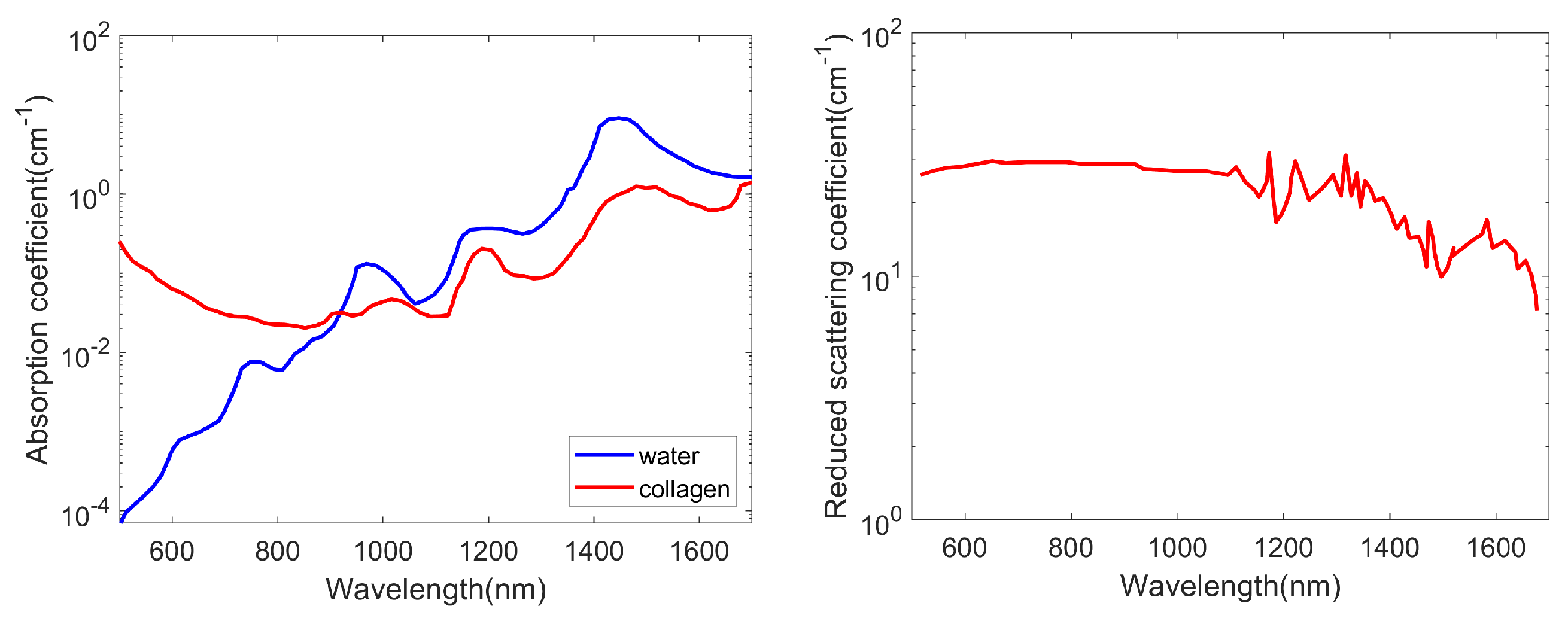
- Sekar, S.K.V.; Bargigia, I.; Mora, A.D.; Taroni, P.; Ruggeri, A.; Tosi, A.; Pifferi, A.; Farina, A. Diffuse optical characterization of collagen absorption from 500 to 1700 nm. J. Biomed. Opt. 2017, 22, 015006. [Google Scholar] [CrossRef] [PubMed] [Green Version]
- Mamonov, A.V.; Ren, K. Quantitative photoacoustic imaging in the radiative transport regime. Commun. Math. Sci. 2014, 12, 201–234. [Google Scholar] [CrossRef]
- Bal, G.; Ren, K. On multi-spectral quantitative photoacoustic tomography in diffusive regime. Inverse Probl. 2012, 28, 025010. [Google Scholar] [CrossRef]
- Marti, D.; Aasbjerg, R.N.; Andersen, P.E.; Hansen, A.K. MCmatlab: An open-source, user-friendly, MATLAB-integrated three-dimensional Monte Carlo light transport solver with heat diffusion and tissue damage. J. Biomed. Opt. 2018, 23, 1. [Google Scholar] [CrossRef] [PubMed]
- Barzilai, J.; Borwein, J.M. Two-Point Step Size Gradient Methods. IMA J. Numer. Anal. 1988, 8, 141–148. [Google Scholar] [CrossRef]
- Tarvainen, T.; Cox, B.T.; Kaipio, J.P.; Arridge, S.R. Reconstructing absorption and scattering distributions in quantitative photoacoustic tomography. Inverse Probl. 2012, 28, 084009. [Google Scholar] [CrossRef]
Publisher’s Note: MDPI stays neutral with regard to jurisdictional claims in published maps and institutional affiliations. |
© 2022 by the authors. Licensee MDPI, Basel, Switzerland. This article is an open access article distributed under the terms and conditions of the Creative Commons Attribution (CC BY) license (https://creativecommons.org/licenses/by/4.0/).


