Article

Magnetic Field Sensing Characteristics Based on Optical Microfiber Coupler Interferometer and Magnetic Fluid

1
Guangxi Key Laboratory of Multimedia Communications and Network Technology, School of Computer, Electronic and Information, Guangxi University, Nanning 530004, China
2
Center of Material Science, College of Liberal Arts and Sciences, National University of Defense Technology, Changsha 410073, China
3
State Key Laboratory of Transducer Technology, Shanghai Institute of Microsystem and Information Technology, Chinese Academy of Sciences, Shanghai 200050, China
*
Author to whom correspondence should be addressed.
Photonics 2021, 8(9), 364; https://doi.org/10.3390/photonics8090364
Submission received: 15 July 2021 / Revised: 24 August 2021 / Accepted: 28 August 2021 / Published: 30 August 2021
(This article belongs to the Special Issue Optical Sensing)

Abstract

:
In this paper, a novel and compact magnetic field sensor based on the combination of an optical microfiber coupler interferometer (OMCI) and magnetic fluid (MF) is proposed. The sensor is made up of an OMCI cover with polydimethylsiloxane (PDMS) and MF, and it uses MF as a material for adjusting the magnetic refractive index and magnetic field response. The sensing characteristics of the sensor are analyzed, and the experimental test is carried out. Under the condition of the same OMC waist length, the sensor sensitivity increases with the decrease of the OMC waist radius. The sensitivity of 54.71 and 48.21 pm/Oe was obtained when the OMC waist radius was set at 3.5 and 4 μm, respectively. In addition, we also tested the sensing response time and vector response characteristics of the sensor. At the same time, we discuss the demodulation idea about the cross-sensitivity of the magnetic field and temperature. The sensor has the advantages of high sensitivity, low cost, small size, optimized performance, and convenient integration. It has huge application potential in the fields of navigation and industrial intelligent manufacturing.

1. Introduction

The magnetic field sensor has important application value in navigation [1], military equipment application [2], biomedicine [3], and so on. With the development of ground vehicle detection [4,5], unexploded ordnance (UXO) detection [6,7], and unmanned aerial vehicles [8,9], new application requirements such as high sensitivity, high integration, wearable, low cost, miniaturization, and vector sensing are proposed for magnetic field sensors. Traditional magnetic field sensors are mostly based on electricity, and most of them have problems such as large volume, high cost, and weak anti-electromagnetic interference ability. Compared with traditional electrical magnetic field sensors, optical fiber magnetic field sensors have been widely studied due to the advantages of small size, low cost, convenient reuse, and easy integration [10].
At present, optical fiber magnetic field sensors can be divided based on the Faraday optical rotation effect [11,12], the magnetostrictive effect [13], and the refractive index control on MF [14,15,16] according to different sensing mechanisms. Among them, MF-based refractive index control sensors mainly use the light guide and magnetic response characteristics of the magnetic fluid to realize the magnetic field sensing function, and the optical field transmitted in the optical fiber is usually coupled with the magnetic fluid through a specific structure (this process is mainly realized by attenuating field coupling). In addition, the optical fiber magnetic field sensor with MF refractive index control has been widely studied because of its simple manufacturing and low cost. Depending on the fiber structure used, many structures of fiber have been proposed to make magnetic field sensors, and these structures include microfiber, fiber grating (FBG), photonic crystal fiber (PCF), etc. For example, Pu [14] developed the tapered fiber magnetic field sensor for the first time by combining the OMC-Sagnac ring with MF with a sensitivity of 19.4 pm/Oe, but the influence of the birefringence effect of the ring on the error of the response result was not considered. Moreover, the ring structure not only limits the sensor integration, but also the device is affected by temperature. Bao [15] made use of FBG and the Fabry–Perot (F-P) cavity structure combined with MF to fabricate a FBG-type magnetic field sensor, which obtained the magnetic field sensitivity of 2.42 pm/Oe; however, the realized sensitivity was too low. Li [16] used MF to fill the PCF hole and realized the magnetic field sensitivity of 0.072 nm/Gs in combination with the structure of the Mach–Zehnder interferometer, but the special fiber is expensive, and the production cost is high.
The evanescent field transmission fiber represented by OMC has a relatively large proportion of evanescent field transmission characteristics, and the transmitted light field will directly interact with the substance, which can greatly improve the sensitivity of the transmission fiber sensor.
Given this, we fabricated a new fiber-optic magnetic field sensor by combining OMC evanescent field transmission characteristics and magnetic fluid refractive index regulation characteristics. Under the theoretical guidance of the OMC coupling transmission principle and Michelson interferometer (MI) principle, two output ports of OMC were connected with Faraday rotation mirrors (FRM) to form an OMCI-MF structure. Compared with an FBG and PCF-integrated structure [15,16], the OMCI structure is vectorized and expands the integration performance of devices. At the interference arm region, we discussed the non-correlation of the interference arm to the magnetic field response and established the dual-parameter sensitivity matrix for the OMCI and MF refractive index control sensors. Compared with the traditional OMC-Sagnac ring [14] and OMC transmission structure [17], if the proposed sensor integrates temperature-sensitive or pressure-sensitive materials on the interference arm, it is expected to achieve multi-parameter sensing or temperature compensation performance based on magnetic field sensing. In addition, we verified the effect of the OMC radius on the magnetic field sensitivity through experiments. The proposed sensor has great application potential in national defense, medicine, marine applications, and so on.

2. Sensing Principle and Fabrication

2.1. Principle

The structure of the core optical component OMCI used in this sensor is shown in Figure 1. It was made by connecting two output ports of OMC with Faraday rotary mirrors. The OMC we used was made of two ordinary single-mode fibers fused and tapered. The OMCI consists of four ports, two transition regions, and a waist region.
According to the OMC coupling theory, Port 1 is adopted as the input port and Port 2 as the output port. The optical power (P3 and P4) reflected from Port 3 and Port 4 to the waist region can be respectively expressed as [18]:
P 3 = P 1 cos 2 ( C L )
P 4 = P 1 sin 2 ( C L )
where P1 is the input power of Port 1, L is the coupling length of the waist region, and C is the coupling coefficient. For the OMC with a melting taper, the coupling characteristics of the whole OMC in the uniform waist region play a leading role, and C can be respectively expressed as [17]:
C = 3 π λ 32 n 2 R 2 × 1 ( 1 + 1 / V ) 2
V = [ ( 2 π R ) / λ ] ( n 2 2 n 3 2 ) 1 2
In Formula (3) and (4), V is the normalized frequency, and λ represents the wavelength of the incident light, R represents the radius of OMC in the uniform waist region, n2 and n3 represent the refractive index of optical fiber cladding and MF, respectively. The output power (P2) of Port 2 can be expressed as [18]:
P 2 = 2 P 1 cos 2 ( C L ) sin 2 ( C L ) ( 1 + cos ( ϕ ) )
In Formula (5), ϕ = 2 π n 2 Δ l / λ represents the phase difference of the interference, Δ l = l 2 l 1 represents the arm difference of the interferometer. It can be seen that when n3 changes, the output power P2 also changes, which will cause the output spectrum to change, and the refractive index of the MF (n3) can be expressed by the Langevin model function as [19]:
n 3 ( H , T ) = [ n s n 0 ] [ coth ( α H H c , n T ) T α ( H H c , n ) ] + n 0
wherein ns is the saturation value of the refractive index, n0 is the initial refractive index of MF, α is the fitting coefficient, T is the temperature, Hc,n is the threshold domain. Due to the magneto-induced refractive index adjustability of MF, the characteristic wavelengths (dips or peaks) and reflection loss of the output spectrum will be sensitive to the external magnetic field. Therefore, the magnetic field can be measured by tracking the wavelength shifting and transmission loss of the output spectrum. For OMCI structure, because different arm differences will produce the phenomenon of change of interference fringe spacing in the envelope of each interference wave peak or interference wave trough, Δl should be controlled within 5–20 mm [18] to shape their envelope.

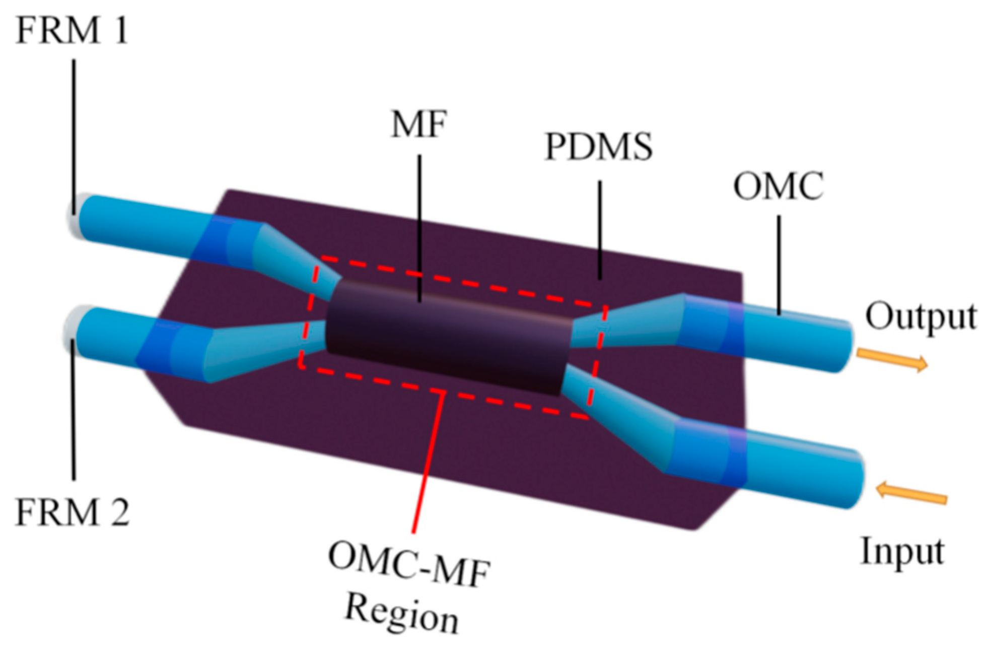
2.2. Structure and Fabrication

The structure of the sensor is shown in Figure 2, which mainly consists of two regions. In the OMC-MF region (the sensing region), the OMC transition regions and the waist regions covered by MF is encapsulated in a cuboid PDMS (104 × 8 × 12 mm) to effectively prevent air from entering the MF. The two interference arms of the sensor are of different lengths, and the two FRMs are connected to Port 3 and Port 4, respectively, so that the sensor is following the Michelson interferometer structure. In addition, compared with the ordinary coated mirror, the Faraday rotation mirror used by OMCI can reduce the polarization fading phenomenon caused by the birefringence effect of the single-mode fiber [20]. Stable interference waveforms can be observed intuitively on the output spectrum.
Before making the sensor, we designed a special metal bottom groove for the PDMS package model, which was used to make the U-shaped groove and sensor package based on PDMS, as shown in Figure 3a. First, we put the metal rod into the corresponding groove, and fixed the metal rod. Then we dropped the viscous PDMS into the groove. Note that the height of the gel liquid volume was parallel to the groove. We put it on a horizontal table for 20 min, and then we put it in the oven and heated it at 120 °C for 15 min. After heating, we cooled it for 5 min. After the PDMS was effectively cured, we carefully removed the metal rod to obtain a U-shaped groove as shown in Figure 3b.
We put the OMC finished products with melted tapering into the U-shaped groove. After sealing the two gaps of the U-shaped groove with PDMS liquid, we covered the U-shaped groove with pre-prepared PDMS sheets (about 1 mm thickness), as shown in Figure 3c. Then we put it in the oven and baked it at 120 °C for 15 min again [21]. After the PDMS was fully cured, we obtained the sensor probe sample without injection of the diluted MF, and the mixed MF liquid was injected into the PDMS void through a syringe. After the injection, vacuum tape was used to seal the injection hole. Finally, two Faraday rotary mirrors were connected to Port 3 and Port 4, respectively, and the sensor was finished as shown in Figure 3d. The sensor’s appearance is shown in Figure 3e.

3. Experiment Result

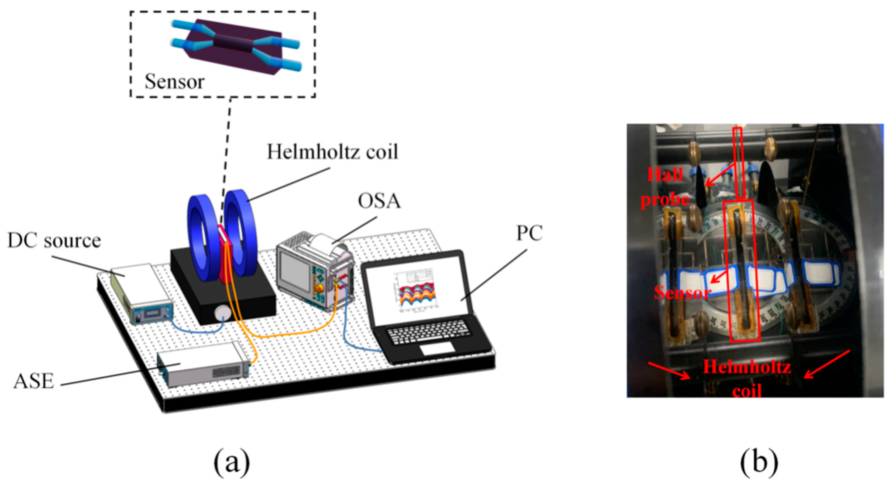
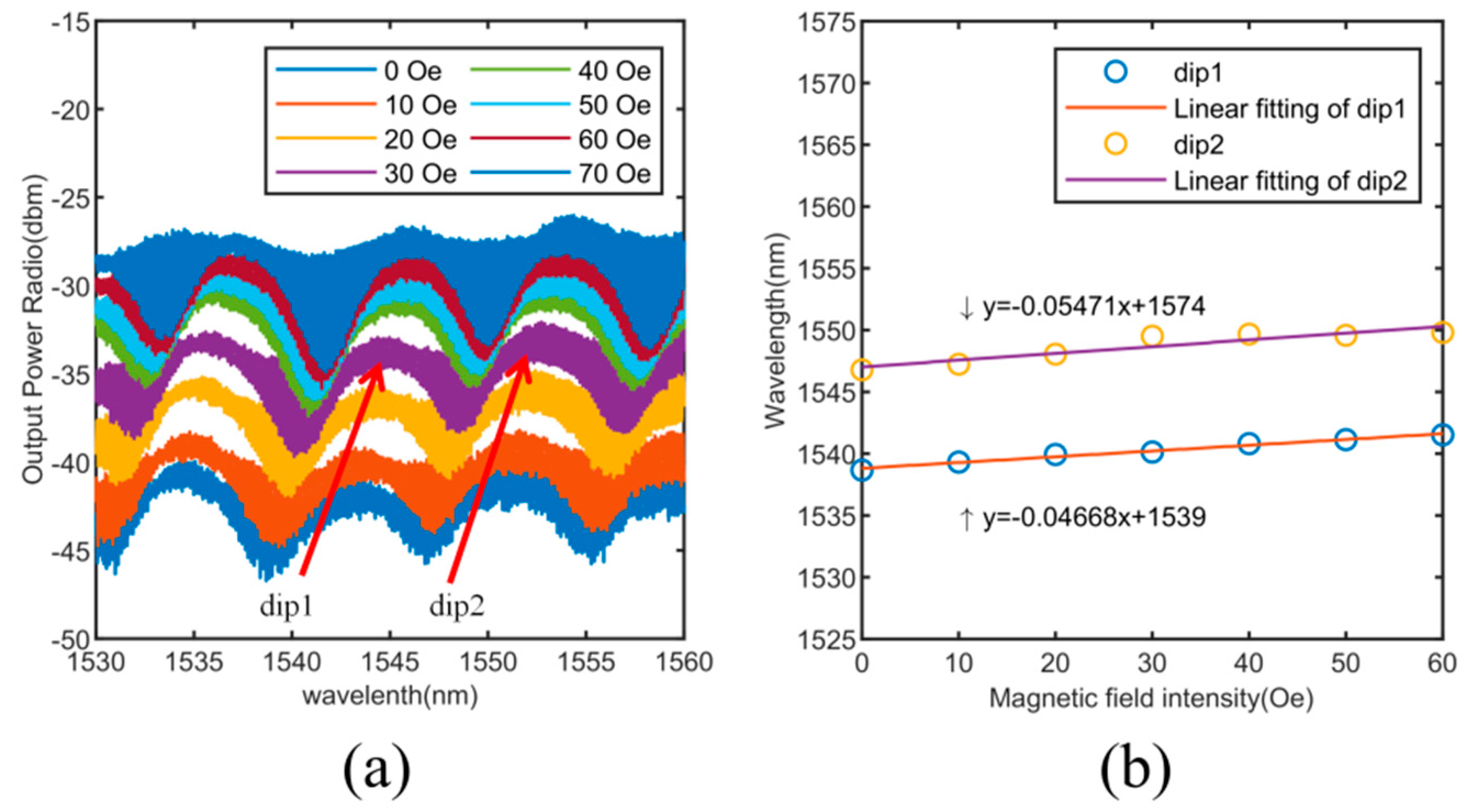
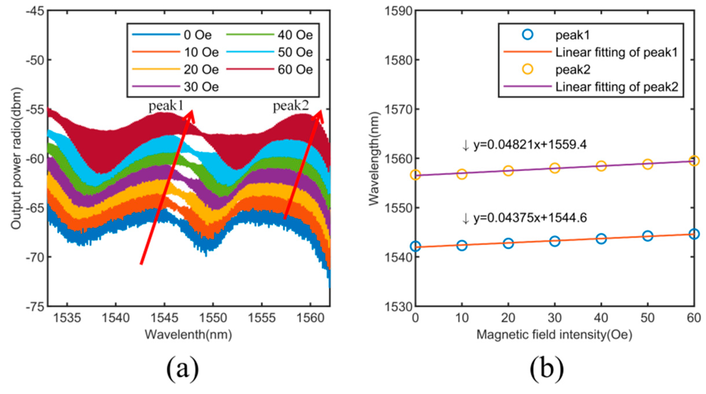
3.1. Magnetic Field Sensing Sensitivity Test

The setting of the magnetic field measurement system is shown in Figure 4. Input light from an amplified spontaneous emission (ASE, 1520~1620 nm) output was injected into the optical fiber via Port 1 and transmitted to an MF-filled OMCI sensor for the magnetic field. The programmable DC controls the power of the output current and generates a stable magnetic field through a set of Helmholtz coils. The reflected light was detected by the spectrometer (OSA, 600~1700 nm, Yokogawa, Japan, AQ6370D) through Port 2, and the data of the output spectrum were processed by a personal computer (PC).
First, sample 1 with the structural parameters of OMC as R of 3.5 μm and L of 9 mm was fabricated. We placed the sensor in the center of the coil and the initial arm difference of the interferometer was controlled as Δl ≈ 8 mm. The light travels through the sensor in a direction perpendicular to the magnetic field generated at the center of the coils. At the same time, to prevent FRMs from affecting the experimental results, FRMs were placed 3 m away from the Helmholtz coil. The magnetic field intensity was set to rise from 0 to 60 Oe, and the output spectrum was recorded every 10 Oe, and each recording interval was 10 min. The output spectrum of Port 2 was observed on OSA, as shown in Figure 5a. We used OSA to record the response spectrum (rapidly oscillating spectrum) of the sensor under a certain magnetic field intensity, and then used the “Peak Search” and “Bottom Search” functions of OSA to find these dips or peaks and record them. The spectral data derived from OSA were processed by MATLAB on the PC, which made it easy for us to filter and display the data in the form of images (including the setting of colors, line sizes, and axis values).
It can be seen from the result that the two characteristic wavelengths (dips) of the output spectrum redshift as the magnetic field increased. The refractive index of the magnetic fluid increases with the increase of the magnetic field [19] and the evanescent field generated in the OMC waist region was very sensitive to the change of refractive index around it, which leads to the dip shifts. Magnetic field sensitivity SB can be expressed as:
S B = Δ λ dip   or   peak Δ B
where ∆B is the changing magnetic field intensity and ∆λdip or peak is the drift of characteristic wavelength. Based on the above experimental results, we effectively realized the magnetic field sensing function of the sensor. According to the fitting curve in Figure 5b, the magnetic field sensitivity of the sample 1 is 46.68 pm/Oe for SB1-dip1 and 54.71 pm/Oe for SB1-dip2.
To verify the effect of OMC waist radius on sensitivity, sample 2 with the structural parameters of OMC as R of 4 μm and L of 9 mm was fabricated. In the experiment, the experimental testing process of sample 2 was the same as that of sample 1—between 0 and 60 Oe—and the obtained output spectrum is shown in Figure 6.
Similarly, by tracking the characteristic wavelengths (peak 1 and peak 2) in Figure 6a, we can see that they redshift as the magnetic field increases. According to the fitting curve in Figure 6b, the magnetic field sensitivity of sample 2 is 43.75 pm/Oe for SB2-peak1 and 48.21 pm/Oe for SB2-peak2.
In addition, we also estimated that the measurement resolutions of the sensors corresponding to sample 1 and sample 2 are approximately 0.183 and 0.207 Oe, respectively. It is worth noting that we found that the sensitivity of sample 1 is higher than that of sample 2. According to the theory of OMC evanescent field transmission [22], the smaller the uniform waist radius of OMC, the larger the proportion of evanescent field energy transmission. Compared with sample 2, the R of sample 1 is smaller (the L of the two samples is the same), so the OMC of sample 1 is more sensitive to changes in the refractive index around its uniform waist region, resulting in higher sensitivity of sample 1 (in the same magnetic field measurement range).

3.2. Test of Response Time
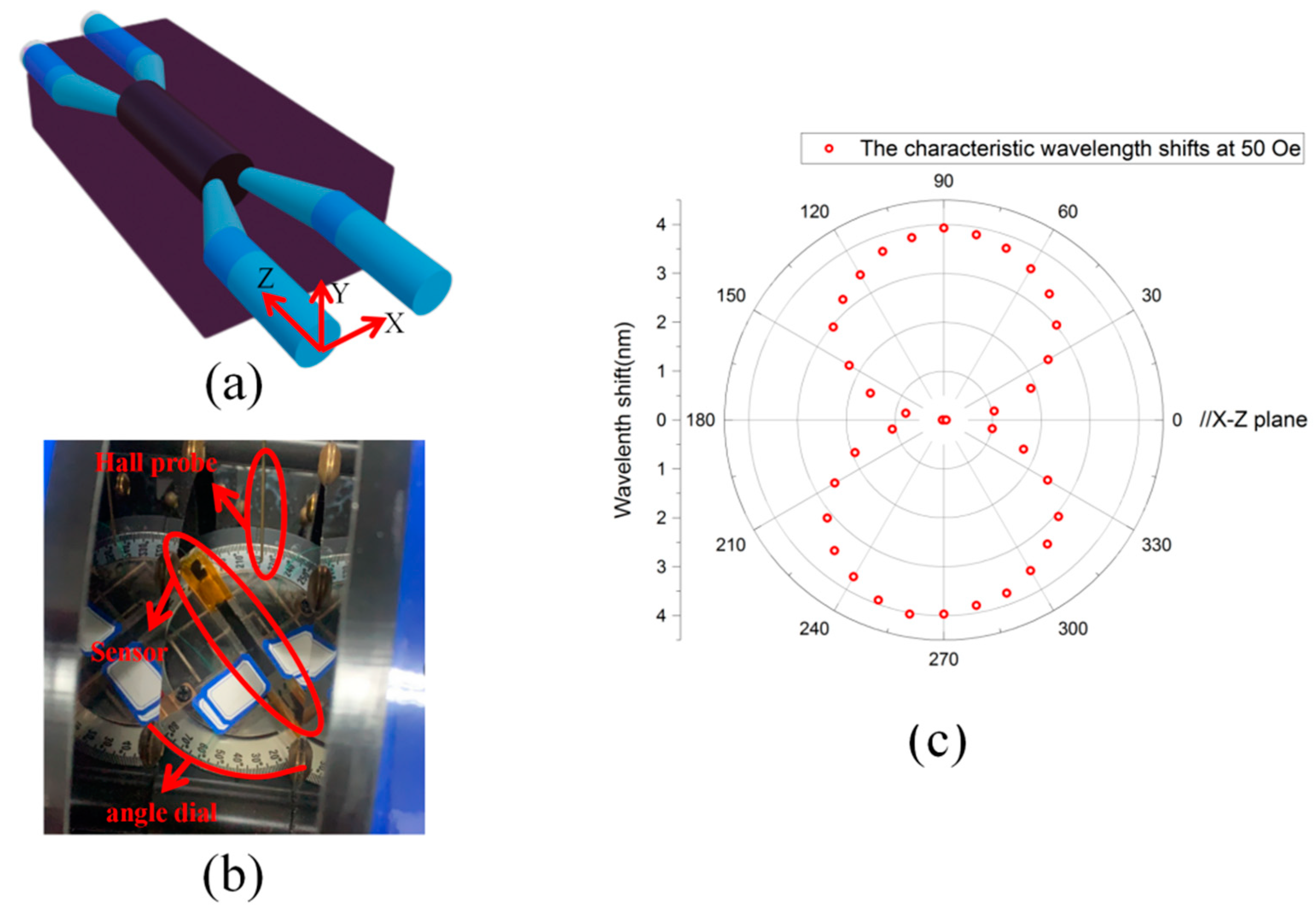
In addition, the response time of sample 1 was tested. The test system was mainly composed of a 1550 nm pumped laser source, a photodetector, a data acquisition card, a PC, a DC power supply, and a pair of Helmholtz coils.
The pumped laser source was injected through Port 1 of the fiber-optic sensor and Port 2 was connected with the photodetector. Then, the magnetic field strength was slowly increased to 60 Oe and was kept there for more than 10 min. The curve data of the magnetic field intensity and the voltage of the photodetector over time were recorded on the personal computer by the acquisition card. When the voltage reached a plateau at 60 Oe, we turned off the DC power supply, and the magnetic field dropped from 60 to 0 Oe quickly. Finally, after the voltage was stable, the time domain waveform of the whole test process was recorded, as shown in Figure 7. The response time of the sensor was measured to be 995 ms.

3.3. Test of Vector

Considering that the alignment direction of Fe3O4 nanoparticles in MF is different in different magnetic field directions, the refractive index around the uniform waist region of OMC will change accordingly [23]. To verify the influence of the direction of the magnetic field on the proposed sensor, sample 3 with the structural parameters of OMC as R of 4 μm and L of 9 mm was fabricated and the response of the sensor to the vector of the magnetic field at different angles in the X–Z plane was tested.
The sensor was placed under the magnetic field intensity of 50 Oe by rotating the angle dial at the center of the Helmholtz coil, as shown in Figure 8a,b. At 23.5 °C, we followed the shifts of characteristic wavelength and recorded its information every 10° at an interval of 5 min, and obtained the experimental results as shown in Figure 8c. We took the characteristic wavelength corresponding to 0° as the reference wavelength, and the positive direction of the Z-axis of the sensor was parallel to the 0° direction of the angle dial. It was found that under the action of different angles, the peak of the output spectrum drifts with the change of the magnetic vector, and the period of waveform drift was 90°. From 0° to 90°, the wavelength drift decreases and gradually approaches 0 with the increase of the angle. When the magnetic vector (0–90°) changes, the direction of the alignment chain of Fe3O4 nanoparticles around the OMC uniform waist region changes accordingly, thus affecting the refractive index around the OMC uniform waist region. Therefore, the output spectrum of the magnetic field response changes accordingly, indicating that the magnetic field sensor based on the OMC-MI refractive index control type was vectorizing compared with the OM-MF type [24].

4. Discussion

4.1. Influence of Interference Arm on Output Spectrum

Above, we have experimentally verified the response of the OMC-MF region of the sensor to the magnetic field, in which the interference arm and FRMs were not placed in the coil. To verify the influence of the interference arm on the output spectrum, sample 4 with the structural parameters of OMC as R of 3.5 μm and L of 9 mm was fabricated, and the sensor packaging process was the same as sample 1. Under the condition of 23.5 °C, we placed the two FRMs of the sensor in the center of the coils, gradually increased the magnetic field intensity from 0 to 40 Oe, and observed and recorded the output spectrum every 20 Oe interval. To prevent the influence of the OMC-MF region on the experimental results, we placed the OMC sensing region 3 m from the Helmholtz coil. The output spectrum of the sensor obtained in the experiment is shown in Figure 9a–c.
According to [18], the interference component assembly was used to make the sensor quasi-resonant, which can improve the sensitivity of the sensor and eliminate the polarization fading caused by the traditional OMC-Sagnac ring structure. In addition, the spacing of interference fringes within the interference envelope was also different according to the difference in arm difference. Formula (5) can be further decomposed into:
P 2 = 2 P 1 cos 2 ( C L ) sin 2 ( C L ) + 2 P 1 cos 2 ( C L ) sin 2 ( C L ) cos ( ϕ )
where 2 P 1 cos 2 ( C L ) sin 2 ( C L ) cos ( ϕ ) is the output power change caused by the round-trip phase delay of the interferometer. According to ϕ = 2 π n 2 Δ l / λ , we can see that the phase delay has the wavelength dependence and the arm difference (Δl) dependence. If the arm difference Δl is not 0, this is reflected in the interference fringes in the interference envelope of Figure 4, Figure 5, and Figure 9. On the contrary, if the arm difference Δl is 0, there will be no interference fringes in the interference envelope.
Figure 9a shows the output spectrum of the sensor at different magnetic field strengths when the interference arm is placed in the Helmholtz coil. We tracked the drift of dipB (1579.58 nm) in the magnified image. With the increase of magnetic field intensity, we found that the dipB did not drift. Meanwhile, the interference fringe spacing dB (the distance between dipB and its adjacent dip, dB = 0.1 nm) did not change, but there is a very small change in the output power, as shown in Figure 9b,c. Because we calibrated the sensitivity by tracking the drift of dipB, the small change of its output power did not affect the results of magnetic field measurement using the OMC-MF region.
The cause of output power changes under different magnetic fields may be the influence of ambient noise or background noise of the light source and OSA, or the effect of magnetic field on FRM may produce a small amount of polarization fading, but in general, the envelope of the output spectrum does not drift. Compared with the response result of the OMC-MF region to the magnetic field, the response result of FRM to the magnetic field can be ignored. Therefore, for the proposed sensor, the OMC-MF region plays a dominant role, while the FRMs act as a reflection device to shape the envelope of the output waveform.
The interference arm can be integrated with temperature-sensitive, pressure-sensitive, salt-sensitive, or humidity-sensitive expansion materials, which can be used to change the interference arm difference when the sensing parameters change so that the interference fringe spacing dB changes (but the change of dB may cause errors in magnetic field measurement). Therefore, the performance of multi-parameter sensing or parameter compensation correction (such as temperature compensation) can be achieved by changing the interference arm difference within the allowable error range.

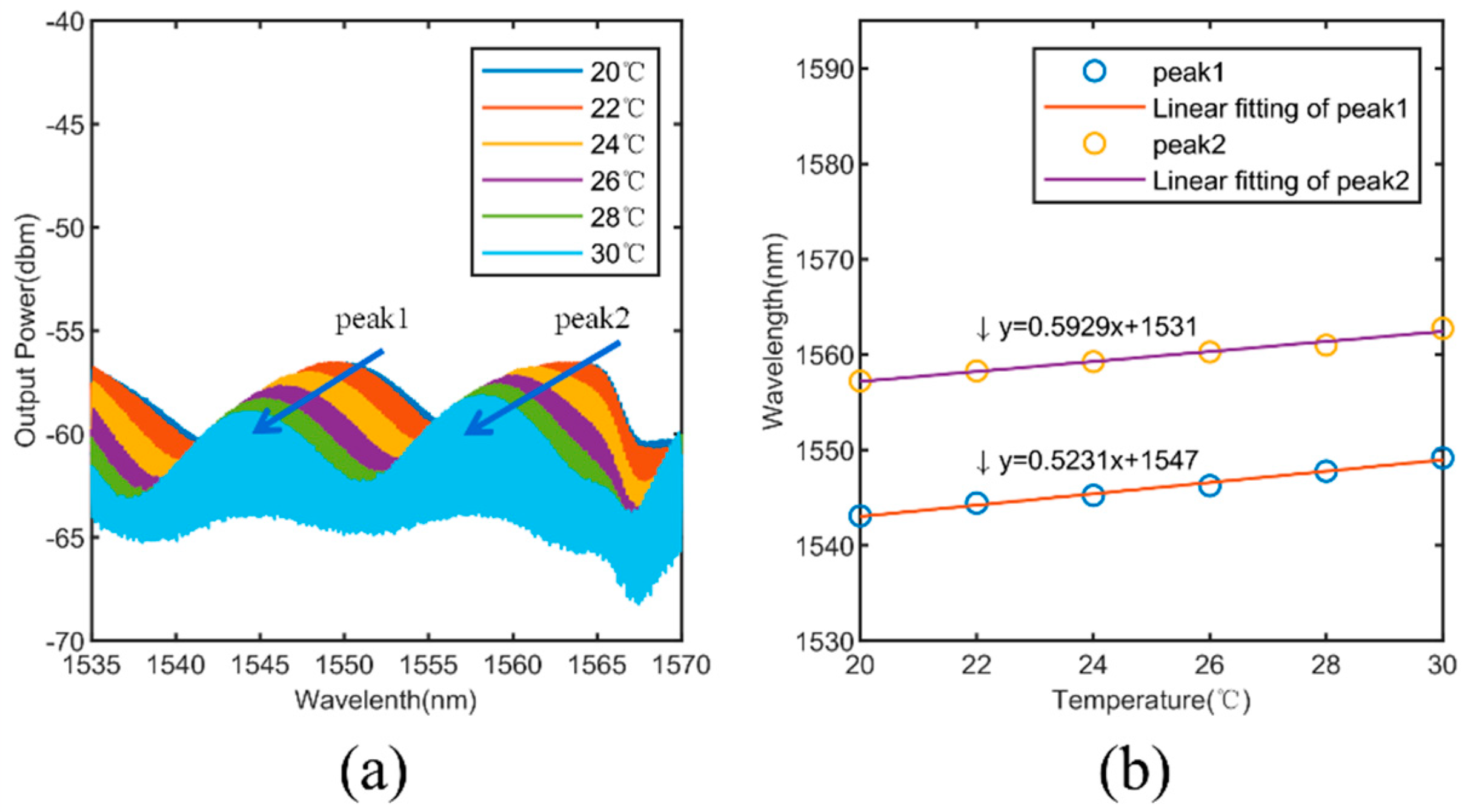
4.2. Dual-Parameter Demodulation

It can be seen from Equation (6) that the variation of the MF refractive index n3 is not only related to the size of the magnetic field but also related to the temperature. To verify the temperature response characteristics of the sensor, sample 4 with the structural parameters of OMC as R of 4 μm and L of 8 mm was fabricated. We put the sensor (sample 4) into the oven, and the temperature of the oven was increased from 20 to 30 °C, and the output spectrum was recorded at an interval of 2 °C. According to the fitting curve in Figure 6b, the temperature sensitivity of sample 4 is 523.1 pm/°C for ST1-peak1 and 592.9 pm/°C for ST1-peak2, as shown in Figure 10a,b.
Therefore, the change of temperature also causes the shift of the output spectrum, but the shift directions of the output spectrum for the temperature response and the magnetic field response is different. For one of our proposed sensors, if we calibrate its magnetic field sensitivity (SB1-Dip1 and SB1-Dip2) and temperature sensitivity (ST1-Dip1 and ST1-Dip2) respectively, a dual-parameter demodulation matrix can be established to demodulate ∆B and ∆T:
[ Δ λ d i p 1 Δ λ d i p 2 ] = [ S B 1 d i p 1 S T 1 d i p 1 S B 1 d i p 2 S T 1 d i p 2 ] [ Δ B Δ T ]
wherein the ∆λdip1 and the ∆λdip2 are the drift of dip1 and dip2. According to Equation (8), it can be observed that the characteristic of solving the matrix is that the output waveform of the sensor must generate more than two dips or peaks. Therefore, the difficulty in demodulating the matrix lies in the degree of mutual matching between magnetic field sensitivity and temperature sensitivity. Therefore, by making magnetic field sensors based on OMC-MF under different R values, we aim to optimize the magnetic field sensitivity of the sensor.
For the demodulation of the sensitivity matrix, the current data volume was not enough to demodulate the sensitivity matrix. Therefore, in the future, we will make different samples with different OMC sizes for the magnetic field and temperature response test, strive to demodulate and optimize the above sensitivity matrix, realize double-parameter demodulation or temperature compensation, and improve the demodulation accuracy.

5. Conclusions

In this paper, a new type of optical fiber magnetic field sensor based on OMCI was proposed. We have successfully carried out magnetic field experiments and theoretical verification. At the same time, we also verified the effect of the structural parameters of OMC (the radius of OMC) on the sensitivity change through different samples. The results show that the sensitivity of 54.71 and 48.21 pm/Oe was obtained when the OMC’s waist radius was set at 3.5 and 4 μm (under the same length of OMC’s waist), respectively. Compared with the traditional magnetic field sensors of OMC-Sagnac [14], OM-MF [24], and PCF-MF [16] structures, the advantages of the proposed sensor lie in its increased interference arm region. It is possible to integrate temperature-sensitive, pressure-sensitive, salt-sensitive, or humidity-sensitive materials into the interference arm of OMCI, which is of great significance for the realization of multi-parameter sensing or compensation performance, and the proposed sensor shows good vector property and time response.
The magnetic field sensor proposed in this paper has the advantages of high sensitivity, low cost, small volume, strong plasticity, and high integration, which is of great significance for wearable sensing, submarine pipeline detection, submarine resource exploration, biomedical sensing, and other aspects.

Author Contributions

Conceptualization, S.Q. and Y.Y.; Data curation, J.L. and M.L.; Formal analysis, S.Q.; Funding acquisition, Y.Y.; Project administration, Z.Z.; Supervision, Y.Y.; Writing—review and editing, S.Q., Y.Y., and J.Y. All authors have read and agreed to the published version of the manuscript.

Funding

This research was funded by National Natural Sciences Foundation of China (Grant Nos. 61805278); National Natural Science Foundation of China (Grant Nos. 61661004); The Guangxi Science Key Research and Development Project (Guangxi Science AB1850043); State Key Laboratory of Transducer Technology of China (No. SKT2001).

Institutional Review Board Statement

Not applicable.

Informed Consent Statement

Not applicable.

Data Availability Statement

Not applicable.

Acknowledgments

We thank the College of Liberal Arts and Sciences in the National University of Defense Technology for providing manufacturing equipment for OMC and testing the sensors, and thank the School of Computer, Electronics, and Information in Guangxi University for providing financial support for our research.

Conflicts of Interest

The authors declare no conflict of interest.

References

  1. Ilyas, M.; Cho, K.; Baeg, S.; Park, S. Drift Reduction in Pedestrian Navigation System by Exploiting Motion Constraints and Magnetic Field. Sensors 2016, 16, 1455. [Google Scholar] [CrossRef] [Green Version]
  2. Phan, M.; Peng, H. Giant magnetoimpedance materials: Fundamentals and applications. Prog. Mater. Sci 2008, 53, 323–420. [Google Scholar] [CrossRef]
  3. Murzin, D.; Mapps, D.J.; Levada, K.; Belyaev, V.; Omelyanchik, A.; Panina, L.; Rodionova, V. Ultrasensitive Magnetic Field Sensors for Biomedical Applications. Sensors 2020, 20, 1569. [Google Scholar] [CrossRef] [PubMed] [Green Version]
  4. Wang, Q.; Zheng, J.; Xu, H.; Xu, B.; Chen, R. Roadside Magnetic Sensor System for Vehicle Detection in Urban Environments. IEEE Trans. Intell. Transp. 2018, 19, 1365–1374. [Google Scholar] [CrossRef]
  5. Feng, Y.; Mao, G.; Cheng, B.; Li, C.; Hui, Y.; Xu, Z.; Chen, J. MagMonitor: Vehicle Speed Estimation and Vehicle Classification Through A Magnetic Sensor. IEEE Trans. Intell. Transp. 2020, 1–12. [Google Scholar] [CrossRef]
  6. Billings, S.; Beran, L. Optimizing electromagnetic sensors for unexploded ordnance detection. Geophysics 2017, 82, EN25–EN31. [Google Scholar] [CrossRef]
  7. Huang, H.; Won, I.J. Automated anomaly picking from broadband electromagnetic data in an unexploded ordnance (UXO) survey. Geophysics 2003, 68, 1870–1876. [Google Scholar] [CrossRef]
  8. Martinović, D.; Bogdan, S.; Kovačić, Z. Mathematical Considerations for Unmanned Aerial Vehicle Navigation in the Magnetic Field of Two Parallel Transmission Lines. Appl. Sci. 2021, 11, 3323. [Google Scholar] [CrossRef]
  9. Maire, P.L.; Bertrand, L.; Munschy, M.; Diraison, M.; Géraud, Y. Aerial magnetic mapping with a UAV and a fluxgate magnetometer: A new method for rapid mapping and upscaling from the field to regional scale. Geophys. Prospect. 2020, 68, 2307–2319. [Google Scholar] [CrossRef]
  10. Peng, J.; Jia, S.; Bian, J.; Zhang, S.; Liu, J.; Zhou, X. Recent Progress on Electromagnetic Field Measurement Based on Optical Sensors. Sensors 2019, 19, 2860. [Google Scholar] [CrossRef] [Green Version]
  11. Sun, L.; Jiang, S.; Marciante, J.R. All-fiber optical magnetic-field sensor based on Faraday rotation in highly terbium-doped fiber. Opt. Express 2010, 18, 5407–5412. [Google Scholar] [CrossRef] [PubMed]
  12. Amirsolaimani, B.; Gangopadhyay, P.; Persoons, A.P.; Showghi, S.A.; LaComb, L.J.; Norwood, R.A.; Peyghambarian, N. High sensitivity magnetometer using nanocomposite polymers with large magneto-optic response. Opt. Lett. 2018, 43, 4615–4618. [Google Scholar] [CrossRef]
  13. Davino, D.; Visone, C.; Ambrosino, C.; Campopiano, S.; Cusano, A.; Cutolo, A. Compensation of hysteresis in magnetic field sensors employing Fiber Bragg Grating and magneto-elastic materials. Sens. Actuators A Phys. 2008, 147, 127–136. [Google Scholar] [CrossRef]
  14. Pu, S.; Mao, L.; Yao, T.; Gu, J.; Lahoubi, M.; Zeng, X. Microfiber Coupling Structures for Magnetic Field Sensing With Enhanced Sensitivity. IEEE Sens. J. 2017, 17, 5857–5861. [Google Scholar] [CrossRef]
  15. Bao, L.; Dong, X.; Zhang, S.; Shen, C.; Shum, P.P. Magnetic Field Sensor Based on Magnetic Fluid-Infiltrated Phase-Shifted Fiber Bragg Grating. IEEE Sens. J. 2018, 18, 4008–4012. [Google Scholar] [CrossRef]
  16. Li, X.; Zhou, X.; Zhao, Y.; Lv, R. Multi-modes interferometer for magnetic field and temperature measurement using Photonic crystal fiber filled with magnetic fluid. Opt. Fiber Technol. 2018, 41, 1–6. [Google Scholar] [CrossRef]
  17. Luo, L.; Pu, S.; Tang, J.; Zeng, X.; Lahoubi, M. Highly sensitive magnetic field sensor based on microfiber coupler with magnetic fluid. Appl. Phys. Lett. 2015, 106, 193507. [Google Scholar] [CrossRef]
  18. Zhou, L.; Yu, Y.; Huang, H.; Tao, Y.; Wen, K.; Li, G.; Yang, J.; Zhang, Z. Salinity Sensing Characteristics Based on Optical Microfiber Coupler Interferometer. Photonics 2020, 7, 77. [Google Scholar] [CrossRef]
  19. Chen, Y.F.; Yang, S.Y.; Tse, W.S.; Horng, H.E.; Hong, C.; Yang, H.C. Thermal effect on the field-dependent refractive index of the magnetic fluid film. Appl. Phys. Lett. 2003, 82, 3481–3483. [Google Scholar] [CrossRef]
  20. Zhang, H.; Dong, Y.; Leeson, J.; Chen, L.; Bao, X. High sensitivity optical fiber current sensor based on polarization diversity and a Faraday rotation mirror cavity. Appl. Opt. 2011, 50, 924. [Google Scholar] [CrossRef] [PubMed]
  21. Hou, Y.; Wang, J.; Wang, X.; Liao, Y.; Yang, L.; Cai, E.; Wang, S. Simultaneous Measurement of Pressure and Temperature in Seawater with PDMS Sealed Microfiber Mach-Zehnder Interferometer. J. Lightw. Technol. 2020, 38, 6412–6421. [Google Scholar] [CrossRef]
  22. Tong, L.; Lou, J.; Mazur, E. Single-mode guiding properties of subwavelength-diameter silica and silicon wire waveguides. Opt. Express 2004, 12, 1025–1035. [Google Scholar] [CrossRef] [PubMed]
  23. Li, Y.; Pu, S.; Zhao, Y.; Zhang, R.; Jia, Z.; Yao, J.; Hao, Z.; Han, Z.; Li, D.; Li, X. All-fiber-optic vector magnetic field sensor based on side-polished fiber and magnetic fluid. Opt. Express 2019, 27, 35182. [Google Scholar] [CrossRef] [PubMed]
  24. Tian, H.; Song, Y.; Li, Y.; Li, H. Fiber-Optic Vector Magnetic Field Sensor Based on Mode Interference and Magnetic Fluid in a Two-Channel Tapered Structure. IEEE Photonics J. 2019, 11, 1–9. [Google Scholar] [CrossRef]
Figure 1. Structure of OMCI.
Photonics 08 00364 g001
Figure 2. The structure of the sensor.
Photonics 08 00364 g002
Figure 3. Sensor fabrication process. (a) Fabrication process of U-shaped groove. (b) U-shaped groove after cooling. (c) Place the OMC in the U-shaped groove. (d) Injection of magnetic fluid. (e) Picture of sensor appearance.
Photonics 08 00364 g003
Figure 4. (a) Diagram of magnetic field test system. (b) The sensor is placed in Helmholtz coils.
Photonics 08 00364 g004
Figure 5. (a) Sample 1: Output spectrums under a magnetic field range of 0-60 Oe. (b) Linear fitting of characteristic wavelength (dips) shifting for magnetic response.
Photonics 08 00364 g005
Figure 6. (a) Sample 2: Output spectrums under a magnetic field range of 0-60 Oe. (b) Linear fitting of characteristic wavelength (peaks) shifting for magnetic response.
Photonics 08 00364 g006
Figure 7. Response time of the sensor and Helmholtz coils from 60-0 Oe.
Photonics 08 00364 g007
Figure 8. (a) The sensor is placed in a Helmholtz coil with an angle dial. (b) The experiment measured the shifts of characteristic wavelength for different magnetic field vectors at 50 Oe. (c) Characteristic wavelength shifts when the rotation angle changed from 0° to 360° at 50 Oe in the X-Z plane.
Photonics 08 00364 g008
Figure 9. (a) The output spectrum of the sensor at different magnetic field strengths when the interference arm is placed in the Helmholtz coil. (b) Detailed diagram of interference fringe spacing dB. (c) Details of dipB.
Photonics 08 00364 g009
Figure 10. (a) Sample 4: Output spectrums under a temperature range of 20–30 °C. (b) Linear fitting of characteristic wavelength (peaks) shifting for temperature response.
Photonics 08 00364 g010
Publisher’s Note: MDPI stays neutral with regard to jurisdictional claims in published maps and institutional affiliations.

