Article

New Solutions of Laser-Induced Fluorescence for Oil Pollution Monitoring at Sea

1
Maritime State University named after Admiral G.I. Nevelskoy, Maritime Technopark, 690003 Vladivostok, Russia
2
Laboratory of Analytical Laser Spectroscopy, Far Eastern Federal University, 690091 Vladivostok, Russia
*
Author to whom correspondence should be addressed.
Photonics 2020, 7(2), 36; https://doi.org/10.3390/photonics7020036
Submission received: 21 April 2020 / Revised: 16 May 2020 / Accepted: 26 May 2020 / Published: 28 May 2020
(This article belongs to the Section Lasers, Light Sources and Sensors)

Abstract

:
Laser-induced fluorescence (LIF) spectral features for oil products of different states (solutions in the seawater and thin slicks) are discussed in this article. This research was done to evaluate LIF application for the identification of oil products and the measurement of the volume of ocean pollution by bilge water disposal. It was found out that the form of LIF spectral distribution was changed depending on the oil product state (pure fuel, slick or solution). The LIF method was calibrated for the most common types of heavy and light marine fuels at the standard measurement method of solution concentrations and limit of detection (LoD) values were established for each type. The time dynamics of the solution spectra were researched, and the time change features were determined. The smallsized LIF sensor for the unmanned aerial vehicle (UAV) is described and aims to investigate the LIF for oil pollution at sea.

Graphical Abstract

1. Introduction

Laser-induced fluorescence (LIF) is an informative method to research a matter [1,2,3]. Many scientists improve LIF to apply it for sea oil pollution monitoring. LIF application for oil spill monitoring at sea was studied for many years [4,5], but it still occurs [6,7,8,9]. The competitive analysis of available sensors for oil pollution at sea shows that LIF is one of the most enlightening and informative methods for oil spill monitoring [10]. It allows detecting the pollution and the recognition of the oil or oil products [11]. The volume of the pollution by oil products (thin slicks on the sea surface or solutions in the seawater) may be evaluated based on the LIF spectra analysis [12,13].
Nowadays, there are quite distinctive LIF spectrometers for oil spill monitoring by plane [14,15,16] or by vessel [17,18,19]. In some cases, LIF spectrometers were used not only as scientific equipment but also to obtain the information about the exact pollution [20].
However, the practice of using LIF spectra shows that airborne LIF spectrometers or its versions for the vessels may be beneficial only if it is applied for the specific research of big sea areas or offshore oil disasters. It is not efficient to use such equipment for everyday sea monitoring or oil spill monitoring at a regional scale [17,21].
It is crucial to improve LIF application due to increased pollution which is caused by illegal bilge water disposal, bunkering accidents and other accidents of small scale. Such pollution at the regional scale is becoming a dominating part of the total pollution of the World Ocean [22,23].
LIF and necessary equipment have been developed in the recent years for commercial unmanned aerial vehicles (UAV) [24,25]. Laser technologies, methods, the equipment of spectral analysis and spectral data processing, including methods of artificial intelligence, are being improved. Now it is possible to start the development and design of the monitoring equipment which is beneficial, prompt and easy to be serviced for small scale pollution. This research is aimed to solve the following tasks for LIF:
-
LIF development for the prompt measurement of concentrations of dissolved oil products in the seawater;
-
Development of the identification method of oil product type, which caused the pollution (slick and dissolved state), by machine learning.
The first task is explained by a substantial volume of pollution, which is caused by illegal bilge water disposal by vessels. Pollution by bilge water is a process when oil products of different concentrations enter the upper layer of the ocean. This process does not always cause the slick on the sea surface, and it depends on the concentration value of the oil hydrocarbon in the bilge water and hydrology parameters of the marine environment. The permissible concentration for dissolved oil hydrocarbons is 15 ppm, limited for bilge water disposal by vessels [26]. This concentration is quite a small, and this it is now essential to develop the prompt LIF method which can measure such small concentrations of oil hydrocarbons in the seawater.
The second aforementioned task may be solved within a broad scope of LIF. There are developed methods of identification for different types of oil products which are based on the analysis of distinct LIF spectra [24,27,28]. These methods are based on the analysis of distinctive features of the LIF spectra (maxima position, the intensity ratio of the chosen spectral bands or time-resolved fluorescence). Nonetheless, recognition methods of oil types by LIF spectra may be improved by methods of recognition which are based on machine learning. It is therefore crucial to collect data sets with the LIF spectra of solutions and slicks of the most common types of marine fuels. It is necessary to research the LIF spectral characteristics of oil products in different states such as thin slick on the sea surface or solution in the seawater. Such distinctive features of spectra should be defined for each type of oil product which are often noticed as pollutants of the ocean. Machine learning must include all of these distinctive features to recognize different types of oil products.
This research presents laboratory investigations of LIF spectra which may widen the scope of LIF application for monitoring sea pollutions. The results of this research were used by the authors to develop essential elements of artificial intelligence which allow for classifying the LIF spectra of oil products. Moreover, we aimed to develop a smallsized LIF sensor which can be used by different carriers such as vessels, remotely operated vehicles and especially unmanned aerial vehicles.

2. Experimental Set-Up, Method and Materials

The LIF spectral distributions for the different types of oil products and crude oil were investigated. The most widespread types of marine fuel were chosen; these types of fuel are common for polluted sea areas in the time of bunkering or bilge water disposal. DMZ, DMA (Distillate Marine fuels refer to categories Z and A, respectively), diesel fuel and kerosene were investigated as a type of light fuels; RMB 30, RME 180, RMG 380 (Residual Marine fuels refer to category B, E and, G, respectively) and crude oil were investigated as a type of heavy fuels [29,30]. The slick of the oil product on the seawater surface was built up by pouring it into the cuvette. The solutions of the different concentrations of oil products were mixed by the magnetic mixer. First, the solution of the oil products was mixed, and then added to the seawater to receive less concentrated solutions. The solutions were mixed for 24 h. Suspended matter was filtered and deleted after mixing.
The mixing was done in the hermetic container. Then, all the samples were poured out into separate hermetic containers and were preserved in the dark to escape from weathering: photochemical degradation and the effect due to the evaporation of the lighter fractions [24,31]. Samples with the seawater from the Peter the Great Bay were used to prepare the solutions. Phytoplankton concentrations were lower than 0.3 µg/L, dissolved organic matter (DOM) was lower than 4 mg/L, salinity was 32 permille at the 18 °C in the samples of the seawater (the measurements were done by STD sonde).
A small sized sensor was developed to investigate the LIF spectra of solutions and slicks (Figure 1). It was designed to be used by a small sized UAV. The sensor was designed to be used in two ways: LIF spectra measurement from surface slick (nadir LIDAR sensing) and LIF spectra measurement of oil product solution in the on-land regime when the sensor was submersed into the water. In this research, the sensor was designed and based on LIF signal values, which were measured at the laboratory. Moreover, it was based on LIF usage experience for slick spectra registration from UAV by the authors [24,25]. Additionally, a 278 nm wavelength with strong absorption in water was used. It limited the depth of penetration and allowed receiving LIF exactly from the surface, where measured concentrations of the dissolved hydrocarbons may be much different from the values under the seawater surface. It is therefore necessary to have the possibility of dissolved oil product measurement in the on-land water regime concerning the following reasons:
-
It was crucial to receive quite small values of LoD (limits of detection) for the control of bilge water disposal from vessels;
-
There were a sunlight background and many sun glints from the seawater surface in situ;
-
There was a strong absorption of UV band in the seawater; therefore, it would be possible to receive an LIF signal from the very upper layer only.
Moreover, there were no experimental in situ measurements of the dissolved oil products in the seawater through the sea surface by LIF (LIDAR variant) during the daytime. The suggested version of the sensor allowed the investigation of LIF possibilities for the dissolved oil products remotely by either LIDAR or the on-land regime. The laboratory set-up in Figure 2 was used to investigate the LIF spectra of the solutions. The laboratory set-up included all the elements of a small sized LIF spectrometer. It is quite hard to prepare a large number of samples and the necessary volume of oil product solutions to be calibrated and used for the submergence of the sensor. The geometry of the laboratory set-up was chosen to approximate the scheme of measurement in situ in the case of UAV landing. The sensor was 1 m above the cuvette when the slicks were measured at the laboratory. It was supposed in this research that such a height was appropriate when UAV was used to measure the LIF spectra from the oil slicks in situ.
The LED LG Innotek, model LEUVA66H70HF00 was used, with a center wavelength of 278 nm, a full width at half maximum (FWHM) of 12 nm, and an average power of 70 mW. The spectrometer Maya 2000 provided the measurement of the spectral components of radiation within the band of wavelength from 200 nm to 1100 nm. The size of the entrance slit of the spectrometer was 100 µm. The Broadband GRATING_#HC1 was used. The value of full width at a half maximum (FWHM) of the spectral response function was 2 nm. The time of the signal accumulation was 300 ms, while one spectrum was being measured. The spectra were received by averaging 30 spectra. The spectrum of the background radiation was preliminary measured and then the intensity of the spectral components of the background was subtracted from the measured LIF spectrum. There was no oil slick on the seawater surface when the solutions were investigated (Figure 2).
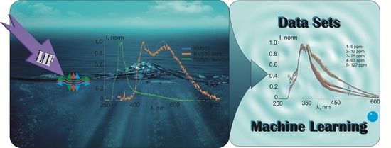
Firstly, the LIF spectra of the pure types of each oil product were measured to obtain etalons. There are distinctive distributions of the LIF spectra in Figure 3 for the different types of pure oil products which were discussed in the article, among which the heavy types of fuel are marked by dashed lines. The spectra were received by the radiation of the surface of the pure oil products volume in a back way (Figure 1). The left scale (Figure 3) is for the intensity of the light fuels including the DMZ, DMA, diesel fuel and the kerosene. The right one is for the heavier types of fuels such as RMB, RMG, RME and pure oil. The LIF spectral distributions were received in almost the same condition, and the values of the relative intensity (relative to the intensity at 295 nm) estimated the quantum efficiency of LIF for the different types of oil products. The values of the LIF intensities from the heavy types of fuels were smaller than the values from the light types, so we used 2 vertical axes to place these values in the linear scale. Subsequently, it was easy to note the distinctive differences of LIF spectra between the heavy and light types of fuel.
The long-pass filter Newport 10CGA-295 was used to reject the strong signal from the elastic scattering on the 278 nm wavelength. This filter rejected the radiation by 4 orders on the 278 nm of LED radiation wavelength. The full width at the half maximum (FWHM) of the LED radiation line was 15 nm. The small maximum was registered at the wavelength of 295 nm when the LED radiation crossed the filter with a nonuniform transmission of the spectral components.
LIF spectra of the crude oil and heavy types of marine fuel are presented by a homogeneous broad spectral line of 180–225 nm of the FWHM. The maximum of the spectral distribution is within the wavelength band from 480 to 540 nm, and it is a distinctive feature of the heavy types of fuel of the pure state. The other group of distinctive features unifies the pure light types of fuel. This group included a compound form of spectral distribution where maxima were shifted to the shorter range of wavelengths from 340 to 430 nm. This difference in the LIF spectra of the crude oil and the heavy types of oil from the light types of oil is well known [22,31,32]. Each type of light fuel in a pure state has its distinctive spectral distribution, which can be used for identification. Nonetheless, it is quite challenging to identify heavy fuels in a pure state by their types since the spectral distribution is almost the same.

3. Results of the Experimental Research

3.1. Spectral Features of LIF for a Different State of Oil Products

The change of LIF spectra was investigated when the fuel state changed from the pure to the slick state, and then to the solution. The forms of the spectral LIF distributions are shown as an example depending on the state of the oil product for the heavy RMB 30 fuel in Figure 4. The LIF spectrum of the pure seawater and background radiation was measured before the spectra of the slicks and solutions were measured. The signals from the seawater fluorescence and background radiation were excluded from the summarized LIF signal.
The LIF spectra of the RMB 30 pure fuel (blue), the RMB 30 slick with a thickness of 80 μm on the sea surface (orange) and of the RMB 30 solution with a concentration of 22.2 ppm (green) are shown in Figure 4. The line with the center of 295 nm had the same origin as the line in Figure 3. Normalized intensity is shown in the figure; it was normalized at the maximum value of the intensity in the spectral distribution of the LIF signal for each case. The values of the LIF intensity were very different. Such a method of normalization was used to compare the typical characteristics of LIF spectra of the different states, so the following specific change of the heavy fuel spectrum may be noticed. The shape of the spectra distribution changed when the pure fuel changed to the slick and then to the solution. Thus, this change is shown from the broad homogeneous line to the fairly narrow structured line. This fact shows the mechanism of interaction of fuel molecules with water molecules, i.e., this is the process of dissolution. This process was noticed when the structure of the slick spectrum was observed. An additional wide maximum appeared in the short wavelength from the center of the line. The features of the spectral changes of the light fuels were complicated, but still, they were changed in the same way. The spectrum of DMA, depending on its state, is shown in Figure 5.
The LIF spectrum of the solution is a narrower line compared to the spectrum of the pure fuel, and the center is placed on the short wavelength. The spectrum of the slick is an intermediate case. The additional maximum begins to form in the spectrum. This pattern was observed in almost all the investigated solutions of the light type fuels excluding kerosene. The shape of the spectral distribution was not changed much from a pure state to the solution in the case of kerosene. It is essential to mention that the form of the spectra of either the slicks or the solutions changed as time progressed (this fact for the solutions is described in Section 3.2, and the case of the slicks is described in [6,32]). The spectra of slicks (Figure 4 and Figure 5) were received right after the fuel was poured on to the seawater surface. The spectral distribution of the LIF depended on the state of the oil product in the seawater (i.e., solution or slick).

3.2. Features of the LIF Spectra of Oil Products in the Solution

The LIF method may be applied for the identification of oil product solutions, and it is necessary to have distinctive features of LIF for each of them. The investigation of the spectral distributions of the solutions was provided for each type of fuel and its different concentrations. The LIF spectra from the solutions of DMA and RMB 30 in different concentrations in the seawater are shown in Figure 6 and Figure 7, respectively. The values of the concentrations of the solutions are shown in ppm. They correspond to the particular color of the diagram and are placed in the upper right part of the figures.
The intensity of the spectral components was normalized at the intensity of the LED radiation (relative intensity is shown on the vertical scale). The spectra which are titled “seawater” correspond to the seawater with no solutions of oil products.
The differences in the fluorescence spectra of the DMA and RMB-30 solutions may be applied to recognize these types of fuels by the form of spectra using machine learning. Quite a narrow absorption line (at the wavelength of 346 nm) in the fluorescence spectrum is distinctive of the LIF spectra of the dissolved oil products in the seawater, unlike the slick or pure state. This absorption feature appeared in all the types of investigated solutions of the oil products and may be used to identify the dissolved fraction of oil pollution. The absorption feature in the fluorescence spectrum may also be used to measure the concentrations of oil products. Data sets for all the investigated types of dissolved oil products have been collected in the research. Five values of solution concentrations were prepared for all six types of fuel and crude oil. Data sets for each type of marine fuel included 30 LIF spectrums for each value of the concentration. Therefore, the total data set included 150 LIF spectra for each type of fuel. The shape of the LIF spectral distributions was used as a description for the identification of oil product type by machine learning. The program component was developed by machine learning to identify the solution of each oil product, which was investigated. Python with scikit-learn and NumPy libraries were used to carry it out. The spectra were preliminary processed, normalized and converted to a common format. Then, the array of the spectra of the different types of oil was used to collect the data set and receive features from it. The example of the LIF spectra data set, which was used for the machine learning of identification of the light type of fuel such as DMA is shown (Figure 8). The linear support vector classification (LinearSVC) algorithm was used to classify the spectra [33]. Five separate sequences of DMA fuel spectra are shown. Each sequence includes 30 spectra and corresponds to the exact concentration of oil products in the seawater. Values of the concentrations were 6 ppm (spectra # 1), 12 ppm (spectra # 2), 25 ppm (spectra # 3), 63 ppm (spectra # 4) and 127 ppm (spectra # 5), respectively.
The sequence of crude oil solutions within the range of concentration 0.6–13 ppm is shown in Figure 9. The data sets of these examples represent extreme cases in machine learning for the identification of different types of oil products (light fuel and crude oil) in dissolved states in the surface layer at sea.
It was planned to add the spectra of different concentrations for each type of vessel fuel to the data sets. It is necessary to mention that the magnitude order of the dissolved oil product concentrations may be received by way of spectral distribution. It could be additional information when the concentration was measured, and the oil product was recognized using machine learning. A value of integral spectral parameter α is offered to be measured for the concentrations detection of dissolved oil hydrocarbons and the calibration of LIF spectra with oil product concentrations; this value is as follows:
α = 300 525 ( I ( λ ) I 0 ( λ ) ) d λ ,
where I(λ)—the intensity of the total signal of LIF on the wavelength λ, I0(λ)—LIF signal of the seawater without dissolved oil products on the wavelength λ. The integration was done within 300–525 nm. Then, this parameter was calibrated with relevant concentrations of oil and oil products. The calibration function of the DMA solution is shown in Figure 10 as an example of the calibration of the LIF method. The LoD value of this oil product in the seawater may be received by this function. A regression estimation of experimental data was used, and the values of the minimum detectable concentrations were estimated by the criteria of LoD = 3n/S, where n—standard deviation of LIF signal, S—calibration line slope [34].
The values of the integral parameter of the spectral distribution—α for the DMA solutions of different concentrations are at the vertical scale (Figure 10). DMA spectra of relative concentrations are shown in Figure 6. The values of the concentrations were calibrated by the standard method of Fourier transform infrared spectroscopy. Such calibration was done for all the investigated types of light and heavy fuels and, crude oil. The LoD values of the oil products in the solution of the investigated fuel were measured using these calibrations. The LoD values are reported in Table 1.
LoD values are to apply the LIF for bilge water disposal monitoring and control. Nonetheless, LoD values strongly depend on the daylight background. Moreover, they depend on how the sensor is used (LIDAR or submersible sensor). In this research, 278 nm of wavelength was used, so it was possible to measure LIF within the wavelength band with minimal daylight background. The LIF spectrum was received with a daylight background (Figure 11). This spectrum was received by the LIF sensor at 1 m of height above the surface of the solution (the setup is in Figure 1).
The measurements were obtained on a sunny day at 2 p.m. (local time). The intensity of the solar background at the laboratory was comparable to the outdoor solar background. The measurement was obtained for four concentrations of DMA solutions in the seawater (42, 21, 14 and 2 ppm), and it was possible to value the LoD. It was 18 ppm for the DMA. The wavelength band of 320–430 nm of the spectrum was used to measure the α coefficient at the daylight background. The LIF signals were received in this band and higher than the background radiation which included the sunlight and the LIF of the seawater surface (seawater + sun on Figure 11) with no DMA solution. The background signal was higher than the LIF signal in the more longwave band. It is caused by the strong absorption of radiation by the solution and the weak signal of LIF from the DMA solution within this band. The measurement of the background (LIF from water and daylight) was done before the solution was added to the seawater. Nonetheless, oil products in the slick or solution become degraded at sea [31], and their LIF spectra are changed [24]. The degradation is caused by an environmental condition that influences the molecule complexes of oil products and their fluorescence features are changed. The dynamics of the fluorescence spectra of the aforementioned solutions of fuel types were investigated. There is an example of a change of the LIF spectral distribution for DMA in Figure 12.
Different colors correspond to the different concentrations of solutions in Figure 12. The spectral distributions of solutions after five days of dissolution are marked by the dashed lines. The intensity of the signal was reduced more than twice for all the measured concentrations after five days. Almost the same change of the fluorescence intensity was being observed for the other types of fuels. Nonetheless, some change in the spectral distribution form can be noticed and used as distinctive features for the age of solution recognition.

3.3. Features of LIF Spectral Distribution from Slick

The measurement of the LIF spectra from the oil product slicks was well researched and described in scientific articles. Nonetheless, in this research, the experiments were conducted to investigate the limits of recognition for some types of slicks of the exact types of fuels by the shape of spectra using machine learning. This investigation was aimed to establish the following questions:
-
Is the shape of the LIF spectra from researched types significantly different?
-
How does the thickness of the same types of slicks influence the shape of the LIF spectra?
-
How long do these differences last as the slick is degrading?
The laboratory research of the LIF spectra from the slicks was obtained for several types of light and one heavy marine fuel. It is necessary to mention that it is quite hard to measure the slicks, especially those of heavy types. The thickness of the slick is not homogenous. Even at the laboratory, it was not possible to obtain a homogenous thickness of the slick, especially those of heavy types of fuel just after the slick was prepared. There were areas of high and low values of slick surface thickness. The following values of the slick thickness are the average of the minimum and maximum thicknesses which were observed on the slick. Thus, the research on the distinctive features of the LIF spectral distribution for different values of thickness was conducted for the light types of marine fuels only. Concerning the heavy types of marine fuels, the measurements were obtained for the RMB slick only with a thickness of 80 µm (Figure 4). Features of the LIF spectral distribution of slicks of different types and thickness were analyzed using the experimental data of the slick spectra of the light types of fuels. Slick spectra of 20, 100, 300 and 500 µm thickness were measured, and the example of such distribution is shown in Figure 13. Different colors in the upper part correspond to the different types of slicks.
Distinctive types of spectral distributions for each type of investigated fuel slicks were observed. It is possible to develop program methods for the identification of the fuel types as slicks by LIF spectra using machine learning. Nowadays, the data sets of the LIF spectra of slicks from light types of vessel fuels are being collected in the same way as it had been done for light types of vessel fuel solutions. The spectra of the DMA from the slicks of different thicknesses are shown in Figure 14, and each thickness of the slick corresponds to different colors in the upper part of the picture. The spectral distribution of the LIF slick from 20 µm to 500 µm almost coincides.
The results of the dynamics research on LIF spectra from slicks show that the form of the spectra were not significantly changed in our case where the process of dissolution of the slick was the main process in weathering.

4. Discussion

Experimental results showed that the shapes of LIF spectra changed significantly depending on the state of the oil product. The spectral distribution of the LIF for the same oil products was quite different and depended on the state (pure state, slick or solution). The dissolved fraction caused a fairly narrow maximum in the spectra of the oil products and this maximum was displaced to the shortwave band. The spectra of the oil product slicks are the intermediate stage of the spectrum between the pure fuel and the solution. This phenomenon should be concerned when the LIF method was used to identify the types of oil products in the bilge water or the slick on the sea surface. It is necessary to have etalons of the LIF spectra of oil products in the relevant state in which it can be found in the oil pollution (slick or solution state). The shape of the solution lines has the maximum within the band of 330–370 nm, and the full width at half maximum is about 40–70 nm. The spectra with a distinctive shape of each type may be used as specific characteristics for the recognition by machine learning. Heavy types of fuel have typical tails of the spectral distribution within the wavelength band of 400–550 nm. Narrow lines of absorption were observed in the LIF spectrum within a 320–360 nm band. There could be several absorption lines for the heavy types. The absorption feature of the LIF of the solutions of the researched oil products at the 346 nm was distinctive. This therefore indicates that if there is a dissolved fraction of oil product, it may be used to measure concentrations of oil products in the solution as well as the integral α parameter of the fluorescence spectra. It may be useful if there are different types of oil products in the bilge water.
The LIF method provided low values of LoD by the integral α parameter of the LIF spectra. The calibration is a linear function with quite a wide range of concentration values. LoD values are much lower than the threshold limit values which were established for the bilge water by MARPOL. Nonetheless, such LoD values were received with almost no solar radiation, and the setup of the submersible sensor was used in the time of measurements. LoD values rise high when the measurement was provided in daylight or by sensor used as a LIDAR (sensing through seawater surface).
In the case of light types of marine fuel, the shortwave radiation of LIF contributes significantly to the integral parameter α, while the sunlight emission contributes much more in the case of crude oil and heavy types of fuel. The LIF spectra from dissolved oil hydrocarbons were possible to register at daylight since UV radiation with 278 nm of wavelength was used. The laser radiation of 355 nm and 412 nm of wavelength were used by [24,25], but the authors received LIF spectra of oil product slicks on the water surface with no daylight.
The comparison of the LoD values with no solar emission in the submersible spectrometer regime with the LIDAR regime in daylight was made. The LoD values of the crude oil solution raised to 23 ppm (0.12 ppm in the night), DMA solution to 18 ppm (0.1 ppm in the night), DMZ solution to 17 ppm (1.1 ppm in the night) and the RMG 380 to 20 ppm (0.1 ppm in the night) with a solar emission background.
It is essential to provide additional research in situ to find out the exact limits to control bilge water promptly. The LoD for the LIDAR way of using may be reduced by increased integration time. Nonetheless, it could be used even in this way to control promptly if the concentrations of the oil products in the bilge water were limited. The submersible way might be used to measure smaller values of concentrations of dissolved oil products.
Experiments showed that the shape of the LIF spectra from solutions and fluorescence intensity changed as time passed. It may be caused by the diverse weathering processes of oil hydrocarbons. It is not easy to simulate natural weathering conditions of the sea at the laboratory. The samples were prepared and investigated, so that the influence of the dissolution on the complexes would be leading the process. This makes the shape of the LIF spectrum change or it reduces the quantum efficiency of the fluorescence since the research was aimed to improve the LIF for the recognition of oil product solutions.
Dynamic research of the LIF spectra from the solutions shows that the shape of the LIF spectra was not significantly changed if the weathering was minimized. Nonetheless, the efficiency of LIF reduces significantly (more than two times in five days). More significant changes in the LIF efficiency were caused by photochemical weathering and vaporization [31]. The appearance of the spectral component in the shortwave range from the main maximum and the reduction of the fluorescence signal was observed. It should be concerned when the concentration of oil products were measured. In addition, such dynamics of the LIF spectra should be of concern when methods of machine learning for fuel type identification by LIF spectra are being developed. It is essential to develop a dynamic matrix of features for each type of fuel. The procedure of machine learning should include either the identification of fuel type or the time when the oil product enters the seawater.
The spectra of the LIF slicks from the oil products were researched in many works. In this research, the investigation of the LIF spectra was aimed to be used for machine learning (data sets collection of the researched types of fuel) and to define the distinctive features of the LIF spectra in the time of excitation by UV radiation. The spectral features of LIF from the slicks of light fuels only were studied. The band of the slick thickness from 20 µm to 500 µm was studied. The main results obtained agreed with the results in [6,17,24,25]:
-
The LIF spectra almost agreed for the different thicknesses of the slicks of the same type of fuel. For now, it is not possible to receive information about the slick thickness from LIF spectra. It is crucial to find new solutions for LIF application to receive this information;
-
The study of slick dynamics from the light type of fuels showed that the spectral distribution form of the LIF spectra of thin slick (20–300 µm) does not change much.
The study of the LIF spectra from the slicks of heavy types of fuel was complicated, and it was not managed to receive great statistics of measurements for different thicknesses. It was caused by a robust heterogeneous thickness of the slick surface. As a result, the LIF spectra were a sum of all the spectral distributions from different thicknesses. Thus, the spectral features of some slicks and thicknesses were being smoothed. This factor will be more crucial at sea because there will be many environmental influences on the slick and it will cause the rise of the slick thickness range. It is essential to provide additional in situ measurements.
The results of the light types of fuels may be already used in machine learning for the oil product identification of slicks by the LIF. The spectral distribution of LIF features is specific for the investigated types of oil products. Concerning heavy types of marine fuel, additional in situ research is essential to investigate how thickness and its distribution in the slick are spread under the environmental influence. It is crucial to provide numerous measurements and collect data sets of LIF spectra features for machine learning to identify heavy types of fuel. Today, the quantity of such data sets is lacking. The small-sized LIF sensor is being tested for UAV to collect a comparative data set in situ. The advantages of using UV radiation are as follows: the ability to monitor slicks and dissolved oil hydrocarbons at daylight; the high values of the quantum efficiency of LIF if UV radiation is used.
The disadvantages are as follows: heights are low due to the absorption of the atmosphere and LIF spectra are obtained from the very surface of the seawater (due to the strong absorption in the seawater); this is not crucial for the slicks, but this could be important for the solutions.
The values of the solution concentration in the upper layer of the ocean and under the surface may vary quite significantly. It is essential to provide measurement in the on-land regime and under the surface.

5. Conclusions

The LIF spectra dependence on oil product type and state is complicated. The form of LIF spectral distribution changes as time progresses. Nonetheless, still the research of these dependencies allows using this method to identify features of different types of marine fuel which are dissolved in the seawater or are promptly in the slick.
The identification and measurement of dissolved oil products in the seawater are the strong potential of using this method. This method can be well used to control such a giant source of ocean pollution as bilge water disposal by vessels, especially concerning the low values of LoD.
Monitoring methods that are based on the LIF spectroscopy may be used to identify the oil products that built up the slick. It is necessary to provide further research so that it will be possible to determine the dependence of LIF spectra parameters on slick thickness. It is quite perspective to use UAV for either regional-scale monitoring or collecting LIF spectra data sets. It will be used to provide machine learning for the identification of oil product type and the measurement of pollution volume as a solution state and slick.

Author Contributions

O.B.—conceptualization and methodology; D.P.—investigation, C.A.—software; D.K.—investigation; I.B.—investigation; V.Y.—writing and project administration; I.S.—validation, A.N.—validation. All authors have read and agreed to the published version of the manuscript.

Funding

This research was funded by the Federal Agency for Maritime and River Transport (applied research and technical development) and Grant # 19-72-00107 by the Russian Science Foundation (the fundamental research of the LIF spectra formation and Artificial Intelligence development).

Acknowledgments

This research was supported by the Federal Agency for Maritime and River Transport (applied research and technical development) and Grant # 19-72-00107 by the Russian Science Foundation (the fundamental research of the LIF spectra formation and Artificial Intelligence development).

Conflicts of Interest

The authors declare no conflict of interest.

References

  1. Kinsey, J.L. Laser-induced fluorescence. Annu. Rev. Phys. Chem. 1977, 28, 349–372. [Google Scholar] [CrossRef]
  2. Gabbarini, V.; Rossi, R.; Ciparisse, J.-F.; Malizia, A.; Divizia, A.; De Filippis, P.; Anselmi, M.; Carestia, M.; Palombi, L.; Divizia, M.; et al. Laser-induced fluorescence (LIF) as a smart method for fast environmental virological analyses: Validation on Picornaviruses. Sci. Rep. 2019, 9, 12598. [Google Scholar] [CrossRef] [PubMed] [Green Version]
  3. Demtroder, W. Laser Spectroscopy; Springer: Berlin/Heidelberg, Germany; New York, NY, USA, 1996; pp. 414–424. [Google Scholar]
  4. Raymond, M. Laser Remote Sensing: Fundamentals and Application; Krieger Publishing Company: Malabar, FL, USA, 1984; pp. 127–282. [Google Scholar]
  5. Frank, U. A review of fluorescence spectroscopic methods for oil spill source identification. Toxicol. Environ. Chem. Rev. 1978, 2, 163–185. [Google Scholar] [CrossRef]
  6. Utkin, A.B.; Lavrov, A.; Vilar, R. Evaluation of oil spills by laser induced fluorescence spectra. In International Conference on Lasers, Applications, and Technologies, Kazan, Russian Federation, 23–27 August 2010; Vladislav, P., Gérard, M., Aleksei, M.Z., Eds.; International Society for Optics and Photonics: Bellingham, WA, USA, 2011; Volume 7994, p. 799415. [Google Scholar]
  7. Chen, P.; Li, Y.; Liu, B.; Xu, J. Oil spill information exaction by laser fluorescence. In Proceedings of the 2014 IEEE Geoscience and Remote Sensing Symposium, Québec, QC, Canada, 13–18 July 2014; pp. 4355–4357. [Google Scholar]
  8. Fingas, M.; Brown, C.E. A review of oil spill remote sensing. Sensors 2018, 18, 91. [Google Scholar] [CrossRef] [Green Version]
  9. Fingas, M. The Challenges of Remotely Measuring Oil Slick Thickness. Remote Sens. 2018, 10, 319. [Google Scholar] [CrossRef] [Green Version]
  10. Jha, M.N.; Levy, J.; Gao, Y. Advances in Remote Sensing for Oil Spill Disaster Management: State-of-the-Art Sensors Technology for Oil Spill Surveillance. Sensors 2008, 8, 236–255. [Google Scholar] [CrossRef] [Green Version]
  11. Brown, C.; Fingas, M. Review of the development of laser fluorosensors for oil spill application. Mar. Pollut. Bull. 2003, 47, 477–484. [Google Scholar] [CrossRef]
  12. Chirita, A.; Kukhtarev, N.; Dimov, F. Detection of thin oil films on water surface from a remote distance when fluorescence is excited by 447nm laser light. J. Optoelectron. Adv. Mater. 2017, 19, 184–188. [Google Scholar]
  13. Bukin, O.A.; Proschenko, D.; Chekhlenok, A.; Golik, S.S.; Bukin, I.; Mayor, A.Y.; Yurchik, V. Laser Spectroscopic Sensors for the Development of Anthropomorphic Robot Sensitivity. Sensors 2018, 18, 1680. [Google Scholar] [CrossRef] [Green Version]
  14. Babichenko, S.; Beynon, D.; O’Neill, K. Submerged-oil tracking by airborne hyperspectral fluorescent lidar. SPIE Newsroom 2010, 10, 003273. [Google Scholar] [CrossRef]
  15. Robbe, N.; Hengstermann, T. Remote Sensing of Marine Oil Spills from Airborne Platforms Using Multi-Sensor Systems. WIT Trans. Ecol. Environ. 2006, 95, 347–355. [Google Scholar]
  16. Hoge, F.E.; Swift, R.N. Oil film thickness measurement using airborne laser-induced water Raman backscatter. Appl. Opt. 1980, 19, 3269–3281. [Google Scholar] [CrossRef] [PubMed]
  17. Babichenko, S.; Poryvkina, L.; Rebane, O.; Sobolev, I. Compact HLIF LiDAR for marine applications. Int. J. Remote Sens. 2016, 37, 3924–3937. [Google Scholar] [CrossRef] [Green Version]
  18. Utkin, A.; Lavrov, A.; Vilar, R.; Cruz, I. Optical Methods for Water Pollution Monitoring. In Spatial and Organizational Dynamics Discussion Papers; CIEO-Research Centre for Spatial and Organizational Dynamics, University of Algarve: Noronha, Brazil, 2011; Volume 17, pp. 129–146. [Google Scholar]
  19. Vasilescu, J.; Marmureanu, L.; Carstea, E.; Cristescu, C.P. Oil spills detection from fluorescence lidar measurements. Univ. Politeh. Buchar. Sci. Bull. Ser. A Appl. Math. Phys. 2010, 72, 149–154. [Google Scholar]
  20. Leifer, I.; Lehr, W.J.; Simecek-Beatty, D.; Bradley, E.; Clark, R.; Dennison, P.E.; Hu, Y.; Matheson, S.; Jones, C.E.; Holt, B.; et al. State of the art satellite and airborne marine oil spill remote sensing: Application to the BP Deepwater Horizon oil spill. Remote Sens. Environ. 2012, 124, 185–209. [Google Scholar] [CrossRef] [Green Version]
  21. Babichenko, S. Laser remote sensing of the European marine environment: LIF technology and applications. In Remote Sensing of the European Seas; Springer: Dordrecht, The Netherlands, 2008; pp. 189–204. [Google Scholar]
  22. MacHutchon, K.R. Airborne laser induced fluorescence as a means for the effective management of oil spills, and for the enforcement of oil discharge regulations. Trans. Built Environ. 2003, 70, 185–194. [Google Scholar]
  23. Bollmann, M. World Ocean Review: Living with the Oceans; Maribus: Hamburg, Germany, 2010; pp. 92–99. [Google Scholar]
  24. Raimondi, V.; Palombi, L.; Lognoli, D.; Masini, A.; Simeone, E. Experimental tests and radiometric calculations for the feasibility of fluorescence LIDAR-based discrimination of oil spills from UAV. Int. J. Appl. Earth Obs. Geoinf. 2017, 61, 46–54. [Google Scholar] [CrossRef]
  25. Duan, Z.; Li, Y.; Wang, J.; Zhao, G.; Svanberg, S. Aquatic environment monitoring using a drone-based fluorosensor. Appl. Phys. 2019, 125, 108. [Google Scholar] [CrossRef] [Green Version]
  26. Julian, M. MARPOL 73/78: The International Convention for the Prevention of Pollution from Ships. Marit. Stud. 2000, 2000, 16–23. [Google Scholar] [CrossRef]
  27. Puiu, A.; Fiorani, L.; Menicucci, I.; Pistilli, M.; Lai, A. Submersible spectrofluorometer for real-time sensing of water quality. Sensors 2015, 15, 14415–14434. [Google Scholar] [CrossRef] [Green Version]
  28. Deqing, L.; Xiaoning, L.; Jinjia, G.; Tingwei, C.; Jubai, A.; Ronger, Z. A New Approach of Oil Spill Detection Using Time-Resolved LIF Combined with Parallel Factors Analysis for Laser Remote Sensing. Sensors 2016, 16, 1347. [Google Scholar]
  29. EN 590: 2009 + F1:2010 Automotive Fuels-Diesel-Requirements and Test Methods. Available online: https://infostore.saiglobal.com/preview/98696798931.pdf?sku=883793_SAIG_NSAI_NSAI_2099445 (accessed on 26 February 2020).
  30. ISO 8217: 2012 Petroleum Products-Fuels (Class F)-Specifications of Marine Fuels. Available online: https://www.iso.org/standard/59479.html (accessed on 26 February 2020).
  31. Nicodem, D.E.; Guedes, C.L.B.; Correa, R.J. Photochemistry of petroleum: I. Systematic study of a brazilian intermediate crude oil. Mar. Chem. 1998, 63, 93–104. [Google Scholar] [CrossRef]
  32. Fedotov, Y.V.; Belov, M.L.; Kravtsov, D.A.; Gorodnichev, V.A.; Stepanov, R.O. Comparative laser-induced fluorescence evolution analysis of different oil pollution on the terrestrial surface. IOP Conf. Ser. Mater. Sci. Eng. 2019, 537, 022019. [Google Scholar] [CrossRef]
  33. Cortes, C.; Vapnik, V. Support-vector networks. Mach. Learn. 1995, 20, 273–297. [Google Scholar] [CrossRef]
  34. Cremers, D.A.; Radziemski, L.J. Handbook of Laser-Induced Breakdown Spectroscopy; JohnWiley & Sons, Ltd.: New York, NY, USA, 2006. [Google Scholar]
Figure 1. Smallsized laser-induced fluorescence (LIF) spectrometer. 1—Maya 2000Pro spectrometer, 2—laser diode 6060 UVS LED; 3—collimator (quartz lens); 4—radiator for LED; 5—collimator (lens 84-UV, this channel for LIDAR sounding); 6—84-UV-25 collimator (Ocean Optics); 7—fiber-optic light guide P600-2-SR (Ocean Optics, this channel is open in the on-land regime, but closed in the LIDAR sounding); 8—computer ITX-N29; 9—quartz port-light; 10—holding of MAYA 2000Pro and computer; 11—holding of lens.
Photonics 07 00036 g001
Figure 2. The laboratory set-up for the investigation of the LIF spectra of oil product solutions. 1—radiator with LED; 2—quartz lens; 3—solution of oil product in the cuvette; 4—filter (Newport 10CGA-295); 5—spectrometer Maya 2000Pro; 6—74-UD collimator (Ocean Optics); 7—quartz optical windows.
Photonics 07 00036 g002
Figure 3. Oil product LIF spectra of the pure state.
Photonics 07 00036 g003
Figure 4. LIF spectra of the heavy RMB 30 marine fuel depending on its state.
Photonics 07 00036 g004
Figure 5. LIF spectra of the light DMA fuel depending on its state.
Photonics 07 00036 g005
Figure 6. LIF spectra of the DMA solutions.
Photonics 07 00036 g006
Figure 7. LIF spectra of the RMB 30 solutions.
Photonics 07 00036 g007
Figure 8. Sequences of the LIF spectra of the five concentrations of DMA solutions.
Photonics 07 00036 g008
Figure 9. Sequences of the LIF spectra of the five concentrations of crude oil solutions.
Photonics 07 00036 g009
Figure 10. The calibration function for the DMA solution by α as the integral parameter.
Photonics 07 00036 g010
Figure 11. LIF spectrum of the DMA with a daylight background by LIDAR sounding.
Photonics 07 00036 g011
Figure 12. Dynamics of the DMA spectra for 5 days.
Photonics 07 00036 g012
Figure 13. LIF slick spectra of the different types of oil products.
Photonics 07 00036 g013
Figure 14. The form of the LIF spectra from the DMA slicks of different thicknesses.
Photonics 07 00036 g014
Table 1. Limit of detection (LoD) values for the various oil products.
#Type of Oil ProductsLoD (ppm)
1DMA0.1
2DMZ1.1
3RMB 300.3
4RME 1800.2
5RMG 3800.1
6Diesel oil0.7
7Crude oil0.1
8Kerosene2.4

