Flowline Optical Simulation to Refractive/Reflective 3D Systems: Optical Path Length Correction

Abstract

Nonimaging optics is focused on the study of techniques to design optical systems for the purpose of energy transfer instead of image forming. The flowline optical design method, based on the definition of the geometrical flux vector J, is one of these techniques. The main advantage of the flowline method is its capability to visualize and estimate how radiant energy is transferred by the optical systems using the concepts of vector field theory, such as field line or flux tube, which overcomes traditional raytrace methods. The main objective this paper is to extend the flowline method to analyze and design real 3D concentration and illumination systems by the development of new simulation techniques. In this paper, analyzed real 3D refractive and reflective systems using the flowline vector potential method. A new constant term of optical path length is introduced, similar and comparable to the gauge invariant, which produces a correction to enable the agreement between raytrace- and flowline-based computations. This new optical simulation methodology provides traditional raytrace results, such as irradiance maps, but opens new perspectives to obtaining higher precision with lower computation time. It can also provide new information for the vector field maps of 3D refractive/reflective systems.

1. Introduction

The concept of flowline and its associated geometrical flux vector, J, was first introduced as a photometrical theory by Gershun [1] and later developed by Moon [2]. Such a concept applies vector field theory to the study of irradiance transfer, which is based on the definition of the geometrical flux vector J produced by a Lambertian source at any point in the space P. The modulus of J is the maximum irradiance value at point P; the direction of the vector is the direction of the maximum irradiance at P. The projection of the J vector upon a plane directly corresponds to the irradiance on that plane. Over the last decades, vector flowline formalism has been applied to several problems in optics. In the seventh decade of last century, Winthrop [3] applied it to the study of propagation of structural information; at the end of that decade, Winston [4,5] applied it successfully to the study of concentrators, showing that reflective concentrators with the geometry of the field lines achieve the theoretical limit of concentration. Later, Welford and Winston [6] developed this method among others to create a new topic called nonimaging optics. Recently, flowline method has been used to design so-called hyperparabolic concentrators (HPC) [7], which extends the compound parabolic concentrator (CPC) to multiple reflections and approaches the thermodynamic limit of concentration. Another interesting result from the application of field theory concepts to optical design is that refractive elements with the geometry of orthogonal surfaces to the field lines produce ideal concentrators [8].

This theoretical approach to the vector field theory of irradiance nowadays is focused on what can be described as “academic results”. In the other words, existing literature focuses on the design of optical systems with ideal light sources, ideal optical properties (reflectance and transmittance), and simple analytical optical geometries (parabolic, elliptic, and so on). It is clear that the capabilities of this powerful tool for real optical systems design have not yet been fully developed. The main objective of the present paper is the application of the flowline method and its related vector field theory to the analysis of real nonimaging 3D optical systems. In the previous paper [9], we successfully applied flowline method to the analysis of 2D optical systems, including reflective and refractive systems. In this paper, we address the complex problem of real 3D systems. In Section 2, we first establish theoretical vector potential background and apply it to free space light propagation; in Section 3, we apply the theoretical background to simple 3D source lens detector system; in Section 4, we apply the theoretical background to simple 3D source reflector detector system; in Section 5, from the analysis of the obtained results, we introduce a constant term in the optical path length (OPL) in a similar way to gauge invariant, which corrects the theoretical model and provides a good agreement between flowline and raytrace simulation results; and finally, in Section 6, the conclusion is given.

2. Theoretical Background and Flowline Methodology for 3D Optical Systems Analysis

As we have mentioned previously, the flowline method was developed by Winston and Welford [4,5,6] was based on the concept of geometrical flux vector J, in the context of applying the etendue conservation law for a loss-free optical system. The Cartesian components of the geometrical flux vector J are

$$J_x={\displaystyle \int }d{p}_{y}d{p}_z,J_y={\displaystyle \int }d{p}_{x}d{p}_z,J_z={\displaystyle \int }d{p}_{x}d{p}_y$$

(1)

where dp_x, dp_y, and dp_z are the direction cosines or, for more general considerations, the generalized optical momenta in phase space. The physical meaning of geometrical flux vector is that the J_z component at any point in the space P, for instance, is proportional to the total flux per unit area (irradiance/illuminance) entering to a plane parallel to the XY plane at point P. The most important property of flowline method is that it represents a new way to construct concentrators with maximum concentration ratio, which is to place mirrors with the geometry of flowlines [6]. In an analogous way, following Gershun [1], the concept of light vector was introduced, and the magnitude of light vector equals the net radiant power per unit area at point P, and the direction of the vector is the direction of the flow of the radiant energy at that point. To analyze 3D optical systems, we used the concept of vector potential of this light vector, in way that the geometrical flux vector can be computed from vector potential A [1] as

$$\mathbf{J}=\mathrm{curl}\mathbf{A}$$

(2)

where

$$\mathbf{A}=\frac{B}{2}{\displaystyle \oint }\ln r\mathit{d}\mathit{l}$$

(3)

where r is the distance between the contour of the source and any point P in the space. The integral is calculated for the closed contour of the light source, and dl is an infinitesimal vector along the direction of the contour of the light source. B is the luminance/radiance of the source—it is a constant for Lambertian radiators and therefore we can get it out of the integral.

The methodology followed in the present paper is to compute the J vector indirectly from vector potential computation for different real 3D optical systems. We will replace r by the optical path length, L, in Equation (3) for systems with refractive elements. One of the potential advantages of the proposed flowline method is the computation of a contour integral, Equation (3), instead of the surface computation needed for raytrace, as it can improve computation efficiency. Another potential advantage of the flowline method is the possibility of calculating field lines, which provides information about the energy flow related with ideal optical designs. We studied optical systems with an optical axis coincident to the OZ axis, and we analyzed irradiance distribution at a detector plane perpendicular to the optical axis, and then we computed the J_z component at the detector plane. We also compared the results obtained from the computation of Equations (2) and (3) of J_z with raytrace computations.

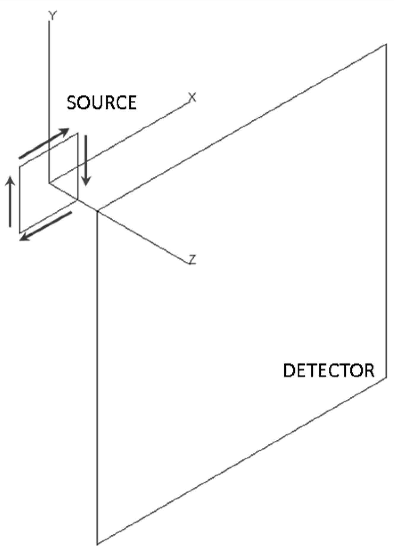
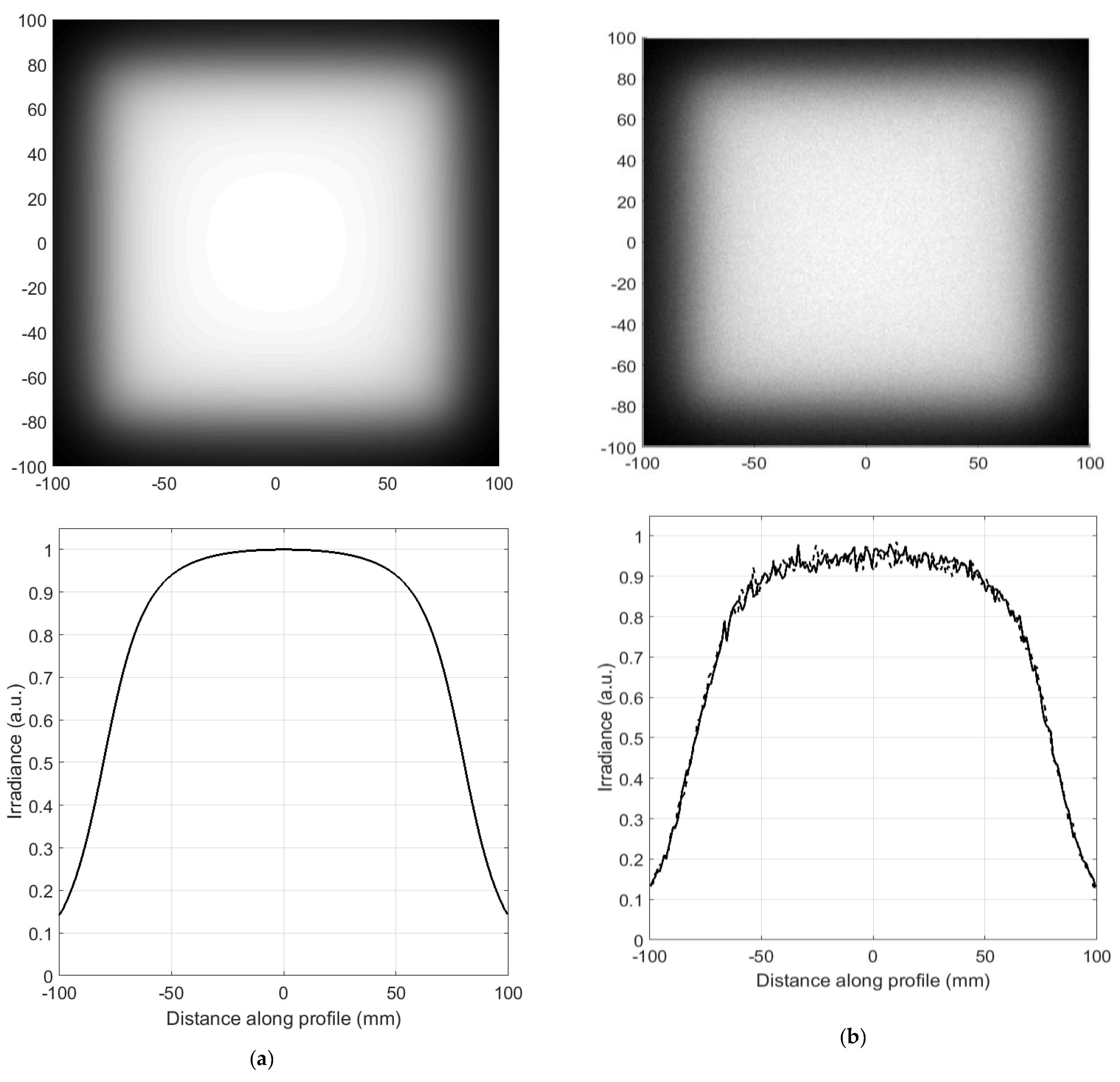
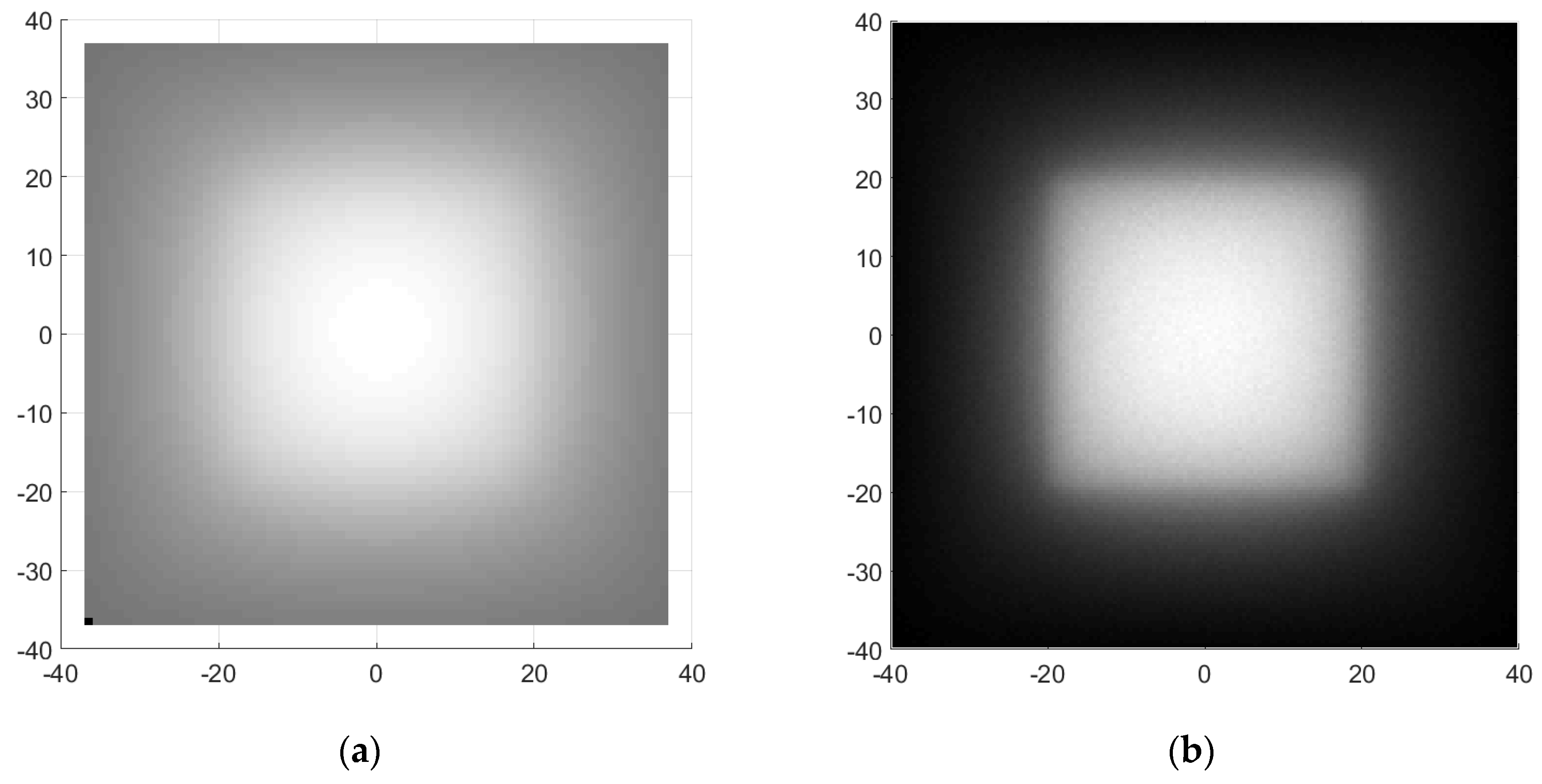
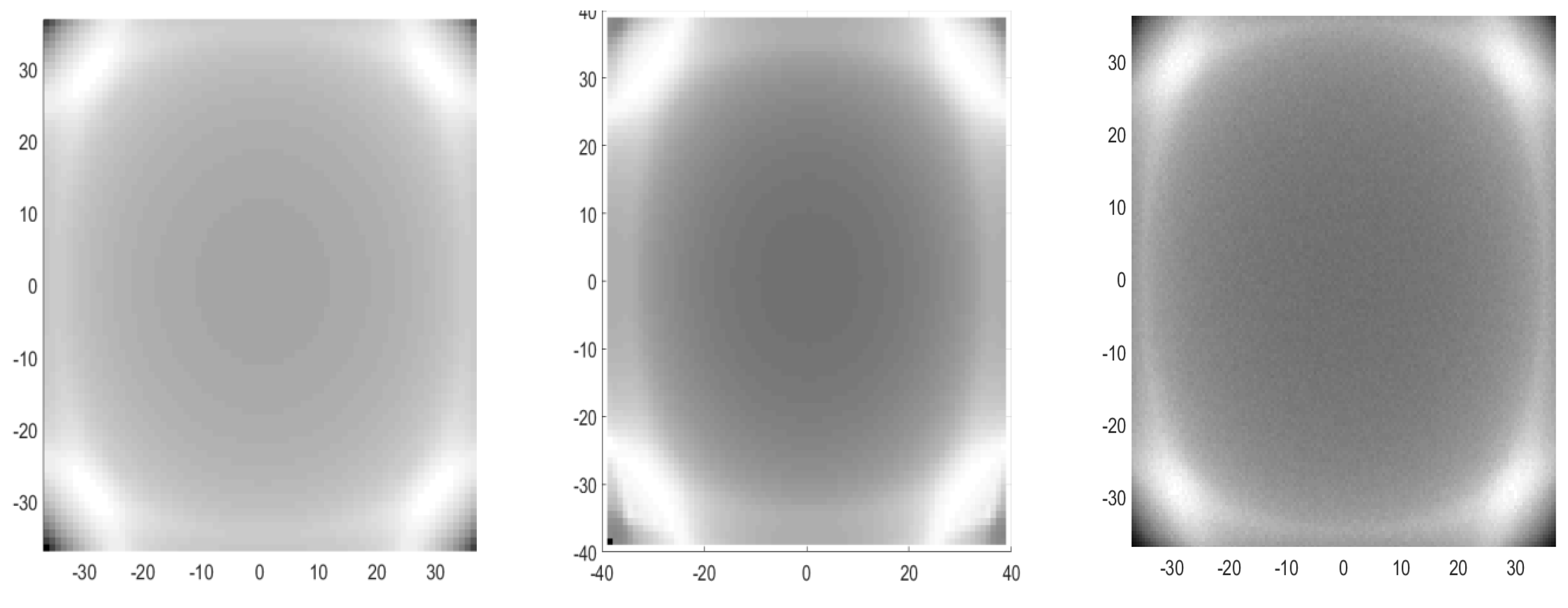
Irradiance Computation from J Vector for Simple Free Space 3D Non Symmetric Systems

To advance the objective of establishing the methodology for optical simulation based on flowline computation, we studied some simple examples of asymmetric optical systems. We started with square and rectangular sources. The sources lay in the XY plane, and with OZ as the optical axis, we computed an irradiance map orthogonal to the optical axis for different configurations of sources and detectors. Figure 1 shows the sketch for the optical configuration to be analyzed. The irradiance E at detector can be computed as

$$E=J_z=\left(\frac{\partial A_y}{\partial x}-\frac{\partial A_x}{\partial y}\right).$$

(4)

Figure 2, Figure 3 and Figure 4 show the irradiance maps, and Figure 2a, Figure 3a and Figure 4a demonstrate flowline computation of irradiance on the basis of Equations (2) and (3) using Matlab software for different square and rectangular Lambertian sources. Figure 2b, Figure 3b and Figure 4b demonstrate the corresponding irradiance map computed by raytrace software [10]. The results show a clear agreement between the two methodologies of optical computation.

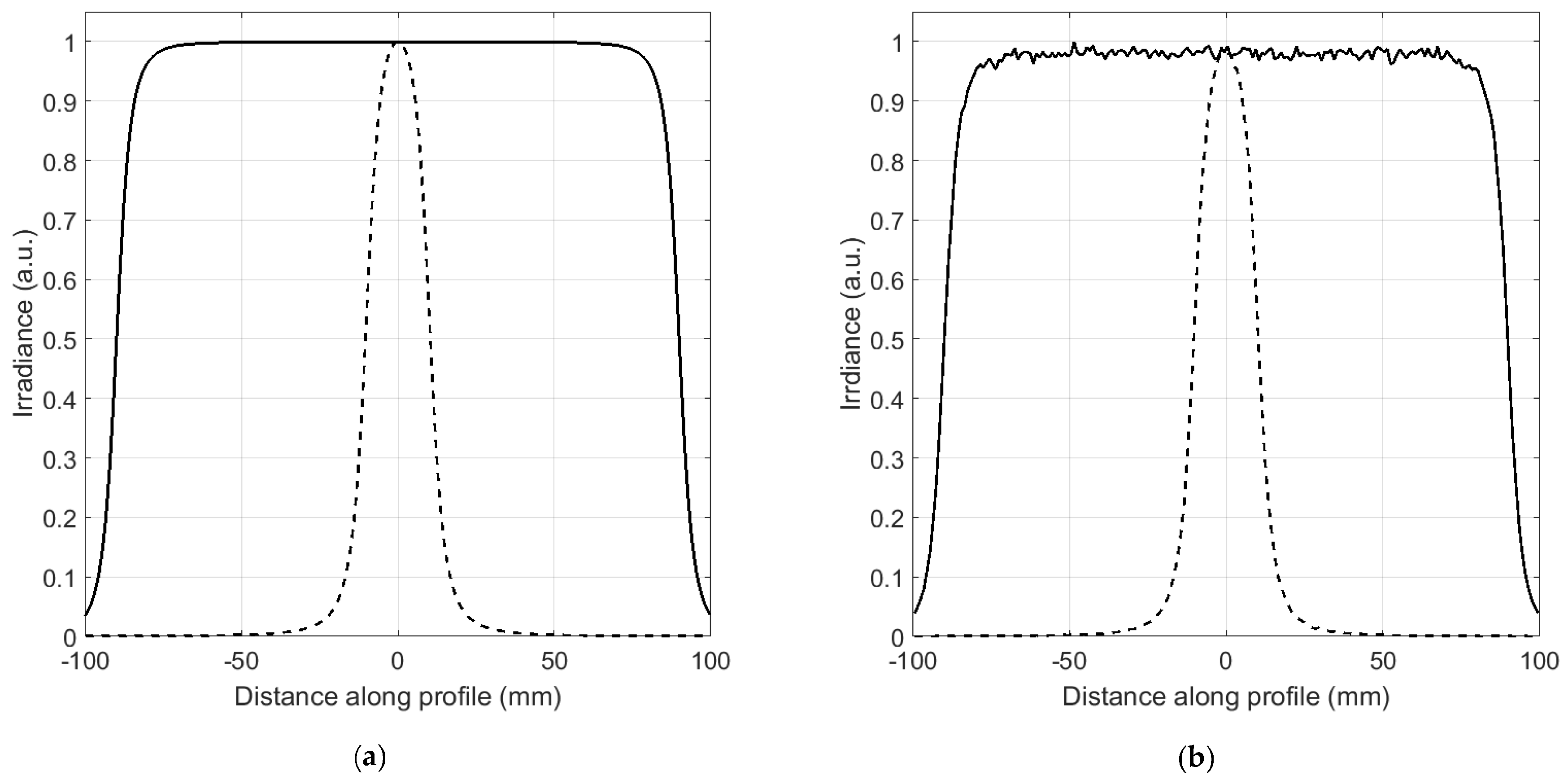
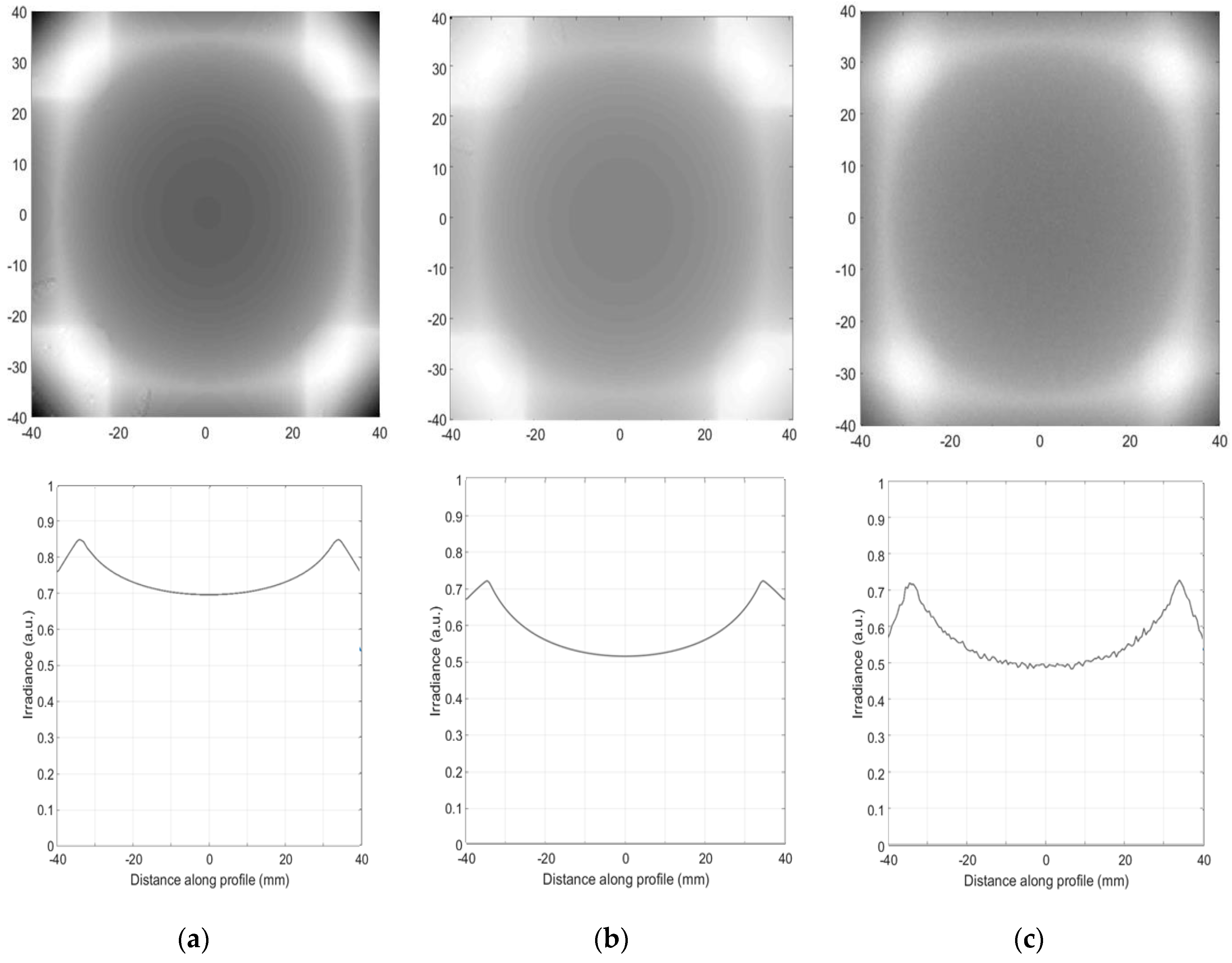
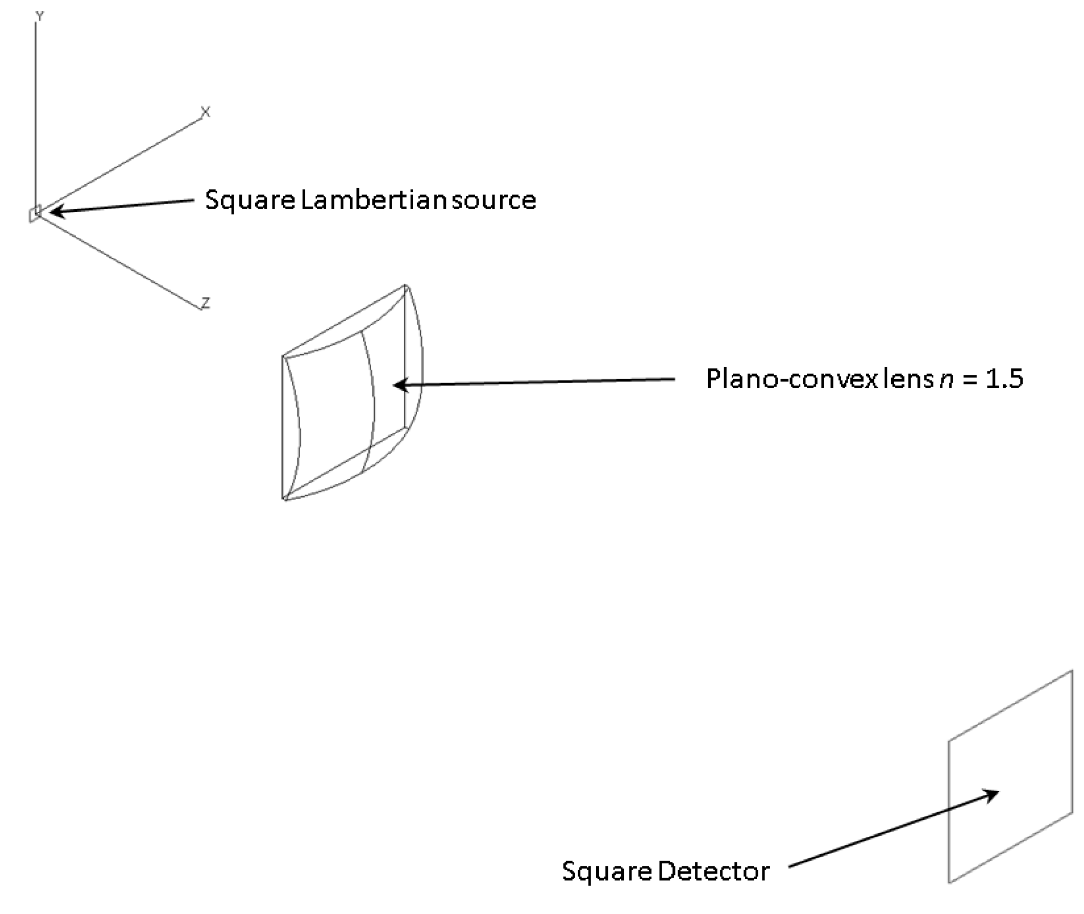
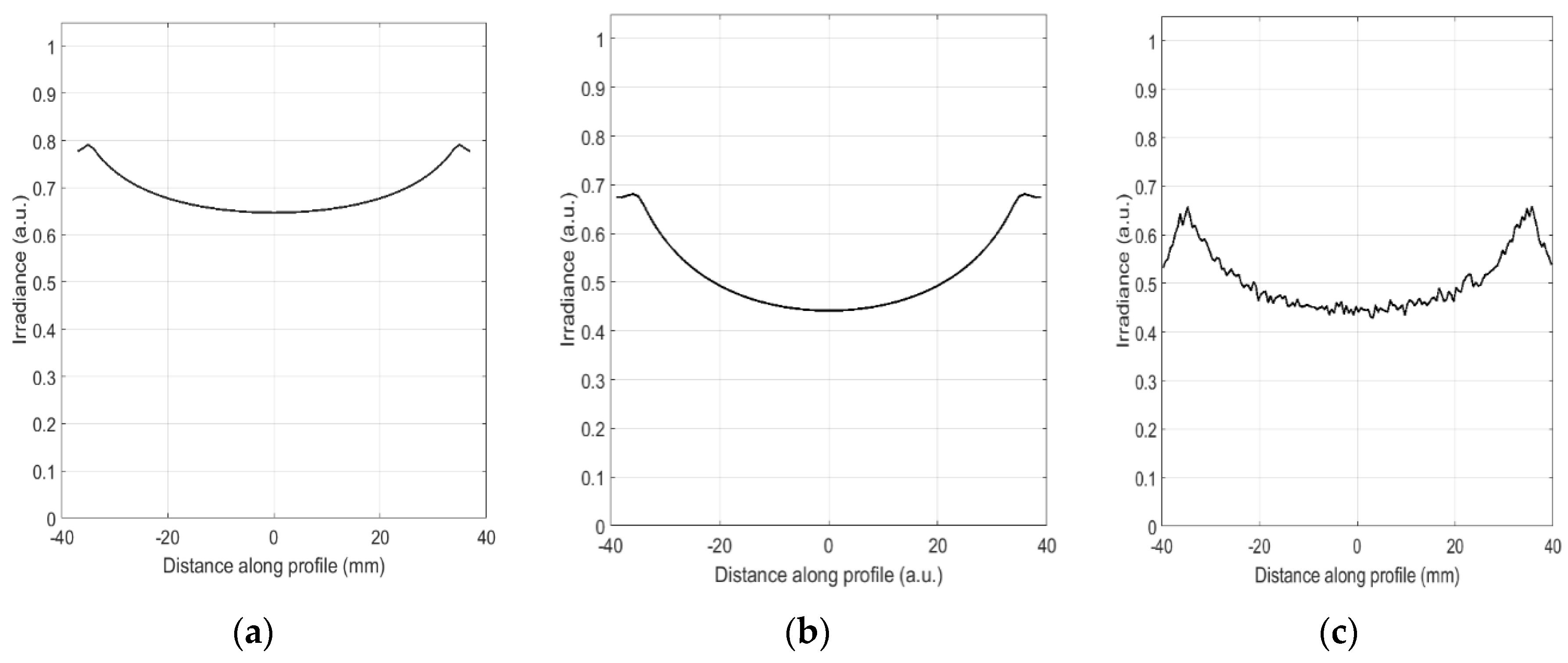
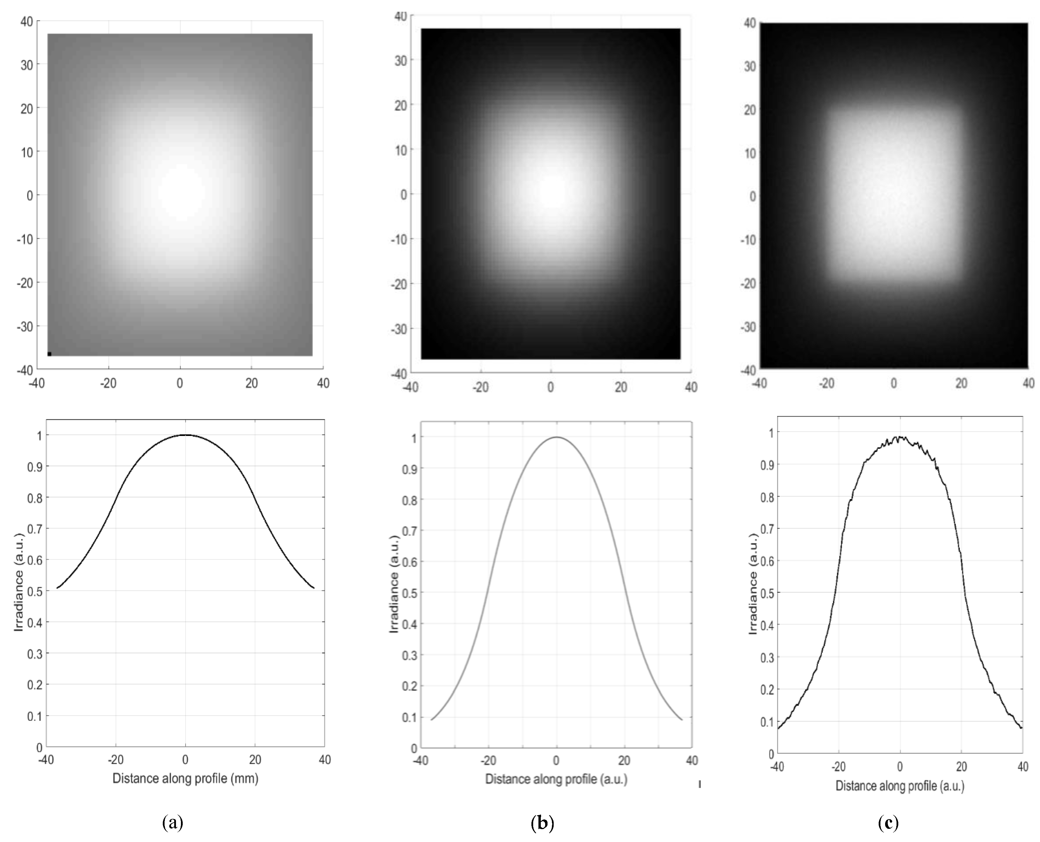
3. Irradiance Computation from J Vector for Asymmetric 3D Systems with Refractive Elements

As the next step in the development of a vector potential flowline technique for optical simulation, we analyzed a simple 3D refractive system consisting of a square source, a plano-convex lens and a detector. Figure 5 shows a sketch of the analyzed system. We computed the vector potential A at the position of the detector by replacing the distance r in Equation (3) with optical path length (OPL), L. This introduced a new challenge in the computation of the contour integral of Equation (3). Before calculating the integral value at any point in the detector, such as point P, it is necessary to compute the optical path length between point P and all the points in the closed contour of the source C. In this way, the irradiance E at point P on the detector for the system of Figure 5 with Lambertian source can be computed from the contour source integral to Equation (3) with the log of OPL and the derivatives of Equation (4). It is possible to do so using Fermat’s principle. We developed some routines in Matlab based on Nelder–Mead minimum algorithm to compute the OPL for this simple optical system. Another option was to use the routines incorporated in the Raytracer package software, which includes the computation of OPL. Once we computed the OPL between one point in the detector and the closed contour of the source, it was then possible to compute the vector potential A at any point in the detector from the integral of Equation (3). Finally, we obtained the irradiance pattern E at detector from A following Equation (4). Figure 5 shows a sketch of the analyzed optical system. A Lambertian square source of 10 mm side was located at the origin, and a plano-convex lens was located at z = 300 mm (plane size of the lens). The convex surface of the lens had a radius R = 150 mm, the thickness of the lens at the axis was 30 mm, the refraction index was n = 1.5, and the lens had a square perimeter of 120 mm per side. Finally, there was also a square detector of 80 mm per side, located at z = 950 mm.

Figure 6 demonstrates the comparison between flow line vector potential and the results obtained by raytrace. Figure 6a shows the irradiance pattern and the corresponding profiles of flowline computation, and column Figure 6b shows the irradiance pattern and corresponding profiles of raytrace computation. It can be seen that there was a partial agreement between the two computation methods. The flowline method accurately predicted the position of maximum and minimum irradiance patterns at the detector; however, there were disagreements in the irradiance values of these local maximums and minimums, as shown in the irradiance profiles of Figure 6a,b.

From the analysis of these results, it appears clear that the vector potential theoretical model needs correction to match the raytrace results. However, it is interesting that the standard vector potential method was capable of predicting the position of the maximum in the irradiance pattern. This suggests that the right model must be close to the standard vector potential method, and some changes will be needed in order to achieve complete agreement between flowline and raytrace simulations.

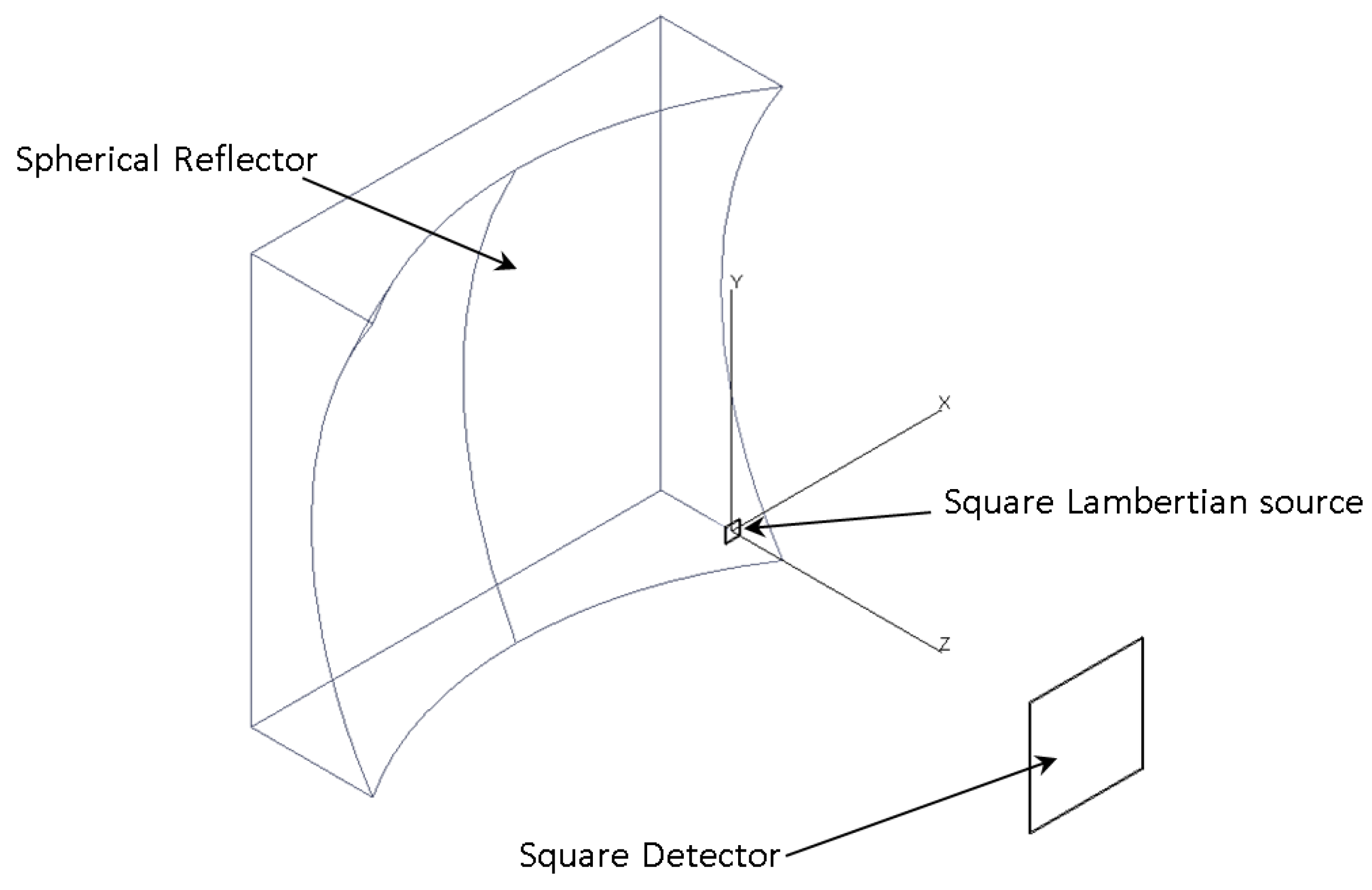
4. Irradiance Computation from J Vector for Asymmetric 3D Systems with Reflective Elements

To advance the development of the flowline 3D optical simulation technique, we completed our study with the analysis of a simple asymmetric reflective system. Figure 7 shows the sketch of a reflective system, composed of a square source; a spherical reflector with its center in the optical axis (OZ axis) with a square perimeter; and a detector, which was also square. In this case, the light source emitted light in the –OZ direction (directly towards the reflective surface). No direct light from the source was received by the detector. We studied several configurations that produced both the maximum and the minimum of irradiance at the detector surface. The details are as follows: First, we studied a perfect mirror surface of R = 300 mm, with the center located at z = 110 mm; the source was a square Lambertian source of 10 mm per side, located at the origin of the reference system; there was also a square detector of 80 mm per side located at z = 250 mm. Figure 8 demonstrates the normalized irradiance pattern of this configuration, and Figure 9 shows the central irradiance profiles from this configuration, from flowline computation and also from raytrace computation.

Second, we analyzed different irradiance patterns for the same reflective system, moving the detector to z = 550 mm. With this change, the irradiance distribution obtained by raytrace had a central maximum which was close to the shape of a square. As we have previously mentioned for this configuration, it was necessary to compute the vector potential using Equation (3), and to do that, we needed to first compute the optical path length. We therein chose the Nelder–Mead algorithm for this computation. The interesting result found was that for this latest configuration (z = 550 mm), the OPL was obtained as the maximum of Fermat principle, although for previous configuration the OPL was obtained as the minimum of Fermat principle. Figure 10 shows the normalized irradiance pattern and Figure 11 shows the central irradiance profile comparisons. For reflective optical systems, the vector potential method produced a similar irradiance pattern compared with the refractive system, with well-located maxima and minima, but the magnitude appeared to be different between the flowline and the raytrace computations. In the next section, we propose a correction to the vector potential method in order to correct these differences.

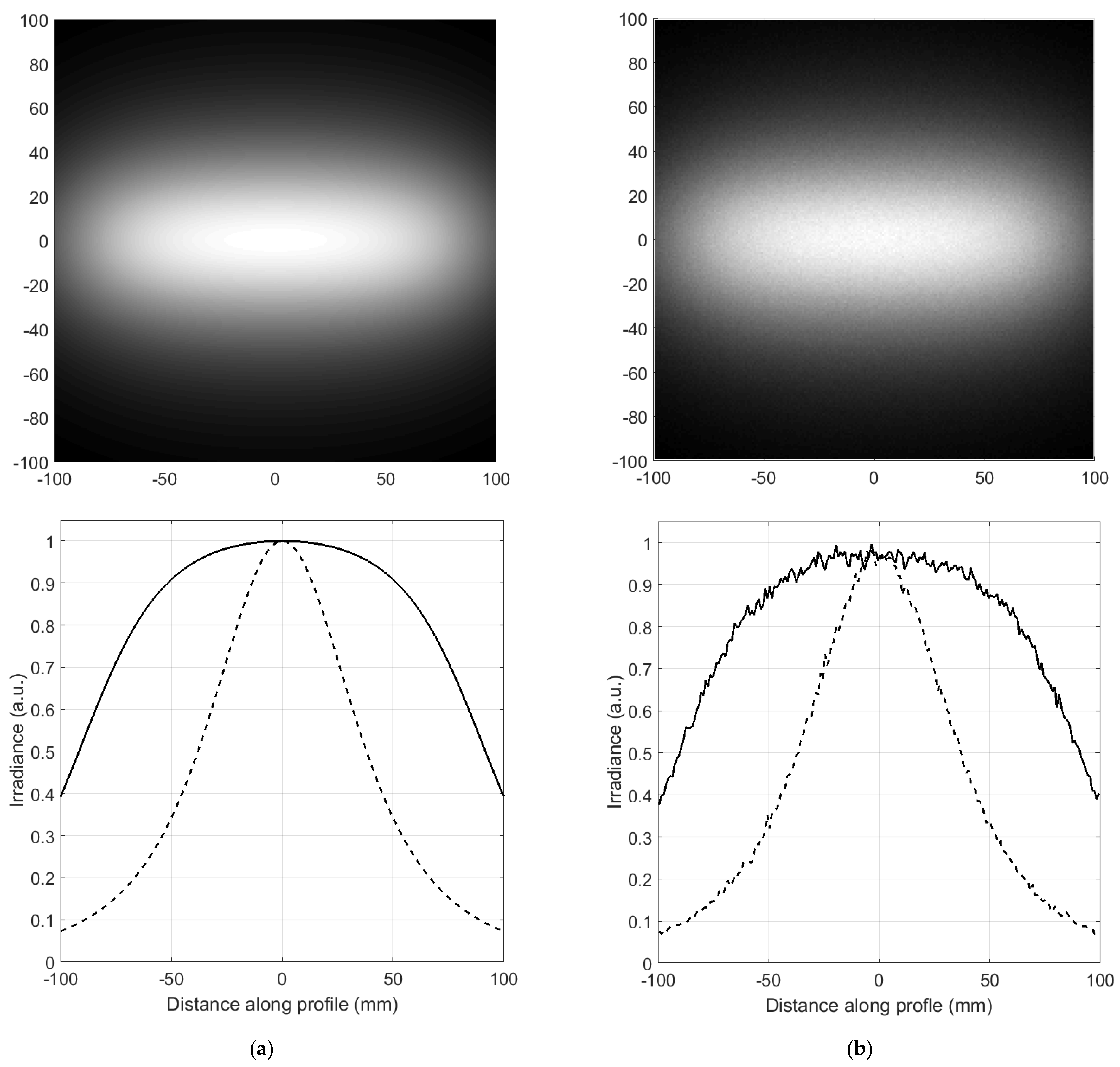
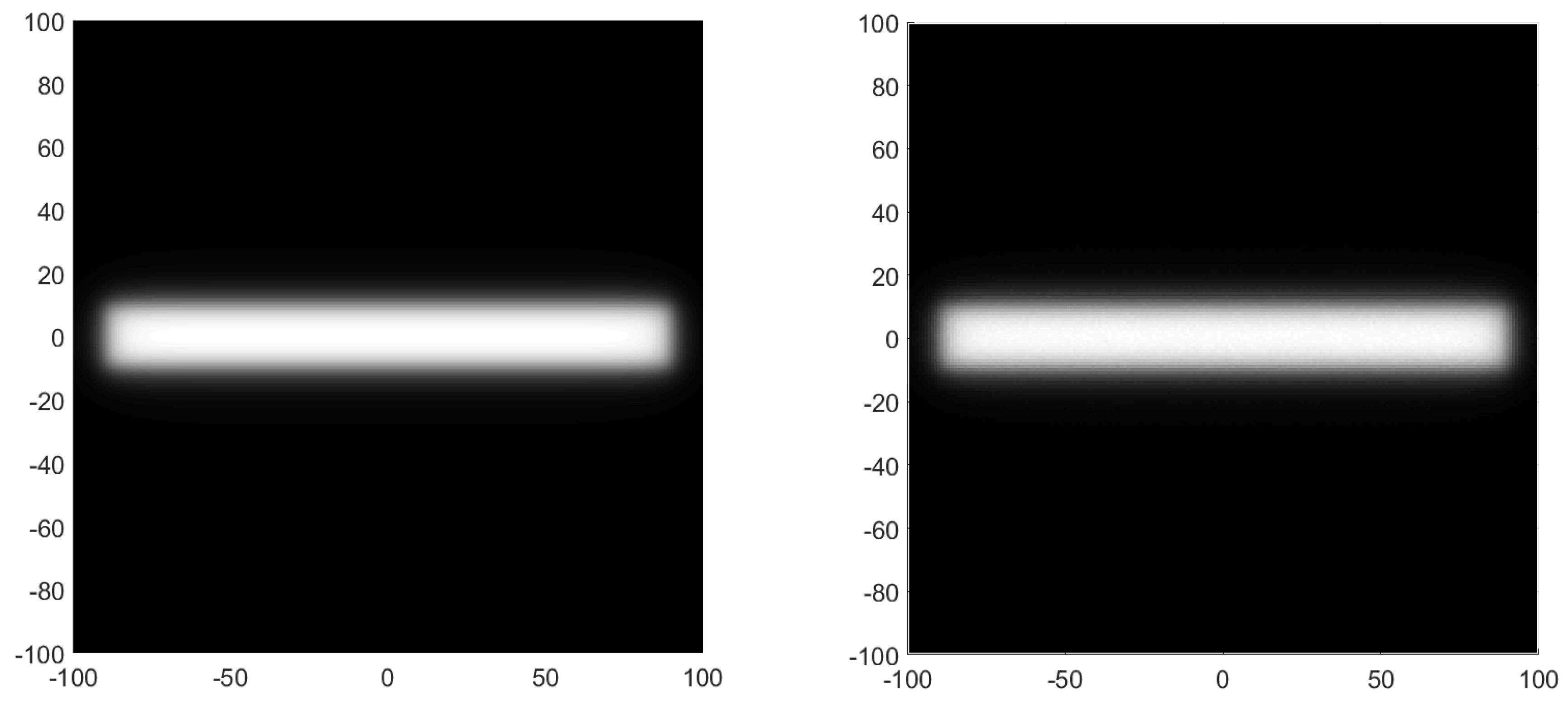
5. Optical Path Length Correction for Standard Vector Potential Method

A gauge transformation can be understood as a transformation with some degree of internal freedom, one that does not modify any direct observable physical property. As an example, we can always choose a scalar potential by adding a constant or a vector potential by adding the gradient of a scalar function [11]. Jiang and Winston [12] suggested that vector potential for 2D optical systems can be calculated from the optical path length difference and a constant. They demonstrated that for 2D compound elliptical concentrator (CEC), the adding constant is needed for vector potential calculations at the border of regions for CEC design. Following that idea, we proposed a correction to the standard vector potential model by introducing a constant λ into the optical path length definition, L′. This is similar to the gauge transformation by adding a constant to scalar potential,

$$L^{\prime }={\displaystyle \sum }_i{n}_i{s}_i+\lambda$$

(5)

where n_i is the refractive index, s_i is the distance of the ray along the optical media, and λ is a constant. This transformation of the optical path length is fully compatible with Fermat’s principle. All classical consequences of Fermat’s principle remain unaltered. We also proposed that the vector potential can be computed by the integral of Equation (3) by replacing the distance r with the proposed corrected optical path length L′.

We have checked the proposed correction term in Equation (5) for the refractive system of Section 3 and the reflective configurations shown in Section 4. Figure 12b shows the correction produced by introducing constant λ in the refractive system of Section 3, and the fit between raytrace and the corrected flowline method was obtained by λ = 945 mm. Figure 13 shows non-corrected flowline computation in sub-figure (a) and corrected flowline computation in sub-figure (b). The raytrace result is shown in Figure 13c for the reflective system, with the detector located at z = 250 mm. The correction factor took the value λ = 605 mm. Finally, Figure 14 shows non-corrected flowline computation in sub-figure (a), and corrected flowline computation in sub-figure (b). The raytrace computation is shown in Figure 14c for the reflective system, with the detector located at z = 550 mm. The correction factor took the value λ = 926 mm. All analyzed configurations, both refractive (Figure 12) and reflective (Figure 13 and Figure 14), showed a better fit. Second order differences between flowline and raytrace still remain, for example, the boundaries of the irradiance pattern (Figure 12), sampling, number of rays traced, or further corrections to flowline method can be studied for better agreement. The correction parameter λ was close to the maximum optical path length. The L′ was greater than 1, but L′ << L; the theoretical meaning of this correction still needs new investigation and study, but we can intuitively suggest that it comes from the fact that the definition of vector potential A in Equation (2) is not unique. The gradient of a scalar function can be always added to A with Equation (2) remaining unaltered, which is in agreement with gauge transformation.

6. Conclusions

In this paper, we analyzed the vector potential A of flowline vector J. We applied this analysis to non-axisymmetric refractive and reflective optical systems. As prescribed by the theoretical method, we replaced the standard distance r by classical optical path length L. With this replacement, we obtained interesting results, such as the precise location of irradiance maximum in the distribution. However, this method seems to need corrections to obtain agreement between raytrace simulations and the vector potential of J vector computations. We then proposed a corrected version of the optical path length L′ by introducing a constant parameter, which was similar to the gauge invariant. This corrected version of the optical path length is compatible with the Fermat principle, and provided better agreement between the raytrace simulations and the vector potential computations. Nevertheless, the study of the physical meaning of this corrected optical path length L′ remains an open question.

References

1. Gershun, A. The light Field. J. Math. Phys. 1939, 18, 51–151. [Google Scholar] [CrossRef]
2. Moon, P.; Spencer, D.E. Photic Field; Massachusetts Institute of Technology Press: Cambridge, MA, USA, 1981. [Google Scholar]
3. Winthrop, J.T. Propagation of Structural Information in Optical Wave Fields. J. Opt. Soc. Am. 1971, 61, 15–30. [Google Scholar] [CrossRef]
4. Winston, R.; Welford, W.T. Geometrical vector flux and some new nonimaging concentrators. J. Opt. Soc. Am. 1979, 69, 532–536. [Google Scholar] [CrossRef]
5. Winston, R.; Welford, W.T. Ideal flux concentrators as shapes that do not disturb the geometrical vector flux field: A new derivation of the compound parabolic concentrator. J. Opt. Soc. Am. 1979, 69, 536–539. [Google Scholar] [CrossRef]
6. Welford, W.T.; Winston, R. High Collection Nonimaging Optics; Academic Press: San Diego, CA, USA, 1989. [Google Scholar]
7. García-Botella, A.; Fernández-Balbuena, A.A.; Vázquez, D.; Bernabeu, E.; González-Cano, A. Hyperparabolic Concentrators. Appl. Opt. 2009, 48, 712–715. [Google Scholar] [CrossRef] [PubMed]
8. García-Botella, A. Ideal flux field dielectric concentrators. Appl. Opt. 2011, 50, 5357–5360. [Google Scholar] [CrossRef] [PubMed]
9. García-Botella, A.; Jiang, L.; Winston, R. Optical simulation-based on flowline method. In Proceedings of the SPIE, Nonimaging Optics: Efficient Design for Illumination and Solar Concentration XV, San Diego, CA, USA, 19–23 August 2018. [Google Scholar]
10. Tracepro Software. Available online: http://www.lambdares.com/ (accessed on 28 September 2019).
11. Landau, L.D.; Lifschitz, E.M. The Classical Theory of Fields; Pergamon Press: Oxford, UK, 1971. [Google Scholar]
12. Jiang, L.; Winston, R. Flowline design and thermodynamic implications of the vector potential. In Proceedings of the SPIE, Nonimaging Optics: Efficient Design for Illumination and Solar Concentration XV, San Diego, CA, USA, 19–23 August 2018. [Google Scholar]
Figure 1. Sketch of the 3D analyzed system of non-symmetric source.
Photonics 06 00101 g001
Figure 2. Irradiance map and central irradiance profile of square source of 160 × 160 mm2; detector of 200 × 200 mm2; z detector distance 20 mm. (a)Flowline computation (b) Raytrace computation
Photonics 06 00101 g002
Figure 3. Irradiance map and central irradiance profile of rectangular source of 20 × 180 mm2; detector of 200 × 200 mm2; z detector distance 5 mm. (a) Flowline computation (b) Raytrace computation
Photonics 06 00101 g003aPhotonics 06 00101 g003b
Figure 4. Irradiance map and central irradiance profile of rectangular source of 20 × 180 mm2; detector of 200 × 200 mm2; z detector 50 mm. (a)Flowline computation (b) Raytrace computation
Photonics 06 00101 g004
Figure 5. Sketch of the 3D source-lens-detector analyzed system.
Photonics 06 00101 g005
Figure 6. Irradiance pattern and central irradiance profile at the detector: (a) computed by flowline vector potential method; (b) computed by raytrace.
Photonics 06 00101 g006
Figure 7. Sketch of the analyzed 3D reflective optical systems.
Photonics 06 00101 g007
Figure 8. Normalized irradiance pattern of reflective system, detector at z = 250 mm: (a) flowline computation; (b) raytrace computation.
Photonics 06 00101 g008
Figure 9. Central irradiance profile of distributions of Figure 8: (a) flowline computation; (b) raytrace computation.
Photonics 06 00101 g009
Figure 10. Normalized irradiance pattern of reflective system, detector located at z = 550 mm: (a) flowline computation; (b) raytrace computation.
Photonics 06 00101 g010
Figure 11. Central irradiance profile of distributions of Figure 10: (a) flowline computation; (b) raytrace computation.
Photonics 06 00101 g011
Figure 12. Irradiance pattern and central irradiance profile at the detector for refractive optical system of Section 3: (a) computed by standard flowline vector potential method; (b) computed by optical path length (OPL) correction in flowline vector potential method; (c) computed by raytrace.
Photonics 06 00101 g012
Figure 13. Irradiance pattern and central irradiance profile at the detector for the reflective system, with the detector located at z = 250 mm: (a) computed by standard flowline vector potential method; (b) computed by OPL correction in flowline vector potential method; (c) computed by raytrace.
Photonics 06 00101 g013aPhotonics 06 00101 g013b
Figure 14. Irradiance pattern and central irradiance profile at the detector for the reflective system with the detector located at z = 550 mm: (a) computed by flowline vector potential method; (b) computed by OPL correction in flowline vector potential method; (c) computed by raytrace.
Photonics 06 00101 g014