The Theoretical Concept of Polarization Reflectometric Interference Spectroscopy (PRIFS): An Optical Method to Monitor Molecule Adsorption and Nanoparticle Adhesion on the Surface of Thin Films

Abstract

In this paper, we present an improved reflectometric interference spectroscopy (RIfS) sensor principle which is suitable for thin films. The conventional RIfS technique is an appropriate method to detect interfacial interactions at the solid–gas or solid–liquid interface in the case of thin films with a thickness of a few hundred nanometers, but when a significantly lower layer thickness (~100 nm) is required, the method is barely usable. By applying polarized reflected light and monitoring the ratio of the p- and s-polarized components, a characteristic curve can be obtained with one or a few local extreme value(s) with significantly favorable intensity ratios compared to the conventional method. In this work we studied the effect of film thickness, incident angle and the refractive indices of the thin film, the medium and the substrate. As a main result, it was demonstrated that the sensitivity of the PRIfS method is 4–7 times higher than that of the conventional technique near a critical angle. In simulated adsorption experiments, it was determined that the sensitivity of RIfS is around 550 nm/RIU (refractive index unit), while it is 1825 and 3966 nm/RIU for PRIfS in gas and aqueous phase, respectively.

1. Introduction

The monitoring of molecule adsorption or nanoparticle adhesion on different surfaces is based on the measurement of the surface excess. Several methods are known in the literature to detect the presence of any adsorbate: electric (resistive [1,2,3] and capacitive [4,5]) techniques operate mainly in the gas phase as volatile organic compound (VOC) sensors [6,7], while optical methods can be used both in gas and aqueous medium, mainly as biosensors. The latter group can be divided into plasmonic [8,9,10], waveguide [11,12] and reflectometric devices.

Reflectometric interference spectroscopy is an optical method suitable for thin film characterization [13,14,15,16], as well as for sensorial applications in aqueous [17,18] and gas phase [6,19,20]. The RIfS technique is based on the spectral shift of the interference pattern of Fabry-Perot fringes reflected from thin films with a few hundred nanometers of layer thickness. The wavelength shift is caused by the adsorption or adhesion of molecules or nanoparticles, and thus it is applicable as a biosensor or VOC sensor. The advantage of this technique is the extensive detection layer: it can be up to a few hundred nanometers, making it capable of the detection of bacteria or cells, for example [21,22]. However, the drawback of the method is that a relatively high film thickness (200–600 nm) is required to obtain the interference pattern [23,24,25,26,27,28], mainly in the case of FT-RIfS (Reflective Interferometric Fourier Transform Spectroscopy), where the sensing layer (substrate) is highly ordered nanoporous anodic aluminum oxide (AAO) with a layer thickness of a few micrometers [22,29,30]. By using high refractive index materials (e.g., SiN), the thickness of the sensing layer can be slightly reduced [31,32,33].

In this work, we made an attempt to examine the application of polarized light for reducing the sensing layer thickness, even in the case of low refractive index materials. Compared to the conventional RIfS technique, a polarizer is used in front of the detector, and in this manner only the p- or s-polarized component of the reflected light reaches the detector. We also demonstrated detailed calculations about how the film thickness, the angle of incidence and the refractive index of the thin film, the substrate and the medium affect the shape and intensity conditions of the calculated curves, which are the ratio of the p- and s-polarized components of the reflected light. Furthermore, we demonstrated through simulated adsorption experiments that the sensitivity of the PRIfS curve is four to six times higher than the conventional RIfS method near a critical angle: the sensitivity of RIfS is around 550 nm/RIU, while it is 1825 and 3966 nm/RIU for PRIfS in gas and aqueous phase, respectively. A further study of the experimental implementation of the method can substantiate our results.

2. Methods

The conception of the polarization reflectometric interference spectroscopy (PRIfS) method is similar to the conventional RIfS technique, the difference lies only in the implementation of the measurement. Figure 1 shows the schematic diagram of a typical reflectometric setup (with a polarizer) and calculation of the most notable parameters:

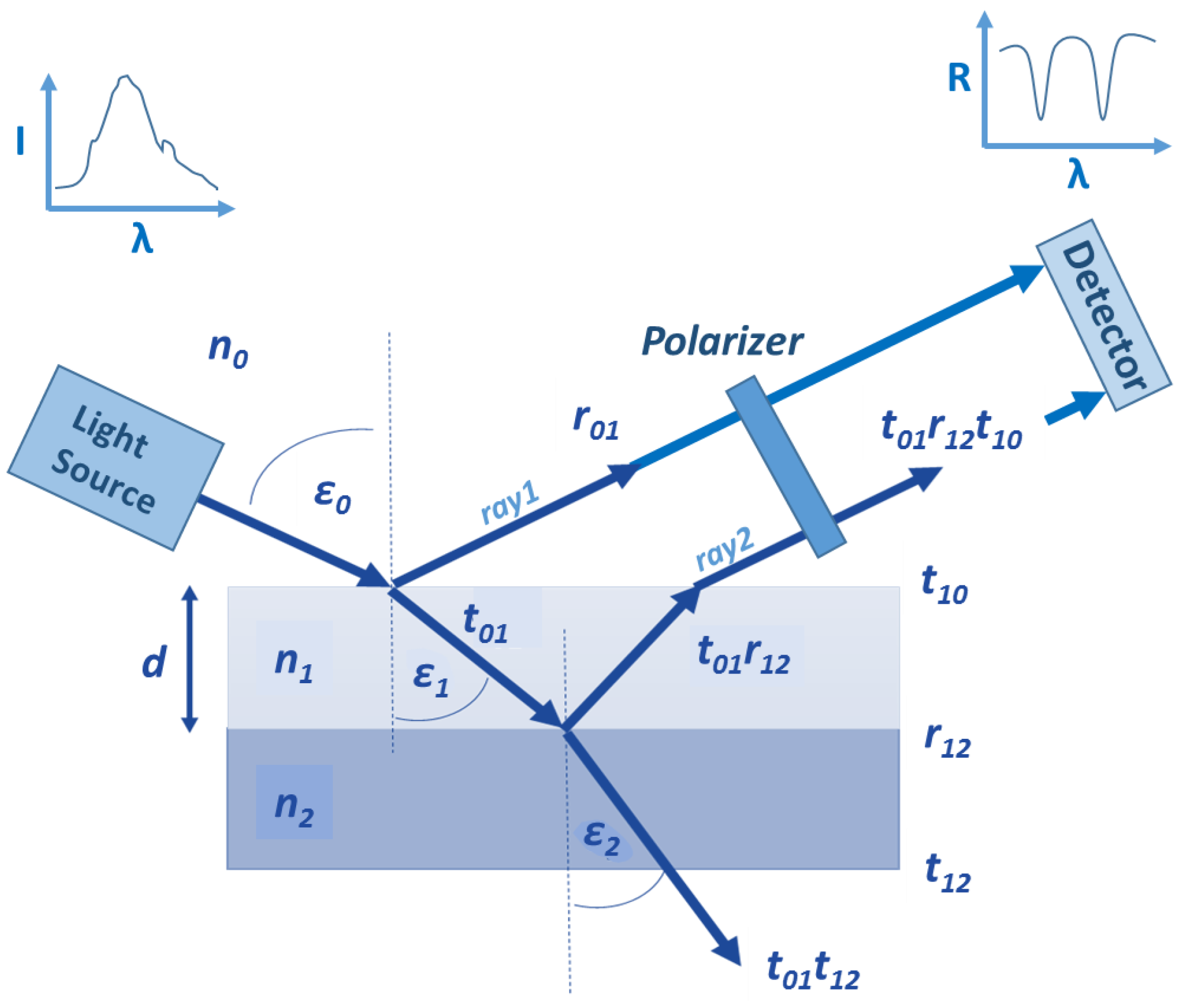
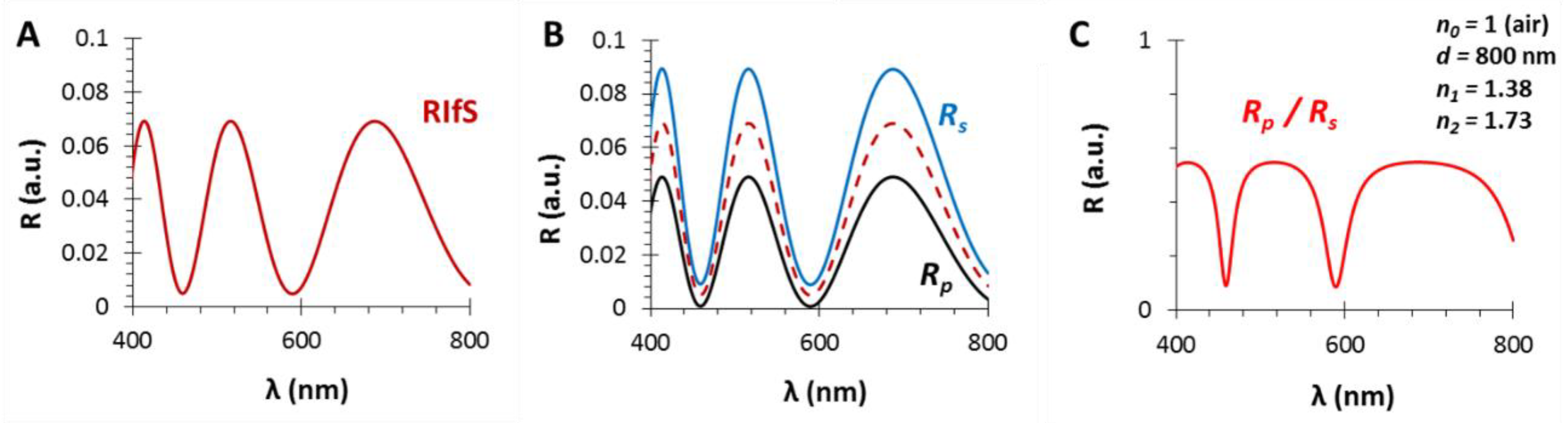
2.1. The Reflectometric Interference Spectroscopy Principle

In the case of the conventional RIfS method, the reflected intensity from a thin film can be calculated by the complex amplitude method [15]. The intensity is proportional to the square of the amplitude:

$$I_R~A^2=\left(A·e^{i\theta }\right)\left(A·e^{-i\theta }\right)$$

(1)

where the complex amplitude is (see notations on Figure 1, ray1 and ray2):

$$A·e^{i\theta }=a·r_{01}+a·t_{01}{r}_{12}{t}_{10}·e^{i\delta }$$

(2)

δ is the phase difference between the two rays (ray1 and ray2), which can be expressed by the optical path length difference (Δ):

$$\delta =\frac{2\pi }{\lambda }\Delta =\frac{2\pi }{\lambda }·2n_{1}d·cos{\epsilon }_1$$

(3)

where d is the thin film thickness and λ is the wavelength. We note that there is an exp(iπ) phase shift at the air/film interface, as well as at the film/substrate phase boundary, if n₂ > n₁, and the resultant of the double phase shift is zero. The reflection and transmission amplitude parameters in Equation (2) can be calculated by the following equations:

$$r_{ij}=\frac{n_i-n_j}{n_i+n_j}$$

(4)

$$t_{01}=1-r_{01}$$

(5)

$$t_{10}=\frac{1-r_{01}^2}{t_{01}}$$

(6)

The reflected intensity from the surface of a thin film is described by Equation (7):

$$I_R~r_{01}^2+r_{12}^2{\left(1-r_{01}^2\right)}^2+2r_{01}{r}_{12}{\left(1-r_{01}\right)}^{2}cos\left(\frac{4\pi n_{1}d·cos{\epsilon }_1}{\lambda }\right)$$

(7)

This equation describes a typical reflectometric interference spectrum decorated with the interference pattern of Fabry-Perot fringes (see Figure 2A). Equations (4)–(6) show that the calculation ignores the polarization effect.

2.2. The Polarization Reflectometric Interference Spectroscopy Principle

In the case of the polarization reflectometric interference principle, the r₀₁, r₁₂, t₀₁ and t₁₂ amplitudes are calculated in different ways depending on the polarization state (s: senkrecht and p: parallel) [34].

$$r_{ij,s}=\frac{n_i\cos \left({\epsilon }_i\right)-n_j\cos ({\epsilon }_j)}{n_i\cos \left({\epsilon }_i\right)+n_j\cos \left({\epsilon }_j\right)}$$

(8)

$$r_{ij,p}=\frac{n_j\cos \left({\epsilon }_i\right)-n_i\cos ({\epsilon }_j)}{n_j\cos \left({\epsilon }_i\right)+n_i\cos \left({\epsilon }_j\right)}$$

(9)

$$t_{ij,s}=\frac{2n_i\cos \left({\epsilon }_i\right)}{n_i\cos \left({\epsilon }_i\right)+n_j\cos \left({\epsilon }_j\right)}$$

(10)

$$t_{ij,p}=\frac{2n_i\cos \left({\epsilon }_i\right)}{n_j\cos \left({\epsilon }_i\right)+n_i\cos \left({\epsilon }_j\right)}$$

(11)

The equations clearly show that the technique is limited to oblique incidence (ε₀ > 0°), otherwise the reflection amplitudes in Equations (7) and (8) become equal to each other and to the coefficient in Equation (4) and the polarization effect ceases (see Figure A1b). These reflection amplitude values are included in the I_R equations, similarly to in Equation (7):

$$I_{R,s}~r_{01,s}^2+r_{12,s}^2{\left(1-r_{01,s}^2\right)}^2+2r_{01,s}{r}_{12,s}{\left(1-r_{01,s}\right)}^{2}cos\left(\frac{4\pi n_{1}d·cos{\epsilon }_1}{\lambda }\right)$$

(12)

$$I_{R,p}~r_{01,p}^2+r_{12,p}^2{\left(1-r_{01,p}^2\right)}^2+2r_{01,p}{r}_{12,p}{\left(1-r_{01,p}\right)}^{2}cos\left(\frac{4\pi n_{1}d·cos{\epsilon }_1}{\lambda }\right)$$

(13)

The difference between the RIfS and PRIfS methods lies in the measurement techniques. While the detector measures the average of all the polarization states in the former case, the ratio of the s- and p-polarized reflected intensity is measured by using a polarizer in the latter (Equation (14)).

$$I_{R,PRIfS}=I_{R,p}/I_{R,s}$$

(14)

This difference is illustrated on Figure 2: (A) is a conventional RIfS spectrum, (B) presents the s- and p-polarized spectra and their average, whereas (C) shows the ratio of the s- and p-polarized components of the spectrum (when the thickness and refractive index of the thin film are d = 800 nm and n₁ = 1.38, respectively, using a substrate with n₂ = 1.7, in air, ε₀ = 35°).

3. Results and Discussion

The difference between the conventional and polarized RIfS techniques was demonstrated by Equations (7), (12)–(14). It is clear that the reflected intensity pattern (I_R) depends on several explicit and implicit parameters which are included in the components of the summation. While the explicit parameters are the film thickness (d), the refraction angle (ε₁) and the refractive index of the film (the sensing layer) (n₁), the implicit parameters are included in the reflection and transmission amplitudes (in conventional and polarized cases, Equations (4)–(6), (8)–(11), respectively), namely the refractive indices of the medium (n₀), the film (n₁) and the substrate (n₂). The dependence of the reflected intensity on these parameters are demonstrated in Section 3.1, Section 3.2 and Section 3.3, while two simulated, time-resolved adsorption experiments are presented in Section 3.4 and Section 3.5.

Considering that the RIfS curve is the average of all the polarization states, therefore RIfS, R_s and R_p curves are hardly different (see Figure 2A,B) (except near the Brewster angle, where R_p ≈ 0, see Figure A1, Figure A2, Figure A3 and Figure A4 in Appendix A), only the R_S and R_P curves are shown in Figure 3, Figure 4 and Figure 5 for the sake of visual clarity. For similar reasons, the refractive indices of the thin film and the substrates are indicated as constant values (average value in the λ = 400–800 nm wavelength range); however, in the calculations, the characteristic n₂(λ) (dispersion) functions are used (fused silica [35] and SF10 [36] glasses). Assuming that the thin film materials are weakly or non-absorbent in the investigated (visible) wavelength range (e.g., ZnO, TiO₂), the refractive indices of the thin films are considered to be real. In the case of absorbing materials, the refractive index should be extended to the complex value (η), introducing k as the extinction coefficient (η = n + ik). On the other hand, it should be noted that the low effective refractive index (RI) value (1.1 < n₁ < 1.6) is a typical feature in the case of polymer or porous nanostructured thin films in sensorial applications, while the higher RI values are characteristic to sputtered layers, for example in antireflective and low-E coatings.

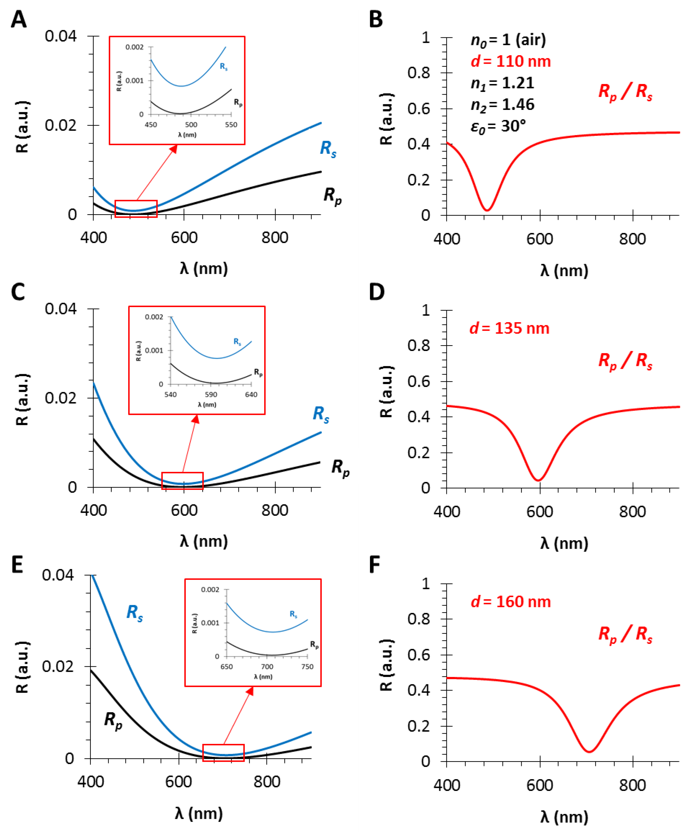
3.1. The Film Thickness (d)

Figure 3 shows the calculated reflectance curves from a thin film with an effective refractive index of n₁ = 1.21 and different film thicknesses, d = 110, 135 and 160 nm (Figure 3A,B, Figure 3C,D and Figure 3E,F, respectively).

The angle of incidence is ε₀ = 30°, the RI of the medium is n₀ = 1 (gas phase) and the model substrate is fused silica glass (n₂ = 1.46), since these are typical gas phase VOC sensor conditions [6], except the low layer thickness which is much lower than the suitable value in RIfS technique. It can be observed in Figure 3A,C,E that the interference pattern barely appears because of the low sensing layer thickness, compared to Figure 2B (d = 800 nm). In contrast, when the ratio of the s- and p-polarized components is measured, the obtained reflectance curve has a definite extreme value (edge). These curves (corresponding to different layer thicknesses) have the similar shape, contrast and FWHM (full width at half maximum) with the increase in layer thickness d, while only the edge shifts toward the higher values (red shift) (see Figure 3B,D,F). The wavelength shift, and thereby the wavelength of the edge can be precisely tuned: the scaling factor is λ/d = 4.5 nm/nm.

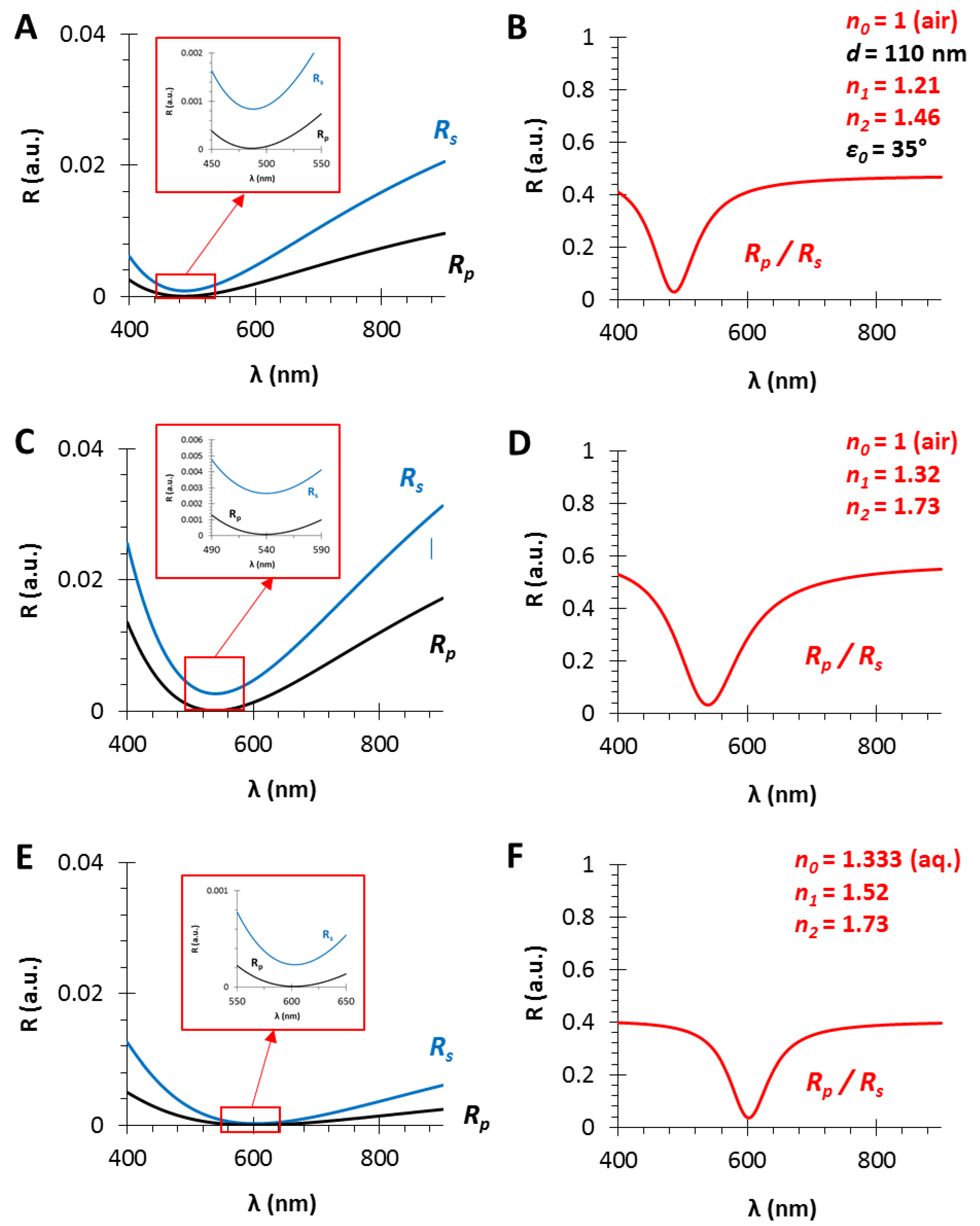
3.2. The Refractive Index of the Medium (n₀), the Thin Film (n₁) and the Substrate (n₂)

In Section 3.1, it was presented that the shape of the PRIfS curve does not vary with the increase in layer thickness d, only the corresponding wavelength of the edge shows a red shift. In contrast, if the refractive index of the medium, the sensing layer or the substrate are varied, then both the wavelength of the edge and the intensity contrast (FWHM) also change (Figure 4).

It has to be noted that the optimal refractive index matching condition is the geometric mean between the refractive indices of the medium and the substrate. Three optimal cases are presented in Figure 4: in the gas phase (n₀ = 1), the optimal thin film refractive index is n₁ = 1.21 when fused silica substrate (n₂ = 1.46) is used (Figure 4A,B). Similarly, n₁ = 1.32 or n₁ = 1.52 thin film refractive indices are the optimal values in the case of SF10 substrate in air (Figure 4C,D) or in aqueous phase (Figure 4E,F), respectively. Furthermore, it can be observed that the contrast and the FWHM of the curves are determined by the refractive index difference between two adjacent media (n_i and n_j in Equation (4), which can be n₀ and n₁, or n₁ and n₂, as the refractive indices of the medium and the thin film, or the thin film and the substrate, respectively). It can be established that the higher refractive index difference results in greater contrast (ΔR = 0.55) and FWHM (Δλ = 100 nm), when the R_S and R_P curves are almost parallel in the region of interest (see Figure 4C, zoom), compared to the lower RI difference with diverging R_S and R_P curves (ΔR = 0.4 and Δλ = 70 nm, Figure 4B,D). The further advantage of the proper RI matching, i.e., the geometric mean, is that the Brewster angle (Θ_B) will be the same at the medium/film and film/substrate interfaces [Θ_B = arctan(n₁/n₀) = arctan(n₂/n₁)]. In Section 3.4 and Section 3.5, these optimal conditions will be examined in simulated absorption experiments: for sensorial measurements in gas phase, thin films with low refractive index are applicable, while in aqueous phase a relatively high (n₁~1.5) RI is required. The RI increase can be achieved by applying materials with higher refractive index (e.g., SiN, TiO₂) or by decreasing the porosity of the sensing layer.

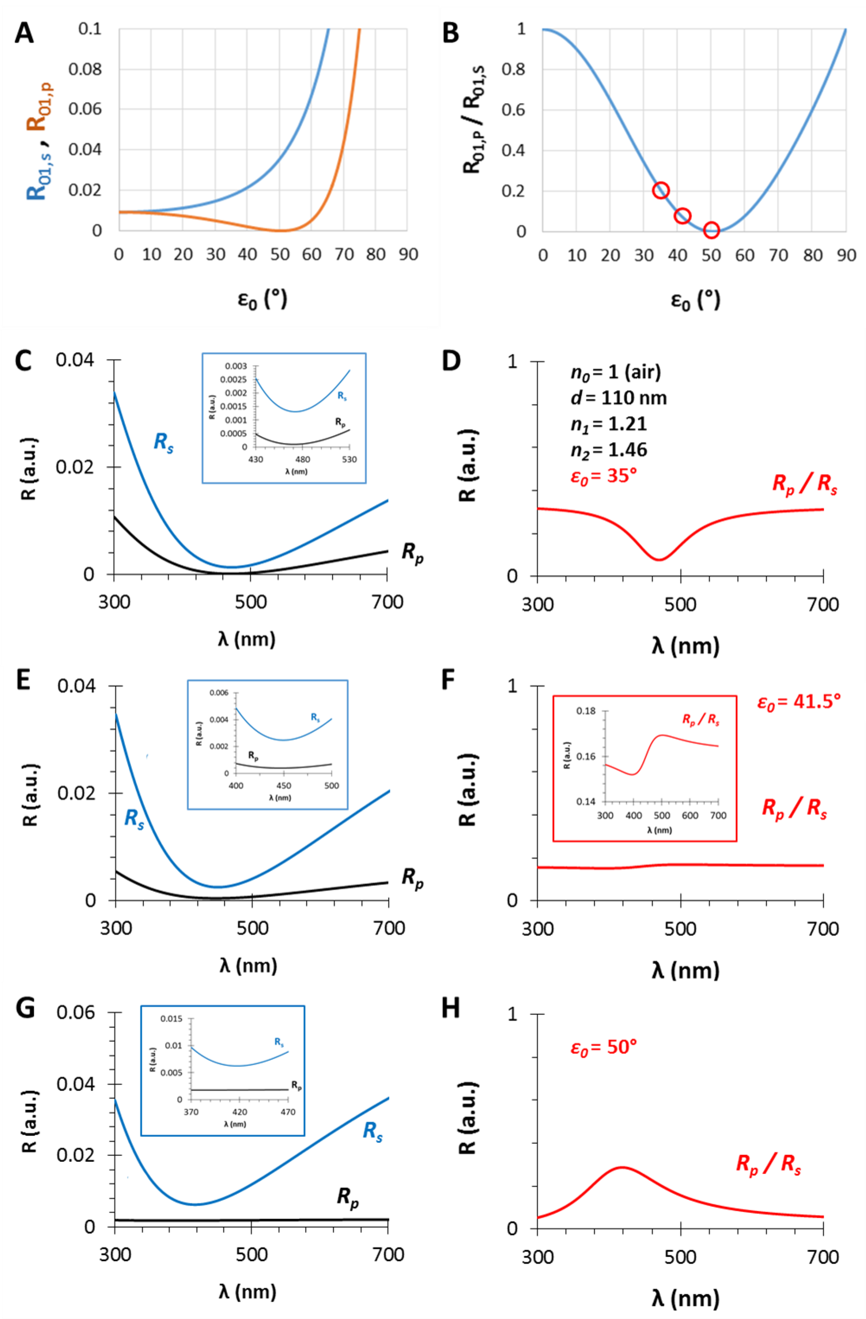
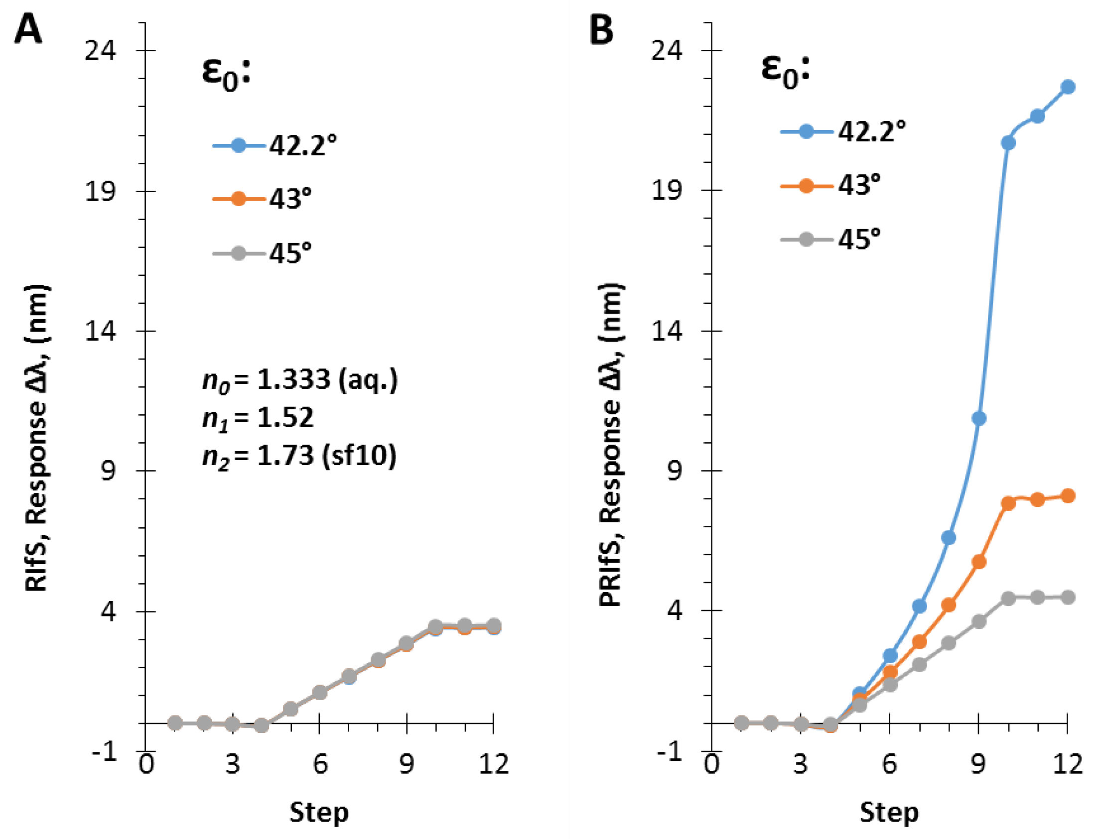
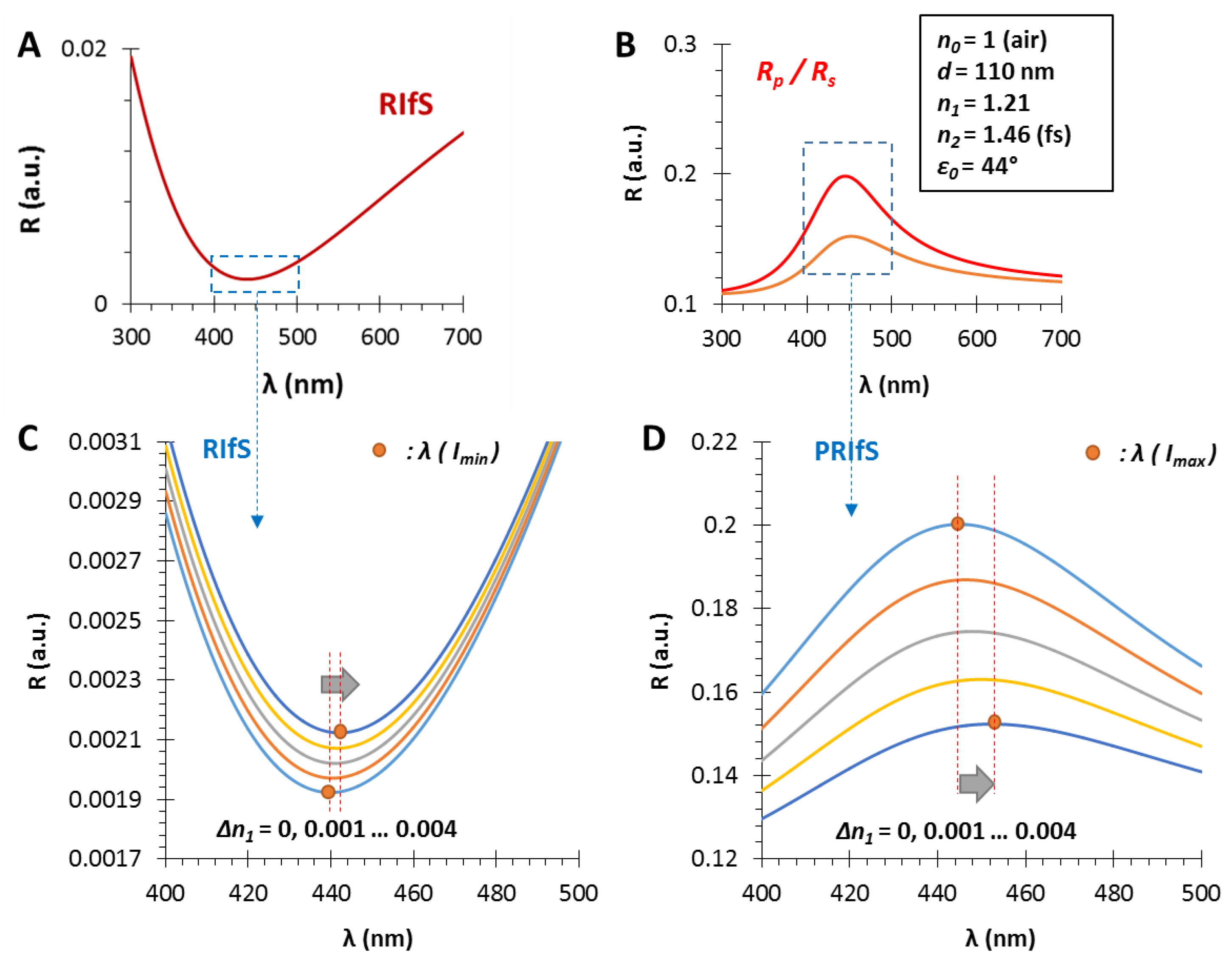
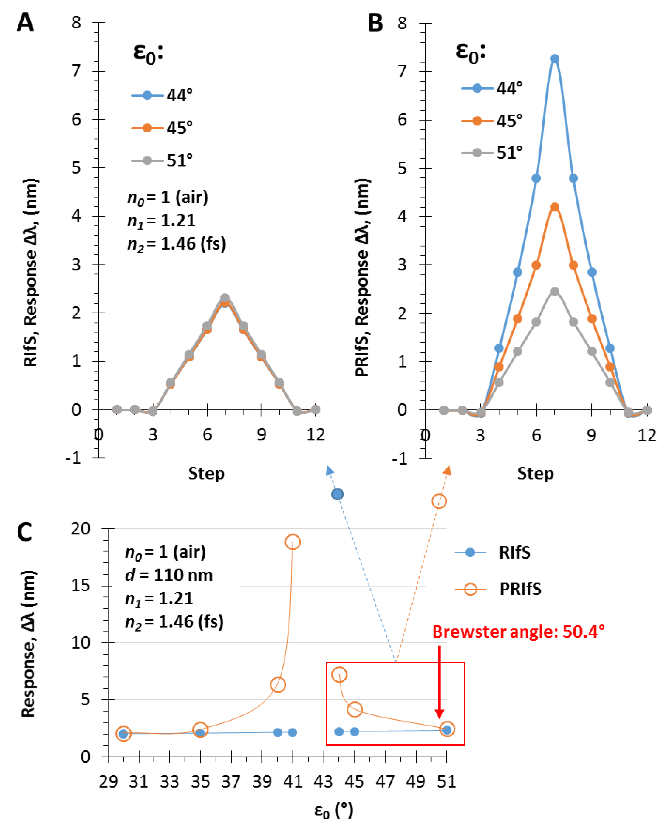
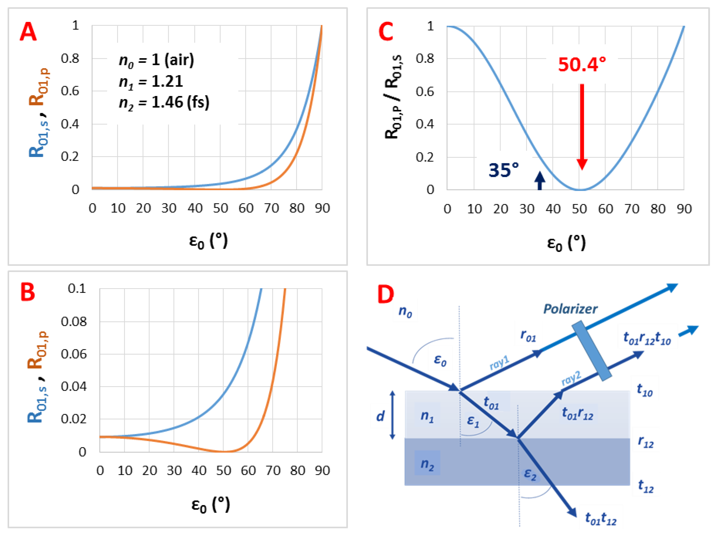
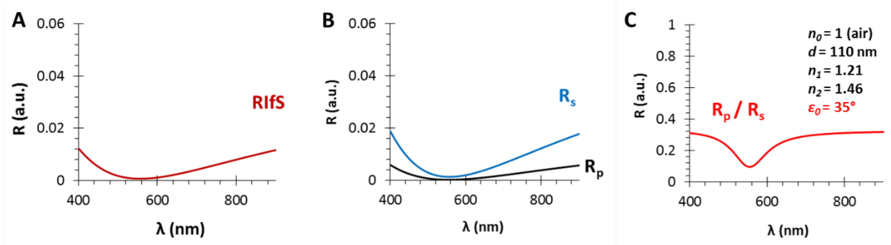
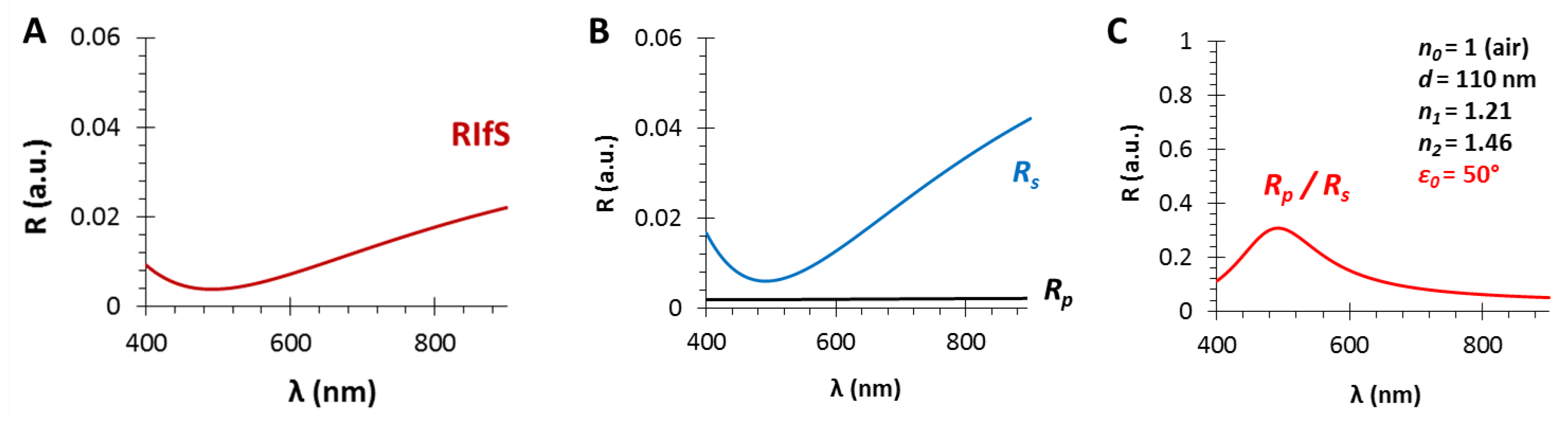
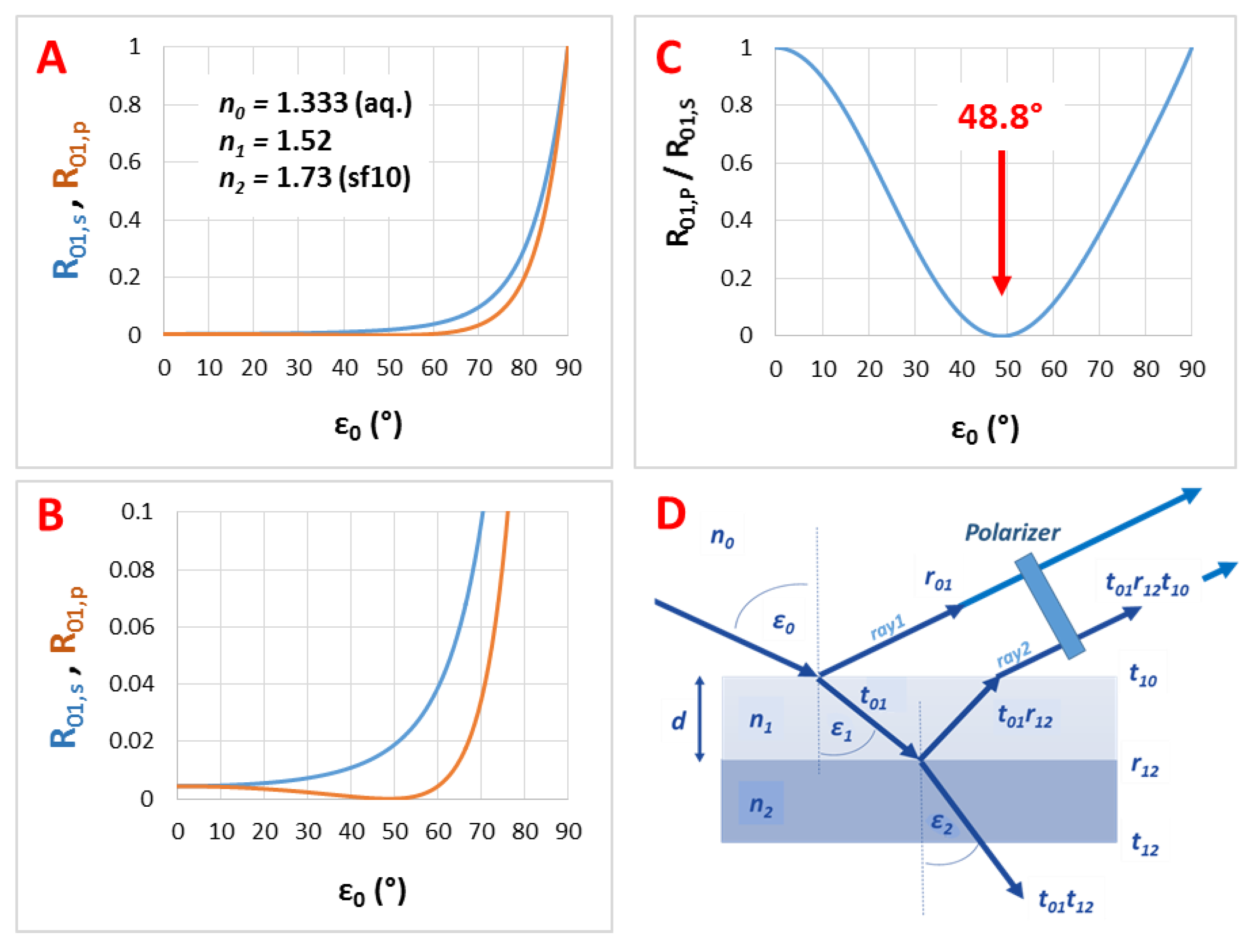
3.3. The Angle of Incidence (ε₀)

In Section 3.1 and Section 3.2, the effect of the thin film thickness and the ratio of the n₀, n₁, n₂ values were investigated. This section focuses on another important (certainly the most important) parameter, namely, the angle of incidence. The selected parameters are n₀ = 1, n₁ = 1.21, n₂ = 1.46 and d = 110 nm, while the angles are ε₀ = 35, 41.5 and 50°. The results are presented in Figure 5. At the interface of the medium and the thin film the Brewster angle is Θ_B = 50.4° with these conditions (see Figure 5A,B and Figure A1), where the parallel component of the reflectance is zero and near this angle the PRIfS curve has a maximum extreme value (Figure 5G,H). By decreasing the incident angle to 35°, where the R_p/R_s ratio is 0.2, the edge shows a red shift, as expected, and the curve has a minimum extreme value (Figure 5C,D). Between these two angles (around ε₀ = 41°), there is a transition region where the contrast of the curve is extremely unfavorable (Figure 5F) and the transition between the minimum and maximum can be observed by zooming (Figure 5F inset). This region is important for two reasons: (1) sensorial applications based on polarized reflectometric interference spectroscopy cannot be carried out in this wavelength range; (2) the optical responses (ΔI and Δλ) of PRIfS technique are 4–7 times higher near this domain, depending on the type of the medium (gas or liquid). Both statements will be verified in the next subsections. These observations and findings are the same in an aqueous medium, with the exception that the Brewster angle is Θ_B,AQ = 48.8°.

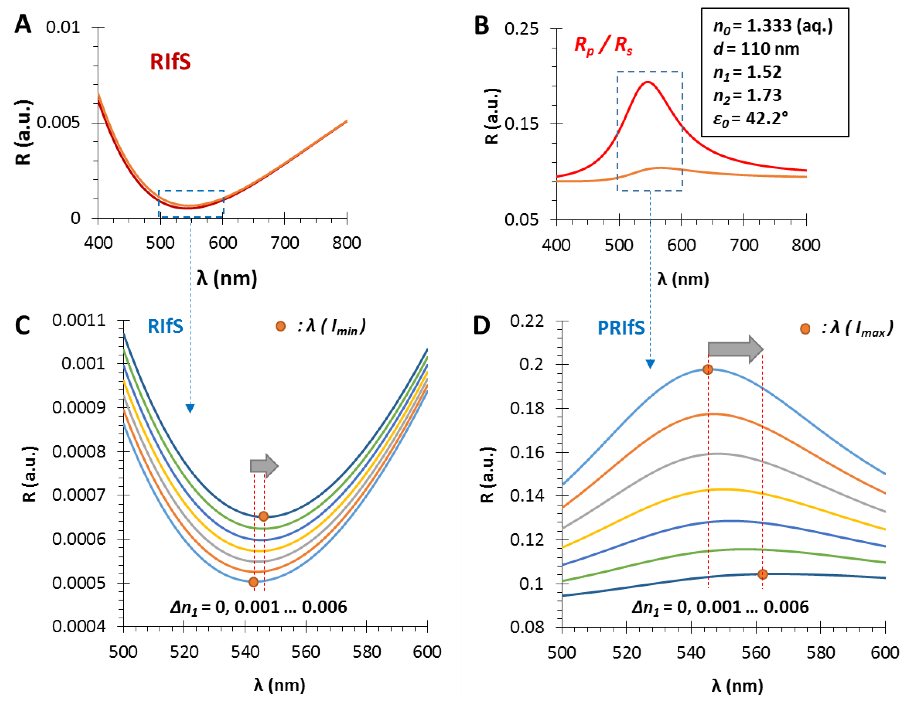
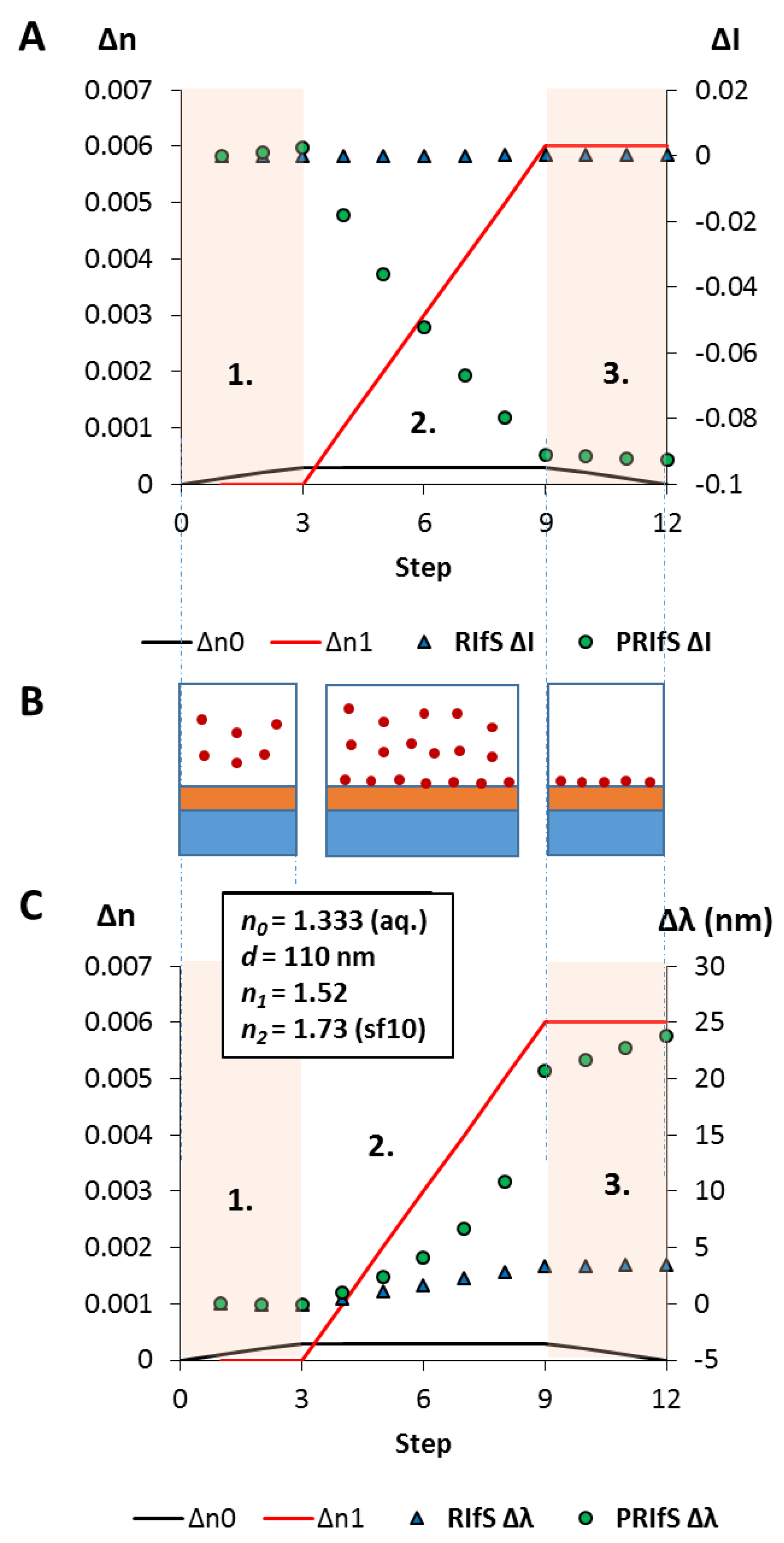
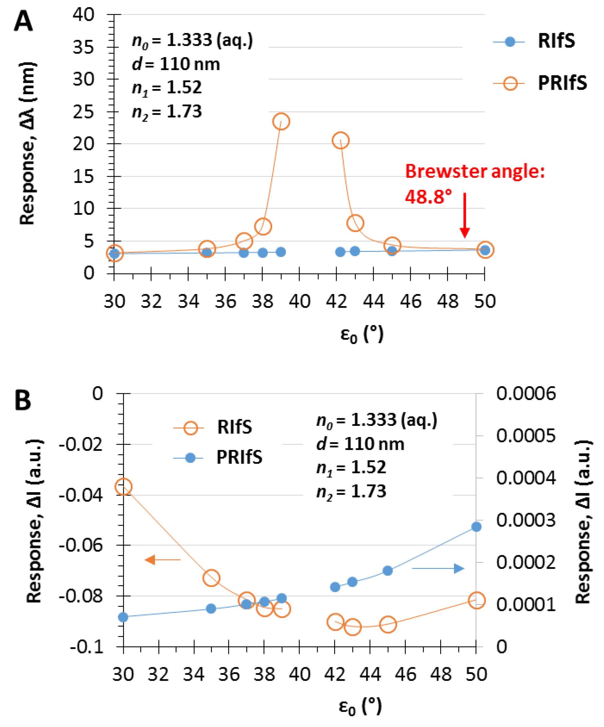
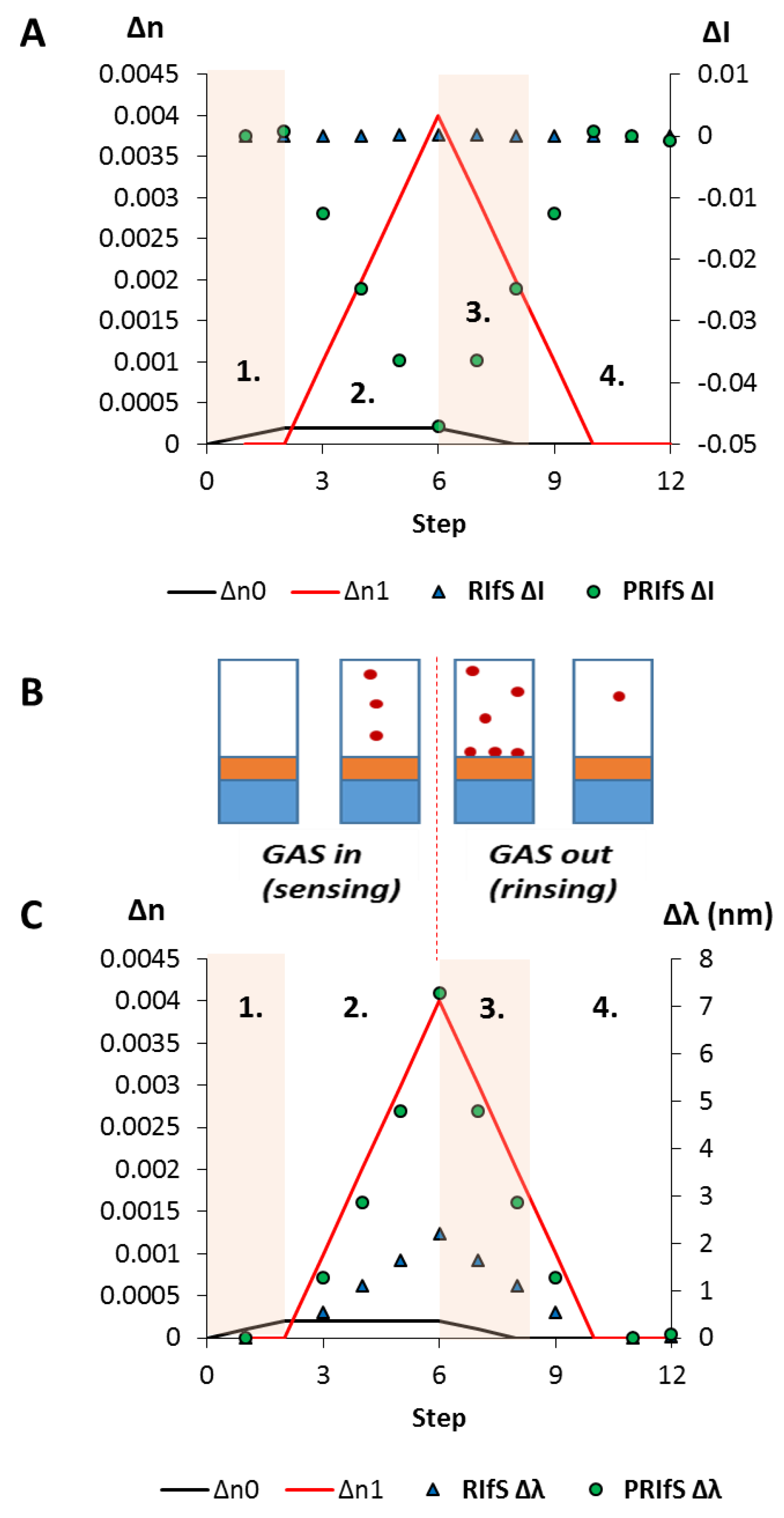
3.4. Simulating an Immobilization Measurement in Aqueous Phase

In Section 3.1, Section 3.2 and Section 3.3, we presented the benefits of using polarized reflected light in reflectometric interference spectroscopy measurements and the optimal conditions were discussed. In this section, a model experiment is presented simulating an adsorption/adhesion/immobilization process. The chosen physical parameters of the model system are the optimal values for the gas phase, as described in Section 3.2 and Section 3.3. Accordingly, the selected parameters are n₀ = 1.333 (aq. medium), d = 110 nm, n₁ = 1.52, n₂ = 1.73 and ε₀ = 42.2° (Figure 6).

In a typical adsorption (immobilization) measurement, and here, during the simulated process, three major steps are examined (see Figure 7B): 1. the dilute solution of the tested molecule reaches the measurement cell, n₀ (near the surface of the sensing layer) is increasing from 1.333 to 1.3333 (Δn₀ = 0.0003); 2. the adsorption/immobilization process occurs, so n₁ increases (from 1.52 to 1.526, Δn₁ = 0.006), indicating the (permanent) presence of the surface excess; 3. the measurement cell is rinsed by pure solvent, n₀ decreases from 1.3333 to 1.333, only the immobilized molecules remain.

The comparison of RIfS and PRIfS curves is presented on Figure 6A–D. As a result of Δn₁ = 0.006, the wavelength shift of the conventional technique is much lower than the Δλ values of the polarized method, as well as the intensity conditions of the latter one being more favorable. However, it can be observed that the contrast of the PRIfS curve is significantly decreased during the process.

Quantitatively: Figure 7A,C shows the ΔI and Δλ curves as the function of the process steps (which can be converted to time in an actual experiment). It can be seen that during the adsorption process, the intensity variations of the conventional and polarized techniques are not on the same scale: ΔI values of PRIfS are higher by two orders of magnitude than RIfS (−0.0921 and 0.00015, respectively). Similar results can be observed in the case of the wavelength shifts: Δλ_RIfS = 3.4 nm, while Δλ_PRIfS = 23.8 nm, which is a seven-fold difference. The calculated sensitivities for RIfS and PRIfS methods are 566 and 3966 nm/RIU (refractive index unit), respectively.

The simulated experiment presented in Figure 7 was carried out by applying an incident angle of ε₀ = 42.2°. Figure 8 shows the ΔI and the Δλ values as the function of ε₀ corresponding to step#9 when Δn₁ = 0.006 and Δn₀ = 0.0003. The similar efficiency of the two methods can be observed at low angle of incidence values and near the Brewster angle (Figure 8A), as well as, the significant improvement of the PRIfS technique near the transition region (see Figure 5F) and the two orders of magnitude difference in ΔI values (Figure 8B). Δλ values in the transition domain are unrealistically high (~100 nm); thus, the simulations cannot be carried out. However, it should be noted that the model experiments are running by assuming ideal attributes, but the real laboratory conditions and the quality of the prepared thin films (such as surface roughness, layer thickness and refractive index inhomogeneity, spot size of the light, etc.) may reduce the ideal nature of the curves. The simulated Δλ sensorgrams corresponding to ε₀ = 42.2, 43 and 45° incident angles (near the transition region) are presented in Figure 9A,B (RIfS and PRIfS, respectively).

3.5. Simulating an Absorption Measurement in Gas Phase

Similar to the simulated immobilization measurement in aqueous phase, a model experiment was carried out by assuming gas phase. The selected parameters were optimal according to Section 3.2 and Section 3.3: n₀ = 1 (air), d = 110 nm, n₁ = 1.21, n₂ = 1.46 and ε₀ = 44°, as presented in Figure 10. Similar to the aqueous medium, the comparison of RIfS and PRIfS curves revealed that the wavelength shift of the conventional technique is much lower than the Δλ values of the polarized method. In addition, it can be observed, that the contrast and the FWHM of the PRIfS curve was not changed significantly during the simulated adsorption process compared to the test carried out in the aqueous phase. The resulting peak values were Δλ_RIfS = 2.2 nm and Δλ_PRIfS = 7.3 nm (see Figure 11C); therefore, the sensitivities were 550 and 1825 nm/RIU for the conventional and the polarized method, respectively, which is almost a four-fold difference. Furthermore, there is a three orders of magnitude difference between the two methods in the ΔI values (see Figure 11A).

The methodology, i.e., the process of the simulation, is slightly different from the immobilization model experiments in the aqueous phase because in this case a reversible adsorption process is studied. The process is demonstrated in Figure 11B, where the steps are: 1. the tested molecules reach the measurement cell by the carrier gas (e.g., N₂) flow, n₀ (near the surface of the sensing layer) increases from 1 to 1.0002 (Δn₀ = 0.0002); 2. the adsorption process occurs, so n₁ increases (from 1.21 to 1.214, Δn₁ = 0.004) because of the reversible physisorbed test molecules; 3. the measurement cell is rinsed by the pure carrier gas, n₀ decreases from 1.0002 to 1; while 4. the weakly physisorbed test molecules leave the surface, and the pores (n₁ decreases from 1.214 to 1.21), finally the original state is restored, and there is no permanent surface excess.

The simulated experiment presented in Figure 10 and Figure 11 was repeated by applying incident angles of ε₀ = 44 and 45°. The results are similar to the aqueous phase experiments: the PRIfS method is significantly more efficient than the conventional technique near the transition domain (see Figure 12A,B), while at low incident angle values and near the Brewster angle, the efficiency of the two methods is comparable (see Figure 12C).

4. Conclusions

In this work, we presented a reflectometric interference sensor applying polarized reflected light. The effect of the refractive indices of the medium, the sensing layer and the substrate, as well as the thin film thickness and the angle of incidence were studied. It was established that the optimal refractive index setting is a crucial condition, namely, the thin films refractive index should be near the geometric mean of the medium and substrate RI. In addition, it was found that the polarization reflectometric interference technique can be used even in the case of films with a layer thickness of d < 150 nm. When examining the effect of the incident angle, we observed that there was a transition region around a critical angle, between the low angles and the Brewster angle, where the contrast of the PRIfS curves considerably decreased, but near this domain the efficiency of the technique significantly increased. Simulated model experiments revealed that the sensitivity of the PRIfS method is nearly four times higher (RIfS: 550 nm/RIU, PRIfS: 1825 nm/RIU) in the gas phase, due to the variation of 0.004 in the sensing layers refractive index, caused by the adsorption/immobilization of test molecules. Similarly, in simulations run in the aqueous phase the difference in was seven-fold: RIfS: 566 nm/RIU, PRIfS: 3966 nm/RIU. Considering these values and assuming a spectral resolution of 10⁻³ nm, a sensitivity of 10⁻⁵–10⁻⁶ RIU can be achieved by the polarization reflectometric interference technique, which is comparable with the sensitivity of the spectroscopic ellipsometry and surface plasmon resonance methods.

References

1. Zhu, Z.; Kao, C.-T.; Wu, R.-J. A highly sensitive ethanol sensor based on Ag@TiO2 nanoparticles at room temperature. Appl. Surf. Sci. 2014, 320, 348–355. [Google Scholar] [CrossRef]
2. Renitta, A.; Vijayalakshmi, K. A novel room temperature ethanol sensor based on catalytic Fe activated porous WO3 microspheres. Catal. Commun. 2016, 73, 58–62. [Google Scholar] [CrossRef]
3. Hazra, A.; Dutta, K.; Bhowmik, B.; Bhattacharyya, P. Repeatable low-ppm ethanol sensing characteristics of p-TiO2-based resistive devices. IEEE Sens. J. 2015, 15, 408–416. [Google Scholar] [CrossRef]
4. Li, X.J.; Chen, S.J.; Feng, C.Y. Characterization of silicon nanoporous pillar array as room-temperature capacitive ethanol gas sensor. Sens. Actuators B Chem. 2007, 123, 461–465. [Google Scholar] [CrossRef]
5. Hosseini, M.S.; Zeinali, S.; Sheikhi, M.H. Fabrication of capacitive sensor based on Cu-BTC (MOF-199) nanoporous film for detection of ethanol and methanol vapors. Sens. Actuators B Chem. 2016, 230, 9–16. [Google Scholar] [CrossRef]
6. Sebők, D.; Janovák, L.; Kovács, D.; Sápi, A.; Dobó, D.G.; Kukovecz, Á.; Kónya, Z.; Dékány, I. Room temperature ethanol sensor with sub-ppm detection limit: Improving the optical response by using mesoporous silica foam. Sens. Actuators B Chem. 2017, 243, 1205–1213. [Google Scholar] [CrossRef] [Green Version]
7. Reichl, D.; Krage, R.; Krummel, C.; Gauglitz, G. Sensing of Volatile Organic Compounds Using a Simplified Reflectometric Interference Spectroscopy Setup. Appl. Spectrosc. 2000, 54, 583–586. [Google Scholar] [CrossRef]
8. Špačková, B.; Wrobel, P.; Bocková, M.; Homola, J. Optical biosensors based on plasmonic nanostructures: A review. Proc. IEEE 2016, 104, 2380–2408. [Google Scholar] [CrossRef]
9. Csapó, E.; Juhász, Á.; Varga, N.; Sebők, D.; Hornok, V.; Janovák, L.; Dékány, I. Thermodynamic and kinetic characterization of pH-dependent interactions between bovine serum albumin and ibuprofen in 2D and 3D systems. Colloids Surf. A 2016, 504, 471–478. [Google Scholar] [CrossRef] [Green Version]
10. Vaisocherová, H.; Víšová, I.; Bocková, M.; Špringer, T.; Ermini, M.L.; Song, X.; Krejčík, Z.; Chrastinová, L.; Pastva, O.; Pimková, K.; et al. Rapid and sensitive detection of multiple MicroRNAs in cell lysate by low-fouling surface plasmon resonance biosensor. Biosens. Bioelectron. 2015, 70, 226–231. [Google Scholar] [CrossRef]
11. Horváth, R.; Pedersen, H.C.; Skivesen, N.; Selmeczi, D.; Larsen, N.B. Optical waveguide sensor for on-line monitoring of bacteria. Opt. Lett. 2003, 28, 1233–1235. [Google Scholar] [CrossRef] [PubMed] [Green Version]
12. Höök, F.; Vörös, J.; Rodahl, M.; Kurrat, R.; Böni, P.; Ramsden, J.J.; Textor, M.; Spencer, N.D.; Tengvall, P.; Gold, J.; et al. A comparative study of protein adsorption on titanium oxide surfaces using in situ ellipsometry, optical waveguide lightmode spectroscopy, and quartz crystal microbalance/dissipation. Colloids Surf. B 2002, 24, 155–170. [Google Scholar] [CrossRef]
13. Sebők, D.; Szendrei, K.; Szabó, T.; Dékány, I. Optical properties of zinc oxide ultrathin hybrid films on silicon wafer prepared by layer-by-layer method. Thin Solid Films 2008, 516, 3009–3014. [Google Scholar] [CrossRef]
14. Pál, E.; Sebők, D.; Hornok, V.; Dékány, I. Structural, optical, and adsorption properties of ZnO2/poly (acrylic acid) hybrid thin porous films prepared by ionic strength controlled layer-by-layer method. J. Colloid Interface Sci. 2009, 332, 173–182. [Google Scholar] [CrossRef]
15. Sebők, D.; Szabó, T.; Dékány, I. Optical properties of zinc peroxide and zinc oxide multilayer nanohybrid films. Appl. Surf. Sci. 2009, 255, 6953–6962. [Google Scholar] [CrossRef]
16. Sebők, D.; Janovák, L.; Dékány, I. Optical, structural and adsorption properties of zinc peroxide/hydrogel nanohybrid films. Appl. Surf. Sci. 2010, 256, 5349–5354. [Google Scholar] [CrossRef]
17. Gauglitz, G.; Krause-Bonte, J.; Schlemmer, H.; Matthes, A. Spectral interference refractometry by diode array spectrometry. Anal. Chem. 1988, 60, 2609–2612. [Google Scholar] [CrossRef]
18. Gauglitz, G.; Brecht, A.; Kraus, G.; Mahm, W. Chemical and biochemical sensors based on interferometry at thin (multi-) layers. Sensor. Actuators B Chem. 1993, 11, 21–27. [Google Scholar] [CrossRef]
19. Sebők, D.; Dékány, I. ZnO2 nanohybrid thin film sensor for the detection of ethanol vapour at room temperature using reflectometric interference spectroscopy. Sensor. Actuators B-Chem. 2015, 206, 435–442. [Google Scholar] [CrossRef]
20. Sebők, D.; Csapó, E.; Ábrahám, N.; Dékány, I. Reflectometric measurement of n-hexane adsorption on ZnO2 nanohybrid film modified by hydrophobic gold nanoparticles. Appl. Surf. Sci. 2015, 333, 48–53. [Google Scholar] [CrossRef]
21. Merkl, S.; Vornicescu, D.; Dassinger, N.; Keusgen, M. Detection of whole cells using reflectometric interference spectroscopy. Phys. Status Solidi. 2014, 211, 1416–1422. [Google Scholar] [CrossRef]
22. Kumeria, T.; Kurkuri, M.D.; Diener, K.R.; Parkinson, L.; Losic, D. Label-free reflectometric interference microchip biosensor based on nanoporous alumina for detection of circulating tumour cells. Biosens. Bioelectron. 2012, 35, 167–173. [Google Scholar] [CrossRef] [PubMed]
23. Piehler, J.; Schreiber, G. Fast transient cytokine-receptor interactions monitored in real time by reflectometric interference spectroscopy. Anal. Biochem. 2001, 289, 173–186. [Google Scholar] [CrossRef] [PubMed]
24. Kasper, M.; Busche, S.; Dieterle, F.; Belge, G.; Gauglitz, G. Quantification of quaternary mixtures of alcohols: A comparison of reflectometric interference spectroscopy and surface plasmon resonance spectroscopy. Meas. Sci. Technol. 2004, 15, 540–548. [Google Scholar] [CrossRef]
25. Hänel, C.; Gauglitz, G. Comparison of reflectometric interference spectroscopy with other instruments for label-free optical detection. Anal. Bioanal. Chem. 2002, 372, 91–100. [Google Scholar] [CrossRef] [PubMed]
26. Pröll, F.; Möhrle, B.; Kumpf, M.; Gauglitz, G. Label-free characterisation of oligonucleotide hybridisation using reflectometric interference spectroscopy. Anal. Bioanal. Chem. 2005, 382, 1889–1894. [Google Scholar] [CrossRef] [PubMed]
27. Zimmermann, R.; Osaki, T.; Gauglitz, G.; Werner, C. Combined microslit electrokinetic measurements and reflectometric interference spectroscopy to study protein adsorption processes. Biointerphases. 2007, 2, 159–164. [Google Scholar] [CrossRef] [Green Version]
28. Leopold, N.; Busche, S.; Gauglitz, G.; Lendl, B. IR absorption and reflectometric interference spectroscopy (RIfS) combined to a new sensing approach for gas analytes absorbed into thin polymer films. Spectrochim. Acta A 2009, 72, 994–999. [Google Scholar] [CrossRef]
29. Kumeria, T.; Losic, D. Controlling interferometric properties of nanoporous anodic aluminium oxide. Nanoscale Res. Lett. 2012, 7, 88. [Google Scholar] [CrossRef]
30. Kumeria, T.; Parkinson, L.; Losic, D. A nanoporous interferometric micro-sensor for biomedical detection of volatile sulphur compounds. Nanoscale Res. Lett. 2011, 6, 634. [Google Scholar] [CrossRef]
31. Choi, H.W.; Takahashi, H.; Ooyaa, T.; Takeuchi, T. Label-free detection of glycoproteins using reflectometric interference spectroscopy-based sensing system with upright episcopic illumination. Anal. Methods UK 2011, 3, 1366–1370. [Google Scholar] [CrossRef]
32. Kurihara, Y.; Takama, M.; Sekiya, T.; Yoshihara, Y.; Ooya, T.; Takeuchi, T. Fabrication of Carboxylated Silicon Nitride Sensor Chips for Detection of Antigen–Antibody Reaction Using Microfluidic Reflectometric Interference Spectroscopy. Langmuir 2012, 28, 13609–13615. [Google Scholar] [CrossRef] [PubMed]
33. Choi, H.W.; Sakata, Y.; Kurihara, Y.; Ooya, T.; Takeuchi, T. Label-free detection of C-reactive protein using reflectometric interference spectroscopy-based sensing system. Anal. Chim. Acta 2012, 728, 64–68. [Google Scholar] [CrossRef] [PubMed]
34. Heavens, O.S. Thin Film Physics, 1st ed.; Methuen: London, UK, 1972; pp. 62–66. [Google Scholar]
35. Refractive Index of Fused Silica—Malitson. 1965. Available online: https://refractiveindex.info/?shelf=glass&book=fused_silica&page=Malitson (accessed on 11 May 2019).
36. Refractive Index of SF10—SCHOTT. Available online: https://refractiveindex.info/?shelf=glass&book=SF10&page=SCHOTT (accessed on 11 May 2019).
Figure 1. The schematic diagram of a typical reflectometric interference setup and thin film model for the calculations: n, ε, r and t mark refractive index, refraction angle, reflection and transmission amplitudes (calculated by Fresnel equations), and the indices 0, 1 and 2 represent medium, thin film and substrate, respectively. The curves show the spectrum of the light source and the measured reflectance (which is defined here as the ratio of the s- and p-polarized component).
Photonics 06 00076 g001
Figure 2. The calculated reflectance curves from a thin film with a thickness d = 800 nm and an effective refractive index n1 = 1.38 (using SF10 substrate with n2 = 1.7, in air, ε0 = 35°): (A) The conventional reflectance (RIfS) curve with the interference pattern, calculated by Equation (7); (B) The s- and p-polarized components of (A) and their average, calculated by Equations (12) and (13); (C) The polarized reflectance curve, which can be measured as the ratio of s- and p-polarized components, calculated by Equation (14).
Photonics 06 00076 g002
Figure 3. The calculated reflectance curves from thin films with an effective refractive index of n1 = 1.21 and different film thicknesses (A,B), (C,D) and (E,F), d = 110, 135 and 160 nm, respectively (using fused silica substrate with n2 = 1.46, in air, ε0 = 30°): (A,C,E) The s- and p-polarized components of the conventional RIfS curves (Equations (12) and (13)) and the zoom in the region where RS and RP curves get closer; (B,D,F) the ratio of the s- and p-polarized components (Equation (14)).
Photonics 06 00076 g003
Figure 4. The calculated polarized reflectance curves from thin films with a film thickness of d = 110 nm and different effective refractive indices (using fused silica substrate with n2 = 1.46, in air, ε0 = 35°): (A,C,E) The s- and p-polarized components of the conventional RIfS curves (from Equations (12) and (13)); and (B,D,F) The ratio of the s- and p-polarized components (from Equation (14)) in the case of n1 = 1.21, 1.32 and 1.52 thin film refractive indices, respectively; n1 values are optimized and calculated as the geometric mean of n0 and n2.
Photonics 06 00076 g004
Figure 5. (A) The calculated (s- and p-polarized) reflectance curves and (B) their ratio as the function of the incident angle (ε0) for a gas/thin film interface with n0 = 1 and n1 = 1.21; (C,E,G): The calculated (s- and p-polarized) reflectometric interference curves and (D,F,H) their ratios in the case of an n1 = 1.21 and d = 110 nm thin film on fused silica substrate (n2 = 1.46), in air, with different incident angles, ε0 = 35, 41.5 and 50°, respectively.
Photonics 06 00076 g005
Figure 6. The calculated reflectometric interference curves for (A) the conventional and (B) the polarization method, in the case of an n1 = 1.52 and d = 110 nm thin film on SF10 substrate (n2 = 1.73), in aqueous medium, by applying an incident angle of ε0 = 42.2°; during the measurement ΔR and Δλ values are monitored as the function of Δn1; (C,D) The region of interest zooms to the red shift of the RIfS and PRIfS curves, while n1 increases from 1.52 to 1.526.
Photonics 06 00076 g006
Figure 7. The results of the simulated model experiment: (A) The ΔI curves for the conventional (RIfS ΔI) and the polarized (PRIfS ΔI) cases due to Δn0 = ± 0.0003 (steps 1. and 3.) or Δn1 = 0.006 (adsorption, step 2.); (B) Schematic drawings of the steps: 1. the dilute solution of the analyte reaches the measurement cell, 2. the immobilization process, 3. rinsing of the measurement cell; (C) The Δλ curves for the conventional (RIfS Δλ) and the polarized (PRIfS Δλ) cases due to Δn0 = ± 0.0003 (ranges 1. and 3.) or Δn1 = 0.006 (adsorption, range 2.).
Photonics 06 00076 g007
Figure 8. Maximal (A) Δλ and (B) ΔI responses of RIfS (yellow) and PRIfS (blue) techniques due to Δn0 = 0.0003 and Δn1 = 0.006 refractive index changes as the function of the incident angle ε0, in the case of a thin film with d = 110 nm and n1 = 1.52 on SF10 substrate, in aqueous medium.
Photonics 06 00076 g008
Figure 9. Δλ sensorgrams of (A) RIfS and (B) PRIfS techniques at different incident angles (ε0 = 42.2, 43 and 45°), due to Δn0 = ± 0.0003 (steps #1–3 and #10–12) and Δn1 = 0.006 (steps #4–9) refractive index changes, in the case of a thin film with d = 110 nm and n1 = 1.52 on SF10 substrate, in aqueous medium.
Photonics 06 00076 g009
Figure 10. The calculated reflectometric interference curves for (A) the conventional and (B) the polarization method, in the case of an n1 = 1.21 and d = 110 nm thin film on fused silica substrate (n2 = 1.46), in air, by applying an incident angle of ε0 = 44°; during the measurement, ΔR and Δλ values are monitored as a function of Δn1; (C,D) The region of interest zooms to the red shift of the RIfS and PRIfS curves, while n1 increases from 1.21 to 1.214.
Photonics 06 00076 g010
Figure 11. The results of the simulated model experiment: (A) The ΔI curves for the conventional (RIfS ΔI) and the polarized (PRIfS ΔI) cases due to Δn0 = ±0.0002 (steps 1. and 3.) or Δn1 = ±0.004 (adsorption, step 2.; desorption, step 4.); (B) Schematic drawing of the steps: 1. the tested molecules reach the measurement cell by the carrier gas (e.g., N2) flow; 2. the adsorption process occurs; 3. the measurement cell is rinsed by the pure carrier gas; while 4. the weakly physisorbed test molecules leave the surface and the pores; (C) The Δλ curves for the conventional (RIfS Δλ) and the polarized (PRIfS Δλ) cases due to Δn0 = ±0.0002 (ranges 1. and 3.) or Δn1 = ±0.004 (adsorption, range 2.; desorption, range 4.).
Photonics 06 00076 g011
Figure 12. Δλ sensorgrams of (A) RIfS and (B) PRIfS techniques at different incident angles (ε0 = 44, 45 and 51°), due to Δn1 = ±0.004 refractive index changes (steps #4–9), in the case of a thin film with d = 110 nm and n1 = 1.21 on fused silica substrate, in air; (C) Maximal Δλ responses of RIfS (yellow) and PRIfS (blue) techniques due to Δn0 = 0.0002 and Δn1 = 0.004 refractive index changes as the function of the incident angle ε0.
Photonics 06 00076 g012